Large Eddy Simulation Study of H2/CH4 Flame Structure at MILD ...
Large Eddy Simulation Study of H2/CH4 Flame Structure at MILD ...
Large Eddy Simulation Study of H2/CH4 Flame Structure at MILD ...

You also want an ePaper? Increase the reach of your titles
YUMPU automatically turns print PDFs into web optimized ePapers that Google loves.
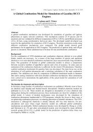
MCS 7 Chia Laguna, Cagliari, Sardinia, Italy, September 11-15, 2011<br />
<strong>Large</strong> <strong>Eddy</strong> <strong>Simul<strong>at</strong>ion</strong> <strong>Study</strong> <strong>of</strong> <strong>H2</strong>/<strong>CH4</strong> <strong>Flame</strong> <strong>Structure</strong> <strong>at</strong><br />
<strong>MILD</strong> Condition<br />
Y. Afarin*, S. Tabejama<strong>at</strong>* and A. Mardani *<br />
Yashar-afarin@aut.ac.ir<br />
*Department <strong>of</strong> Aerospace Engineering, Amirkabir University <strong>of</strong> Technology, Tehran, Iran<br />
Abstract<br />
This paper demonstr<strong>at</strong>es the large eddy simul<strong>at</strong>ion (LES) <strong>of</strong> a <strong>H2</strong>/<strong>CH4</strong> jet in a hot and diluted<br />
co-flow stream which emul<strong>at</strong>ed the <strong>MILD</strong> combustion regime. The turbulence-combustion<br />
interaction is modeled using the CPaSR model while the reduced chemical mechanism <strong>of</strong><br />
DRM-22 represents the chemical reactions. <strong>Structure</strong> <strong>of</strong> <strong>MILD</strong> combustion regime for two<br />
co-flow oxygen concentr<strong>at</strong>ion <strong>of</strong> 3 and 9% (by mass) are investig<strong>at</strong>ed. The reaction zone<br />
structure is shown by the temper<strong>at</strong>ure distribution and distribution <strong>of</strong> OH, CH 2 O and HCO<br />
mass fraction. Results show th<strong>at</strong> the measurements are predicted with an acceptable accuracy.<br />
Moreover, the extinction and re-ignition phenomena th<strong>at</strong> take place under this combustion<br />
regime is captured by the current numerical method. The l<strong>at</strong>er phenomena occur in a larger<br />
zone by decreasing the O 2 concentr<strong>at</strong>ion as well as the reaction zone expands.<br />
Introduction<br />
Rapid industrial development during recent decades in addition to problems rel<strong>at</strong>ed to global<br />
warming and reduction in fossil energy resources criticized the current situ<strong>at</strong>ion. In this<br />
circumstances utilizing new technology seems to be critically necessary in order to decrease<br />
pollutions and increase the combustion efficiency. <strong>MILD</strong> (Moder<strong>at</strong>e or Intense Low-oxygen<br />
Dilution) combustion [1] is a promising candid<strong>at</strong>e for replacing the old combustion<br />
technology due to its specific characteristics consist <strong>of</strong> increasing thermal efficiency and<br />
decreasing the pollution emission. This technology has been successfully applied in several<br />
industries [2] but doing more studies are necessary to investig<strong>at</strong>e its combustion<br />
characteristics [1,3].<br />
To emul<strong>at</strong>e <strong>MILD</strong> combustion regime, Dally et al. [3] designed and used a burner in which a<br />
jet <strong>of</strong> fuel (CH 4 / H 2 ) is injected in hot c<strong>of</strong>low oxidant stream. In their research influence <strong>of</strong><br />
different O 2 mass fraction c<strong>of</strong>low on flame structure <strong>at</strong> different loc<strong>at</strong>ion from the nozzle were<br />
studied. Their experimental results were used by some other researchers as a reference to<br />
assess their numerical results. Among them, Christo et al. [4] compared various turbulence<br />
chemistry interaction models and also qualified the k-ε model in <strong>MILD</strong> combustion. They<br />
also reported th<strong>at</strong>, <strong>MILD</strong> combustion modeling is beyond the capability <strong>of</strong> single conserved<br />
scalar-based models. Frassold<strong>at</strong>i et al. [5] studied different modeling approaches on flame<br />
structure prediction in <strong>MILD</strong> combustion by using FLUENT. According to their result the<br />
accuracy <strong>of</strong> the numerical solution, especially for the turbulent intensity, is sensitive to the<br />
boundary conditions. Mardani et al. [6] clarify the importance <strong>of</strong> differential diffusion method<br />
on flame structure under <strong>MILD</strong> combustion conditions. They showed th<strong>at</strong> the molecular<br />
transport<strong>at</strong>ion has a strong effect on flame structure. LES modeling <strong>of</strong> <strong>MILD</strong> combustion<br />
regime was performed by Ihme et al. [7] where they used a presumed probability density
function to model the turbulent chemistry interaction on unresolved scales. They discussed<br />
the importance <strong>of</strong> vari<strong>at</strong>ions in scalar inflow conditions on turbulent combustion under <strong>MILD</strong><br />
combustion regime. They found th<strong>at</strong> LES modeling has the capability to be used in this<br />
regime but boundary conditions could have a significant effect on the final results.<br />
Kobayashi et al. [8] experimentally investig<strong>at</strong>e the flame structure under high temper<strong>at</strong>ure air<br />
combustion. They found th<strong>at</strong> flow turbulence have a pr<strong>of</strong>ound effect in decreasing NOx<br />
emission. Also, according to their result the turbulence is the main factor <strong>of</strong> OH suppressions<br />
and local flame extinctions. In this regard, Medwell et al. [9] investig<strong>at</strong>ed the effect <strong>of</strong> fuel<br />
Reynolds number on <strong>MILD</strong> flame structure. According to their results, increasing the<br />
Reynolds number intensifies the convolution and weakening the OH distribution. Obviously<br />
from the above researches, turbulence has the important effect on local flame suppression.<br />
In the <strong>MILD</strong> combustion regime, the mean flow velocity is high to provide a combustible<br />
mixture with low oxygen level and which also prevents the hot spots in combustion chamber.<br />
It is necessary to have both extinction and re-ignition, especially near the nozzle exit zone, in<br />
order to have the <strong>MILD</strong> combustion condition. Such local extinction and re-ignition are<br />
investig<strong>at</strong>ed experimentally by Kobayashi et al. [8]. Numerical investig<strong>at</strong>ions <strong>of</strong> the <strong>MILD</strong><br />
combustion by Christo et al. [4] and Mardani et al. [6] are indic<strong>at</strong>ed th<strong>at</strong> although the effect<br />
<strong>of</strong> turbulence on controlling the flame is important, the influence <strong>of</strong> finite r<strong>at</strong>e chemistry<br />
never can be negligible in <strong>MILD</strong> regime. Based on the above mentioned researches,<br />
turbulence chemistry interaction has a pr<strong>of</strong>ound effect on the numerical results <strong>at</strong> <strong>MILD</strong><br />
combustion.<br />
Many investig<strong>at</strong>ions have been performed to study turbulent chemistry modeling <strong>at</strong> <strong>MILD</strong><br />
combustion. Among them, the <strong>Eddy</strong> Dissip<strong>at</strong>ion Concept [10], EDC, model has the possibility<br />
to couple CFD simul<strong>at</strong>ion and detailed kinetic more simply than other models. Therefore<br />
there was a gre<strong>at</strong> interest to use this model specially when the comput<strong>at</strong>ional cost is high.<br />
Christo et al. [4], Mardani et al. [6] and Frassold<strong>at</strong>i et al. [5] used EDC and reported the<br />
reasonably accur<strong>at</strong>e results compared with experimental measurements. In all <strong>of</strong> these<br />
researches model were used as the turbulence model.<br />
In the current research, flame structure under <strong>MILD</strong> combustion regime is investig<strong>at</strong>ed. For<br />
the first time, combin<strong>at</strong>ion <strong>of</strong> large eddy simul<strong>at</strong>ion to model turbulence quantity and a<br />
modified version <strong>of</strong> EDC referenced by Chalmers Partially Stirred Reactor Model (CPaSR),<br />
Chomiak and Karlsson [11], is considered to calcul<strong>at</strong>e the turbulence-chemistry interactions.<br />
This study focuses on experimental measurements <strong>of</strong> Dally et al. [3]. The purpose <strong>of</strong> this<br />
study is discussing about local flame extinction under <strong>MILD</strong> combustion regime.<br />
Numerical Method and Governing Equ<strong>at</strong>ions<br />
In this paper, compressible Navier-Stokes equ<strong>at</strong>ions (NSE) is used to describe the flow. In<br />
<strong>Large</strong> <strong>Eddy</strong> <strong>Simul<strong>at</strong>ion</strong>, filtering the dependent variables divide them into GS and SGS<br />
components in a way th<strong>at</strong> , where is resolved part. In this study, box filter<br />
is used to filter variables, where refers to grid size in direction.<br />
According to Favre approach a filtering oper<strong>at</strong>ion is weighted by the density according to<br />
following the equ<strong>at</strong>ion:<br />
( 1 )<br />
By filtering the variables in compressible NSE and using the Smagoronisky model [12], the<br />
instantaneous balance filtered equ<strong>at</strong>ions leads to the following equ<strong>at</strong>ions. These equ<strong>at</strong>ions<br />
formally are similar to Reynolds averaged balance equ<strong>at</strong>ions [13]:
4<br />
4 4 7 45 6 / ( 2 )<br />
<br />
><br />
4 8 "<br />
4 97 4 45 6 8 " : 4 ;( ( )*)<br />
4 8 "<br />
< = <br />
45 #$ % 45 "<br />
<br />
.? @ ? A ( 3)<br />
47<br />
6<br />
4 4 97 45 6 7 B : 4 4 ;C 45 45 6B ( )*) ; 4 76<br />
4 76<br />
< E D<br />
45 D 45 F ! ""< (4)<br />
4<br />
4 4 97 45 6 : G <br />
G 4 ; ( 45 &' ( )*)<br />
4 <br />
<<br />
&' % 45 <br />
(5)<br />
where is the velocity vector, is the pressure, is the flow density, is the enthalpy and <br />
is the mass fraction <strong>of</strong> species. The isotropic contribution, ! "" , in equ<strong>at</strong>ion (which is twice<br />
the subgrid scale turbulent kinetic energy) is unknown and usually absorbed into the filtered<br />
pressure [13]. In the above equ<strong>at</strong>ions #$ % and &' % are considered as unity. All terms in above<br />
equ<strong>at</strong>ions are closed except the species transport’s (Eq. 3) source term. The ( )*) is the subgrid<br />
scale viscosity which is computed according to the below mentioned equ<strong>at</strong>ion:<br />
H )*) + " I (6 )<br />
where + " is set to 0.02 in this study. The term , )*) is defined as:<br />
, )*) + -I<br />
(7 )<br />
where + - is constant and set to 1.048.<br />
In the present study, the OpenFOAM (Open Field Oper<strong>at</strong>ion and Manipul<strong>at</strong>ion) CFD<br />
toolbox is used to solve transport equ<strong>at</strong>ions. OpenFOAM is a package <strong>of</strong> free and open source<br />
object oriented C++ codes, Weller et.al [14]. The PISO ( Pressure Implicit with Splitting <strong>of</strong><br />
Oper<strong>at</strong>ors) method [15] is used to solve NSE in an unsteady configur<strong>at</strong>ion. Its preference is<br />
due to two factors. This method needs no under-relax<strong>at</strong>ion and the momentum corrector step<br />
is recalled more than one time. Briefly this solver is based on unsteady PISO with two<br />
pressure correctors and two momentum correctors with time step ./ 01 2 and convergence<br />
criteria for residuals ./ 3.. . For more inform<strong>at</strong>ion about how OpenFOAM uses this procedure,<br />
one may refer to Ref. [16]. The implicit first order bounded Euler scheme is used to discrete<br />
the unsteady term. The convection and diffusion terms are discretized using the Normalized<br />
Variable Diagram (NVD) Scheme and the second order central difference schemes,<br />
respectively. Mass flux calcul<strong>at</strong>ion is done by Linear (second order central difference)<br />
interpol<strong>at</strong>ion.<br />
In the present study, modified version <strong>of</strong> the reactingFoam (change from RANS to LES)<br />
th<strong>at</strong> is one <strong>of</strong> the reacting flow solvers <strong>of</strong> OpenFOAM is used. This solver uses the CPaSR as<br />
a turbulent chemistry interaction model. Indeed, the basic difference between EDC and<br />
CPaSR is in computing approach <strong>of</strong> the chemical timescale. In CPaSR model, the flame<br />
thickness is assumed to be much thinner than usual comput<strong>at</strong>ional cell, therefore cell space<br />
should be split into two parts; reacting part and non-reacting part. The theory postul<strong>at</strong>e th<strong>at</strong> in<br />
reacting part, like a perfectly stirred reactor, all species are perfectly stirred and react during<br />
reaction time. After reactions takes place, the species (burned and unburned) are assumed to
e mixed due to turbulence during mixing time, C J , and then final concentr<strong>at</strong>ion is<br />
composed <strong>of</strong> burned and unburned species. The important inform<strong>at</strong>ion lies in defining mixing<br />
time, C J , chemical time scale, C K , and description <strong>of</strong> each comput<strong>at</strong>ional cell division<br />
process. The chemical time scale,C K , is determined by solving the reaction system's fully<br />
coupled ODEs, and finding the characteristic time for th<strong>at</strong> system. The turbulence mixing<br />
time is rel<strong>at</strong>ed to effective viscosity, mean density, and sub-grid scale turbulent dissip<strong>at</strong>ion<br />
according to the below equ<strong>at</strong>ion:<br />
C J + J V ( ( )*)<br />
, )*)<br />
( 8 )<br />
where + J .. In all above expressions is SGS kinetic energy.<br />
R<strong>at</strong>e <strong>of</strong> reaction for specie L can be scaled by reactive volume fraction M, as:<br />
4+ <br />
4 + <br />
+ W<br />
C<br />
O XX + (9)<br />
where C is the residence time (numerical time step), + N is defined as initial concentr<strong>at</strong>ion <strong>of</strong><br />
species in a control volume, + is final concentr<strong>at</strong>ion <strong>of</strong> species in a control volume, and M<br />
(kappa) which takes a value between 0 to 1 is defined as:<br />
O <br />
C K C<br />
C K C J C<br />
(10)<br />
One <strong>of</strong> the most important parameter in current study th<strong>at</strong> can be used to clarify the<br />
turbulent and chemistry interaction is O. This factor changes the species transport equ<strong>at</strong>ion as<br />
below:<br />
4 <br />
4 Y Z Y9( -[[ Y : # OXX + (11)<br />
Based on its definition, the value <strong>of</strong> this term is one, for a control volume without any<br />
reactions or where the chemical timescale is much larger than the mixing time scale,<br />
(P Q RP SLT ). But in situ<strong>at</strong>ions th<strong>at</strong> the process <strong>of</strong> mixing and reaction have the same time scale<br />
orders, this term has the value lower than one. Thus briefly, by increasing the turbulence<br />
intensity and thereby decreasing the C J in reaction zone, O approaches to unity.<br />
It should be noted th<strong>at</strong> this model is different from the stochastic one which is based on a<br />
simplified joint composition probability density function transport equ<strong>at</strong>ion and is known as<br />
PaSR model.<br />
The 3D comput<strong>at</strong>ional domain is constructed according to the experimental burner<br />
geometry <strong>of</strong> Dally et al. [3]. It is a H 2 /CH 4 jet in Hot Co-flow (JHC) mounted in a wind tunnel<br />
with an air flows <strong>of</strong> 3.2 m Us<br />
parallel to the burner axis. The JHC burner consists <strong>of</strong> a fuel and<br />
a hot c<strong>of</strong>low jet which are mounted in a wind tunnel with air flows ( 23% O 2 +77% N 2 (mass<br />
basis )). Fig. 1 shows different sections <strong>of</strong> the Dally et.al [3] burner, schem<strong>at</strong>ically.<br />
Inlet boundary conditions, for mean species mass fractions and mean velocity pr<strong>of</strong>iles, are<br />
set using the results <strong>of</strong> a separ<strong>at</strong>e modeling <strong>at</strong> upstream <strong>of</strong> burner exit plane. The mean inlet<br />
velocity <strong>of</strong> hot co-flow mixture and wind tunnel air are 3.2 m/s and the mean inlet velocity <strong>of</strong>
fuel jet is around 100 m/s. The inlet temper<strong>at</strong>ure <strong>of</strong> fuel mixture, hot co-flow mixture and air<br />
are 305, 1300 and 300 K, respectively. The inlet Reynolds number <strong>of</strong> fuel mixture on the<br />
basis <strong>of</strong> fuel mixture jet velocity and temper<strong>at</strong>ure is approxim<strong>at</strong>ely equal to 10000. Mardani et<br />
al. [6 ], Christo et al. [4] and Frassold<strong>at</strong>i et al. [5] reported th<strong>at</strong> the results are not sensible to<br />
turbulence intensity <strong>at</strong> the hot co-flow and wind tunnel, but the value <strong>of</strong> turbulent intensity <strong>of</strong><br />
the fuel inlet has very significant effect on numerical results. Because the value <strong>of</strong> turbulent<br />
intensity <strong>of</strong> fuel inlet was not indic<strong>at</strong>ed by Dally et al. [3], different researchers used different<br />
values <strong>of</strong> fuel inlet turbulent intensity. For instance, although the experimentally measured<br />
turbulent kinetic energy is reported as 16 m 2 /s 2 <strong>at</strong> the fuel inlet by Christo et al. [4], they<br />
preferred to use mean turbulent kinetic energy <strong>of</strong> 60 m 2 /s 2 (7.5% turbulent intensity). Also,<br />
Mardani et al. [6] adjusted it to 7% in order to have a better agreement between the numerical<br />
and experimental results. In the present research, the turbulence intensity <strong>at</strong> the fuel inlet is set<br />
to 7%.<br />
Figure 1. Schem<strong>at</strong>ic <strong>of</strong> Dally et al. [3] burner<br />
A grid study with a number <strong>of</strong> control volumes approxim<strong>at</strong>ely between 8\ ./ ] to<br />
1.1\ ./ 1 is performed and finally an unstructured grid with about 9×./ ] cells is selected.<br />
Detailed inform<strong>at</strong>ion about the cases are shown in Table 1. These cases are considered to<br />
study the effect <strong>of</strong> turbulence on flame structure on the <strong>MILD</strong> combustion characteristics <strong>of</strong><br />
methane-hydrogen mixture <strong>at</strong> different co-flow oxygen content.<br />
The DRM-22 chemical mechanism, [17], is considered for modeling <strong>of</strong> combustion<br />
reactions. It is a reduced mechanism <strong>of</strong> GRI 1.2 [18] with 22 species, including Ar and N2,<br />
for a total 104 reversible reactions. The results <strong>of</strong> Mardani et al.[6] show the good<br />
performance <strong>of</strong> the DRM-22 for comput<strong>at</strong>ion chemical reactions under <strong>MILD</strong> combustion<br />
conditions.<br />
Table 1. Specific<strong>at</strong>ions <strong>of</strong> numerical study<br />
Case Fuel Composition Hot Oxidizer Composition Chemical Mechanism<br />
1 20%H 2 +80%CH 4 9%O 2 +6.5%H 2 O+5.5%CO 2 +79%N 2 DRM-22 [17]<br />
2 20%H 2 +80%CH 4 3%O 2 +6.5%H 2 O+5.5%CO 2 +85%N 2 DRM-22 [17]<br />
Numerical Results<br />
Before any results discussion it is necessary to assess the quality <strong>of</strong> the LES method th<strong>at</strong> is<br />
used in the present research. Klein [19] studied a method to evalu<strong>at</strong>e large eddy simul<strong>at</strong>ion in<br />
the context <strong>of</strong> Implicit filtering. He declared th<strong>at</strong> computing the numerical error in LES
method is more complic<strong>at</strong>ed in comparison with RANS. In LES method, the error is caused<br />
by two overlapping factors; subgrid parameteriz<strong>at</strong>ion and numerical contamin<strong>at</strong>ion <strong>of</strong> the<br />
smaller retained structure [19]. Pope [20] demonstr<strong>at</strong>ed th<strong>at</strong> a good LES should resolve <strong>at</strong><br />
least 80% <strong>of</strong> the TKE. A new parameter was defined by [20] to present r<strong>at</strong>io <strong>of</strong> resolved to<br />
total kinetic energy:<br />
'a2bcdae !fg 'h b <br />
i-jWkl-m<br />
i-jWkl-m )*)<br />
( 12 )<br />
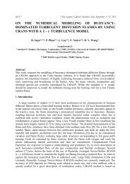
Fig. 2 illustr<strong>at</strong>es resolved TKE r<strong>at</strong>io for flame with different percent <strong>of</strong> oxygen in<br />
different distances from the nozzle exit. As can be seen, in all cases, more than 94 % <strong>of</strong> total<br />
TKE was resolved directly and according to Ref. [20], results from the LES modeling with<br />
this characteristics could be reliable.<br />
Figure 2. Resolved turbulent kinetic energy r<strong>at</strong>ion in case 1 and 2 in Table 1, on a line <strong>at</strong> 30<br />
mm and 60 mm from the nozzle exit.<br />
Dally’s measurements [3], are used for valid<strong>at</strong>ion <strong>of</strong> the results <strong>of</strong> the present study . Figs<br />
.3 and 4 shows distribution <strong>of</strong> CO, OH, CO 2 mass fraction and temper<strong>at</strong>ure versus mean<br />
mixture fraction <strong>at</strong> two distances, 30 mm and 60 mm, from the nozzle exit and for two, 3%<br />
and 9%. percent <strong>of</strong> oxygen in co-flow. Mean mixture fraction (^, is calcul<strong>at</strong>ed using the<br />
Bilger’s [21] expression:<br />
n ; o9_ p _ p?q :<br />
`p<br />
o_ p?s _ p?q <br />
`p<br />
9_ r _ r?q :<br />
o`r<br />
_ r?s _ r?q <br />
o`r<br />
9_ q _ q?q :<br />
<<br />
`q<br />
_ q?s _ q?q <br />
<br />
`q<br />
(13)<br />
In the above equ<strong>at</strong>ion, _ represent the value <strong>of</strong> conserved scalar th<strong>at</strong> is given by mass<br />
fraction <strong>of</strong> element and ` is referred to the <strong>at</strong>omic mass <strong>of</strong> element . Detailed inform<strong>at</strong>ion<br />
about computing _ is resented <strong>at</strong> [21]. Also, according to Christo and Dally [4], the effect <strong>of</strong><br />
thermal radi<strong>at</strong>ion on numerical results is considered negligible.
As can be seen from Figs. 3 and 4, the numerical and experimental results are in good<br />
agreement. Some differences in Figs. 3 and 4 could be referred to acceptable accuracy <strong>of</strong><br />
chemical reaction calcul<strong>at</strong>ions and flow dynamic modeling or may be experimental accuracy.<br />
CO2 Mass Fraction<br />
0 0.05 0.1 0.15<br />
Temper<strong>at</strong>ure (k)<br />
300 600 900 1200 1500 1800 2100<br />
Numeric , Z=30mm<br />
EXP, Temper<strong>at</strong>ure<br />
EXP, CO<br />
EXP, CO2<br />
EXP, OH<br />
0.2 0.4 0.6<br />
Mixture Fraction<br />
CO Mass Fraction<br />
0 0.02 0.04 0.06 0.08<br />
0 0.002 0.004 0.006 0.008 0.01 0.012 0.014<br />
OH Mass Fraction<br />
CO2 Mass Fraction<br />
0 0.05 0.1 0.15<br />
Temper<strong>at</strong>ure (k)<br />
300 600 900 1200 1500 1800 2100<br />
Numeric , Z=60mm<br />
EXP, Temper<strong>at</strong>ure<br />
EXP, CO<br />
EXP, CO2<br />
EXP, OH<br />
0.2 0.4 0.6<br />
Mixture Fraction<br />
Figure 3. Distribution <strong>of</strong> CO, OH, CO 2 mass fraction and temper<strong>at</strong>ure versus mixture<br />
fraction (case 1 in Table 1) on a line <strong>at</strong> 30 mm (left) and 60 mm (right) from the nozzle exit.<br />
CO Mass Fraction<br />
0 0.02 0.04 0.06 0.08<br />
0 0.002 0.004 0.006 0.008 0.01 0.012 0.014<br />
OH Mass Fraction<br />
Temper<strong>at</strong>ure (k)<br />
400 600 800 1000 1200 1400 1600 1800 2000<br />
Numeric, Z=30mm<br />
EXP, Temper<strong>at</strong>ure<br />
EXP, CO<br />
0 0.1 0.2 0.3 0.4 0.5 0.6 0.7<br />
Mixture Fraction<br />
0 0.005 0.01 0.015 0.02 0.025<br />
CO Mass Fraction<br />
0 0.1 0.2 0.3 0.4 0.5 0.6 0.7<br />
Mixture Fraction<br />
Figure 4. Distribution <strong>of</strong> CO, OH, CO 2 mass fraction and temper<strong>at</strong>ure versus mixture<br />
fraction (case 2 in Table 1) on a line <strong>at</strong> 30 mm (left) and 60 mm (right) from the nozzle exit..<br />
Temper<strong>at</strong>ure (k)<br />
400 600 800 1000 1200 1400 1600 1800 2000<br />
Numeric, Z=60mm<br />
EXP, Temper<strong>at</strong>ure<br />
EXP, CO<br />
0 0.005 0.01 0.015 0.02 0.025<br />
CO Mass Fraction<br />
Results for 9% O 2<br />
In order to study the flame structure <strong>at</strong> <strong>MILD</strong> combustion, the contour <strong>of</strong> mean OH mass<br />
fraction and M are presented in Figs. 5.a and 5.b respectively, for 9% <strong>of</strong> t 2 c<strong>of</strong>low. The<br />
loc<strong>at</strong>ion <strong>of</strong> two mixture fractions <strong>of</strong> 0.037 and 0.015 also are shown in this figure. The<br />
mixture fraction <strong>of</strong> 0.037 is stand for stoichiometric mixture. Apparently, there is a<br />
discrepancy between maximum value <strong>of</strong> OH mass fraction and the position where<br />
stoichiometric mixture fracture occurs. According to this figures, peak <strong>of</strong> OH mass fraction<br />
are in a zone where mixture fraction is less than stoichiometric value and is equal to 0.015.<br />
The distribution <strong>of</strong> OH mass fraction shows th<strong>at</strong> there is some local extinction in reaction<br />
zones especially near the fuel exit nozzle. This convolution and weakening in OH mass<br />
fraction were also reported by Medwell et al. [9] and Kobayashi et al. [8]. According to their
Z<br />
Z<br />
Z<br />
Z<br />
a. Contour <strong>of</strong> OH b. Contour <strong>of</strong> M c. Contour <strong>of</strong> CH 2 O d. Contour <strong>of</strong> HCO<br />
Figure 5. Contour <strong>of</strong> O and three other species mass fraction for 9% O 2 c<strong>of</strong>low<br />
Z<br />
Z<br />
0.03<br />
X<br />
Y<br />
0.03<br />
X<br />
Y<br />
0.02<br />
0.01<br />
C<strong>H2</strong>O<br />
3.00E-04<br />
2.04E-04<br />
1.38E-04<br />
9.40E-05<br />
9.03E-05<br />
6.38E-05<br />
4.54E-05<br />
4.34E-05<br />
4.06E-05<br />
3.92E-05<br />
3.79E-05<br />
3.78E-05<br />
3.74E-05<br />
3.74E-05<br />
3.72E-05<br />
3.72E-05<br />
3.70E-05<br />
3.69E-05<br />
2.94E-05<br />
2.00E-05<br />
0.02<br />
0.01<br />
OH<br />
1.40E-03<br />
1.22E-03<br />
1.06E-03<br />
9.23E-04<br />
8.03E-04<br />
6.99E-04<br />
6.08E-04<br />
5.30E-04<br />
4.61E-04<br />
4.01E-04<br />
3.49E-04<br />
3.04E-04<br />
2.64E-04<br />
2.30E-04<br />
2.00E-04<br />
1.74E-04<br />
1.52E-04<br />
1.32E-04<br />
1.15E-04<br />
1.00E-04<br />
-0.005<br />
-0.005 0<br />
-0.005<br />
-0.005 0<br />
Y<br />
0<br />
0<br />
X<br />
Y<br />
0<br />
0<br />
X<br />
0.005<br />
0.005<br />
a. Contour <strong>of</strong> CH 2 O, n /u/Fv b. Contour <strong>of</strong> OH, n /u/Fv<br />
0.005<br />
0.005<br />
Z<br />
Z<br />
0.03<br />
X<br />
Y<br />
0.03<br />
X<br />
Y<br />
0.02<br />
0.01<br />
C<strong>H2</strong>O<br />
2.00E-04<br />
1.57E-04<br />
1.23E-04<br />
9.65E-05<br />
7.57E-05<br />
5.93E-05<br />
4.65E-05<br />
3.65E-05<br />
2.86E-05<br />
2.25E-05<br />
1.76E-05<br />
1.38E-05<br />
1.08E-05<br />
8.49E-06<br />
6.66E-06<br />
5.22E-06<br />
4.10E-06<br />
3.21E-06<br />
2.52E-06<br />
1.98E-06<br />
0.02<br />
0.01<br />
OH<br />
2.67E-03<br />
2.54E-03<br />
2.41E-03<br />
2.27E-03<br />
2.14E-03<br />
2.01E-03<br />
1.87E-03<br />
1.74E-03<br />
1.60E-03<br />
1.47E-03<br />
1.34E-03<br />
1.20E-03<br />
1.07E-03<br />
9.36E-04<br />
8.02E-04<br />
6.69E-04<br />
5.35E-04<br />
4.01E-04<br />
2.67E-04<br />
1.34E-04<br />
-0.005<br />
-0.005 0<br />
-0.005<br />
-0.005 0<br />
Y<br />
0<br />
0<br />
X<br />
Y<br />
0<br />
0<br />
X<br />
0.005<br />
0.005<br />
c. Contour <strong>of</strong> CH 2 O, n /u/.w d. Contour <strong>of</strong> OH, n /u/.w<br />
Figure 6. Contour <strong>of</strong> CH 2 O and OH on isosurface <strong>of</strong> mixture fraction for 9% O 2 c<strong>of</strong>low.<br />
0.005<br />
0.005
esults, OH radical is known as a flame marker and the concentr<strong>at</strong>ion <strong>of</strong> CH 2 O radical is<br />
mostly predominant <strong>at</strong> zones where re-ignition in flame occurs. In addition to OH, Najm et al.<br />
[22] reported th<strong>at</strong> the HCO radical is also rel<strong>at</strong>ed to chemical he<strong>at</strong> release. Therefore, the<br />
contour <strong>of</strong> mean CH 2 O and mean HCO are presented in the Figs. 5.c and 5.d respectively. The<br />
same behavior can be seen from this figures obviously. The presence <strong>of</strong> discontinuity <strong>at</strong> HCO<br />
and CH 2 O again proves th<strong>at</strong> some local extinction and re-ignition are existed specially near<br />
the fuel nozzle exit zone. CH 2 O distribution in the downstream <strong>of</strong> flow is smoother than near<br />
the nozzle exit zones. Considering these observ<strong>at</strong>ions, local extinctions and reigniting are<br />
more intensive and periodic in upstream. It should be noted th<strong>at</strong> by going forward along the<br />
centerline, the distance between two different depicted mixture fraction lines will be gre<strong>at</strong>er.<br />
In order to studying theses physical phenomenon more carefully, all d<strong>at</strong>a are extracted on two<br />
mixture fraction isosurface, 0.037 and 0.015, along the Z direction up to 30 mm in Figs. 6.a<br />
and 6.b. Fig. 6.a is rel<strong>at</strong>ed to stoichiometric mixture. On each <strong>of</strong> these isosurfaces the<br />
contours <strong>of</strong> mean OH and mean CH 2 O are illustr<strong>at</strong>ed. Periodic distributions <strong>of</strong> OH and C<strong>H2</strong>O<br />
can be seen from these figures. These figures show th<strong>at</strong>, oscill<strong>at</strong>ions <strong>of</strong> OH and CH 2 O mass<br />
fraction are intensified near the jet exit and are decayed along the center line. As can be seen,<br />
the existence <strong>of</strong> these extinction and re-ignition zones are a fully 3-D phenomenon and cannot<br />
be considered as 2-D one.<br />
The counters <strong>of</strong> , Fig. 5.b, is shown to investig<strong>at</strong>e the influence <strong>of</strong> turbulence on local<br />
flame suppression. The factor O, similar to radical OH, shows some kind <strong>of</strong> discontinuity.<br />
The minimum value <strong>of</strong> O occurs where the OH mass fraction has the maximum quantity. Its<br />
reason is rel<strong>at</strong>ed to definition <strong>of</strong> C J . Increasing O (decreasing C J ) causes increasing the<br />
mixing unburned species with burned ones. This increase consequently decrease the final<br />
species temper<strong>at</strong>ure and OH mass fraction.<br />
Results for 3% O 2<br />
Since O 2 mass fraction is an influential parameter in studying the <strong>MILD</strong> combustion regime,<br />
effects <strong>of</strong> decreasing the O 2 mass fraction <strong>of</strong> c<strong>of</strong>low jet on flame structure are investig<strong>at</strong>ed. In<br />
Figs. 7.a and 7.b contours <strong>of</strong> mean OH radical and κ are illustr<strong>at</strong>ed for 3% O 2 c<strong>of</strong>low. Similar<br />
to Figs. 6.a and 6.b, two mixture fraction lines For two values <strong>of</strong> 0.0259 and 0.00269 are<br />
illustr<strong>at</strong>ed in Figs 8.a and 8.b. The mixture fraction <strong>of</strong> 0.0259 is the stoichiometric mixture<br />
fraction and the l<strong>at</strong>er on, 0.00269, is rel<strong>at</strong>ed to where the OH radical is approxim<strong>at</strong>ely<br />
maximum(i.e. reaction zone). Moreover the contours <strong>of</strong> mean CH 2 O and HCO mean are<br />
illustr<strong>at</strong>ed in Fig. 7.c and 7.d, respectively.<br />
Comparison between two contour <strong>of</strong> OH for 3% and 9% O 2 imply th<strong>at</strong>, the flame zone is<br />
thickened to provide necessary oxygen. Such an idea could arise from the rel<strong>at</strong>ively larger<br />
distance between stoichiometric mixture fraction positions and the intense reaction zone (the<br />
rel<strong>at</strong>ed iso-mixture line) for 3% O 2 in comparison with 9% O 2 . It is in consistency with the<br />
main characteristic <strong>of</strong> <strong>MILD</strong> combustion on larger reaction zone which has been introduced<br />
by many other reports [4,5,6]. Again similar to 9% O 2 , the mentioned phenomena rel<strong>at</strong>ed to<br />
flame local extinction and re-ignition could be concluded from the Fig. 7, although the<br />
concentr<strong>at</strong>ion <strong>of</strong> species are reduced as a result <strong>of</strong> lower reaction r<strong>at</strong>es in more diluted<br />
conditions, 3% O 2 . In order to study the effect <strong>of</strong> oxygen level on the above mentioned<br />
phenomena, the isosurfaces <strong>of</strong> mixture fraction for two value <strong>of</strong> stoichiometric are shown in<br />
Fig. 8. The contours <strong>of</strong> OH and CH 2 O are depicted in these isosurfaces. Comparing the Figs.<br />
6 and 8 could reveal some points as follows; first the reaction zone <strong>at</strong> upstream takes place<br />
around the condition <strong>of</strong> stoichiometric, although it is going to devi<strong>at</strong>e from stoichiometric<br />
condition <strong>at</strong> far from the nozzle and in downstream. Such a devi<strong>at</strong>ion is happen more quickly<br />
<strong>at</strong> lower oxygen level as results <strong>of</strong> more distributed reaction zone. Second, although extinction
a. Contour <strong>of</strong> OH b. Contour <strong>of</strong> O c. Contour <strong>of</strong> CH 2 O d. Contour <strong>of</strong> HCO<br />
Figure 7. Contour <strong>of</strong> O and three other species mass fraction for 3% O 2 c<strong>of</strong>low<br />
Z<br />
Z<br />
-0.005<br />
X<br />
0.03<br />
0.02<br />
Z<br />
0.01<br />
-0.005 0<br />
Y<br />
C<strong>H2</strong>O<br />
1.50E-04<br />
1.47E-04<br />
1.45E-04<br />
1.44E-04<br />
1.43E-04<br />
1.43E-04<br />
1.36E-04<br />
1.36E-04<br />
1.35E-04<br />
1.31E-04<br />
1.31E-04<br />
1.06E-04<br />
7.71E-05<br />
5.42E-05<br />
4.68E-05<br />
3.95E-05<br />
3.21E-05<br />
2.47E-05<br />
1.74E-05<br />
1.00E-05<br />
-0.005<br />
X<br />
0.03<br />
0.02<br />
Z<br />
0.01<br />
-0.005 0<br />
Y<br />
OH<br />
2.00E-04<br />
1.57E-04<br />
1.23E-04<br />
9.70E-05<br />
7.62E-05<br />
5.99E-05<br />
4.70E-05<br />
3.70E-05<br />
2.90E-05<br />
2.28E-05<br />
1.79E-05<br />
1.41E-05<br />
1.11E-05<br />
8.69E-06<br />
6.83E-06<br />
5.36E-06<br />
4.21E-06<br />
3.31E-06<br />
2.60E-06<br />
2.04E-06<br />
Y<br />
0<br />
0<br />
X<br />
Y<br />
0<br />
0<br />
X<br />
0.005 0.005<br />
0.005 0.005<br />
a. Contour <strong>of</strong> CH 2 O, n /u/owx b. Contour <strong>of</strong> OH, n /u/owx<br />
Z<br />
Z<br />
-0.005<br />
X<br />
0.03<br />
0.02<br />
Z<br />
0.01<br />
-0.005 0<br />
Y<br />
C<strong>H2</strong>O<br />
8.33E-05<br />
7.10E-05<br />
6.05E-05<br />
5.15E-05<br />
4.39E-05<br />
3.74E-05<br />
3.19E-05<br />
2.71E-05<br />
2.31E-05<br />
1.97E-05<br />
1.68E-05<br />
1.43E-05<br />
1.22E-05<br />
1.04E-05<br />
8.84E-06<br />
7.53E-06<br />
6.42E-06<br />
5.47E-06<br />
4.66E-06<br />
3.97E-06<br />
-0.005<br />
X<br />
0.03<br />
0.02<br />
Z<br />
0.01<br />
-0.005 0<br />
Y<br />
OH<br />
4.94E-04<br />
4.69E-04<br />
4.44E-04<br />
4.19E-04<br />
3.95E-04<br />
3.70E-04<br />
3.45E-04<br />
3.20E-04<br />
2.95E-04<br />
2.70E-04<br />
2.45E-04<br />
2.20E-04<br />
1.95E-04<br />
1.70E-04<br />
1.45E-04<br />
1.20E-04<br />
9.47E-05<br />
6.97E-05<br />
4.48E-05<br />
1.98E-05<br />
Y<br />
0<br />
0<br />
X<br />
Y<br />
0<br />
0<br />
X<br />
0.005 0.005<br />
c. Contour <strong>of</strong> CH 2 O, n /u//oyx d. Contour <strong>of</strong> OH, n /u//oyx<br />
Figure 8. Contour <strong>of</strong> CH 2 O and OH on isosurface <strong>of</strong> mixture fraction for 3% O 2 c<strong>of</strong>low.<br />
0.005 0.005
and re-ignition phenomena occur for both 3 and 9 % O 2 levels, they are more intense in larger<br />
O 2 concentr<strong>at</strong>ions. Comparing Figs. 6.d and 8.d illustr<strong>at</strong>e th<strong>at</strong> for 3% O 2 the OH contours are<br />
more uniform in comparison with 9% O 2 . In other word the extinction and re-ignition are<br />
present in a larger volume <strong>of</strong> reaction zone with a smoother intensity <strong>at</strong> lower Reynolds<br />
number.<br />
Conclusion<br />
In this paper, the <strong>MILD</strong> combustion modeling using the LES and detailed chemical<br />
mechanism is done to investig<strong>at</strong>e some main characteristics <strong>of</strong> this combustion regime. In this<br />
way, OpenFOAM code with its LES sub-models are used to model flow dynamic.<br />
Furthermore the interaction between turbulence and chemical reactions are considered by the<br />
PaSR model which accompanied with the DRM-22 chemical mechanism.<br />
Results illustr<strong>at</strong>e th<strong>at</strong> the measured temper<strong>at</strong>ure and species distribution, in experiments,<br />
are predicted in current LES modeling with an acceptable accuracy. Furthermore, the main<br />
fe<strong>at</strong>ures <strong>of</strong> <strong>MILD</strong> combustion such as flame extinction and re-ignition and flame sensitivity to<br />
oxidizer oxygen concentr<strong>at</strong>ion are captured by the current numerical approach. The flame<br />
structure is illustr<strong>at</strong>ed by studying <strong>of</strong> the local concentr<strong>at</strong>ions <strong>of</strong> some minor species like OH,<br />
CH 2 O, and HCO. Decreasing <strong>of</strong> oxygen concentr<strong>at</strong>ion leads to larger and more uniform<br />
reaction zone. Moreover the extinction and re-ignition occur in larger area and with lower<br />
intensity <strong>at</strong> lower oxygen levels under <strong>MILD</strong> combustion condition.<br />
References<br />
[1] Cavalier, A., de Joannon, M., “Mild combustion”, Prog. Energy Combust. Sci. 30: 329-<br />
366 (2004)<br />
[2] Dally, B.B., “ Laminar nonpremixed flame calcul<strong>at</strong>ions <strong>of</strong> methane with highly<br />
prehe<strong>at</strong>ed air”, The 1999 Australian Symposium on Combustion & Sixth Australian<br />
<strong>Flame</strong> Days, Newcastle, Australia (1999)<br />
[3] Dally, B. B., Karpetis, A.N., Barlow, R.S., “<strong>Structure</strong> <strong>of</strong> turbulent non-premixed jet<br />
flames in a diluted hot c<strong>of</strong>low” Proc. Combust. Inst 29: 1147-1154 (2002).<br />
[4] Christo, F.C., Dally, B.B., “Modeling turbulent reacting jets issuing into a hot and<br />
diluted c<strong>of</strong>low”, Comb. and <strong>Flame</strong> 142: 117-129 (2005)<br />
[5] Frassold<strong>at</strong>i, A., Sharma, P., Cuoci, A., Faraveli, T., Ranzi, E., “Kinetic and fluid<br />
dynamics modeling <strong>of</strong> methane/hydrogen jet flames in diluted c<strong>of</strong>low”, Applied<br />
Thermal Engineering 30: 376-383 (2010)<br />
[6] Mardani, A., Tabejama<strong>at</strong>, S., Ghamari, M., “Numerical study <strong>of</strong> influence <strong>of</strong> molecular<br />
diffusion in the Mild combustion regime” Combustion Theory and Modeling Vol.14,<br />
No.5: 747-774 (2010)<br />
[7] Ihme, M., See C.Y., “LES flamelet modeling <strong>of</strong> a three- stream <strong>MILD</strong> combustor:<br />
Analysis <strong>of</strong> flame sensitivity to scalar inflow conditions” Proc. Combust. Inst 33: 1309-<br />
1317 (2011).<br />
[8] Kobayashi, H., Oono, K., Cho, E.S., Hagiwara, H., Ogami, Niioka, T., “Effects <strong>of</strong><br />
turbulence on flame structure and NOx emission <strong>of</strong> turbulent jet non-premixed flames in<br />
high-temper<strong>at</strong>ure air combustion” JSME Intern<strong>at</strong>ional Journal Series B, Vol. 48, No.2<br />
(2005)<br />
[9] Medwell, P.R., Kalt, P.A.M., Dally, B.B., “Influence <strong>of</strong> fuel type on turbulent<br />
nonpremixed jet flames under <strong>MILD</strong> combustion conditions” 16 th Australian Fluid<br />
Mechanics Conference: 1350-1355 (2007)<br />
[10] Magnussen, B.F., “On the structure <strong>of</strong> turbulence and a generalized eddy dissip<strong>at</strong>ion<br />
concept for chemical reaction in turbulent flow, 19 th AIAA Meeting, St. Louis, MO<br />
(1981)
[11] Chomiak, J., Karlsson, J., “New observ<strong>at</strong>ions concerning diesel combustion”<br />
Proceddings <strong>of</strong> the 22 nd CIMAC, Vol. 2: 431-441 (1998)<br />
[12] Smagorinsky, J.S., “General circul<strong>at</strong>ion experimental with the primitive equ<strong>at</strong>ions”,<br />
Monthly We<strong>at</strong>her Review, Vol. 91, No. 3: 99-165 (1963)<br />
[13] Poinsot, T., Veynant, D., Theoretical and numerical combustion, Edwards, 2005, p. 252<br />
[14] Weller, H.G., Tabor, G., Jasak, H., Fureby, C., “A tensorial approach to comput<strong>at</strong>ional<br />
continuum mechanics using object-oriented techniques”, Computer in Physics, Vol. 12,<br />
NO. 6: 620-631 (1998)<br />
[15] Issa, R.I., “Solution <strong>of</strong> the implicity discretized fluid flow equ<strong>at</strong>ions by oper<strong>at</strong>or<br />
splitting”, J. Comput<strong>at</strong>ional Physics 62: 40-65 (1986)<br />
[16] Peng Karrholm, F., “Numerical modeling <strong>of</strong> diesel spray injection and turbulence<br />
interaction” Department <strong>of</strong> Applied Mechanics, Chalmers University <strong>of</strong> Technology<br />
(2006)<br />
[17] Kazakov, A., Frenklach, M., “Reduced reaction sets based on GRIMech1.2. [Available<br />
<strong>at</strong> http://www.me.berkeley.edu/drm/<br />
[18] Frenklach, M., Wang, H., Yu, C-L., Goldenberg, M., Bowman, C.T., Hanson, R.K., et<br />
al. GRI-1.2. [Available <strong>at</strong> http://www.me.berkely.edu/gri_mech/ ].<br />
[19] Klein, M., “An <strong>at</strong>tempt to assess the quality <strong>of</strong> large eddy simul<strong>at</strong>ions in the contex <strong>of</strong><br />
implicit filtering” Flow, Turbulence and Combustion 75: 131-147 (2005)<br />
[20] Pope, S., “Ten questions concerning the large eddy simul<strong>at</strong>ion <strong>of</strong> turbulent flows” New<br />
J. Phys. 6 (2004)<br />
[21] Bilger, R.W., Starner, S.H., Kee, R.J., “On reduced mechanisms for methane-air<br />
combustion in non-premixed flames” Combust. <strong>Flame</strong> 80: 135-149 (1990)<br />
[22] Najm, H.N., Paul, C.J., Wyck<strong>of</strong>f, P.S., “On the adequacy <strong>of</strong> certain experimental<br />
observables as measurements <strong>of</strong> flame burning r<strong>at</strong>e” Combust. <strong>Flame</strong> 113: 312-332<br />
(1998)