CORRELI - LMT Cachan - ENS Cachan

CORRELI Q4 : 

A Software for “Finite-element” 

Displacement Field Measurements 

by Digital Image Correlation 

François HILD and Stéphane ROUX 

April 2008 

Internal report no. 269 

LMT-Cachan 

ENS de Cachan/CNRS-UMR 8535/Université Paris 6/PRES UniverSud Paris 

61 avenue du Président Wilson, F-94235 Cachan Cedex, France 

Email: {francois.hild,stephane.roux}@lmt.ens-cachan.fr 

1

Abstract: Internal report no. 269 

This internal report completes the first ones (i.e., no. 230 and 254) on digital image correlation. 

The technique developed herein is based upon a multi-scale approach to determine “finite element” 

displacement fields by digital image correlation. The displacement field is first estimated 

on a coarse resolution image and progressively finer details are introduced in the analysis as the 

displacement is more and more securely and accurately determined. Such a scheme has been 

developed to increase the robustness, accuracy and reliability of the image matching algorithm. 

The details of the program are then presented. The procedure, CORRELI Q4 , is implemented 

in Matlab TM . The different steps are presented. The procedure is used on one example dealing 

with Portevin-Le Châtelier bands in an aluminum alloy, and with an artificially deformed 

picture of stone wool. Other published applications using the present code are listed. 

The software has been protected under the IDDN.FR.001.110004.000.S.P.2008.000.21000. 

Résumé : rapport interne n ◦ 269 

Ce rapport interne complète les précédents (i.e., n ◦ 230 et 254) sur la corrélation d’images 

numériques. La technique présentée ici est basée sur une détermination multi-échelles par 

corrélation d’images d’un champ de déplacement de type “élément fini”. Le champ de déplacement 

est d’abord déterminé sur une image de résolution grossière et des détails plus fins sont 

rajoutés au fur et à mesure que les évaluations sont obtenues de manière plus robuste et sure. 

L’algorithme développé ici a pour but d’augmenter la robustesse, la précision et la fiabilité de la 

technique de corrélation. Les détails du programme, CORRELI Q4 , implanté dans Matlab TM , 

sont ensuite présentés. Ce programme est enfin utilisé dans un exemple correspondant à une 

bande de Portevin-Le Châtelier dans un alliage d’aluminium, et un autre correspondant à 

l’analyse d’une image artificiellement déformée d’une laine de roche. D’autres applications 

publiées utilisant le code de corrélation présenté ici sont listées. 

Le logiciel est protégé sous l’IDDN.FR.001.110004.000.S.P.2008.000.21000. 

2

1 Introduction 

The analysis of displacement fields from mechanical tests is a key ingredient to bridge the gap 

between experiments and simulations. Different optical techniques are used to achieve this 

goal [1]. Among them, digital image correlation (DIC) is appealing thanks to its versatility 

in terms of scale of observation ranging from nanoscopic to macroscopic observations with 

essentially the same type of analyses. Most developments based on correlation exploit mainly 

locally constant or linearly varying displacements [2]. 

In Solid Mechanics, the measurement stage is only the first part of the analysis. The 

most important application is the subsequent extraction of mechanical properties, or quantitative 

evaluations of constitutive law parameters [3]. By having an identical description for the 

displacement field during the measurement stage and for the numerical simulation is the key 

for reducing the noise or uncertainty propagation in the identification chain. During the latter, 

there is usually a difference between the kinematic hypotheses made during the measurement 

and simulation stages. To avoid this source of noise, it is proposed to develop a DIC approach 

in which the measured displacement field is consistent with a finite element simulation. Consequently, 

the measurement mesh has also a mechanical meaning. Let us emphasize that in 

the present study, only the displacement field measurement is considered (i.e., it is a DIC technique), 

and no (finite-element) mechanical computation is performed. No constitutive law has 

been chosen, nor any identification performed. However the displacement evaluation is directly 

matched to a format ready to use for any further finite element modeling work. 

In the following, it is proposed to develop a Q4-DIC technique in which the displacements 

are assumed to be described by Q4P1-shape functions relevant to finite element simulations [4]. 

The pattern-matching algorithm is based upon the conservation of the optical flow. Variational 

formulations are derived to solve this ill-posed problem. A spatial regularization was introduced 

by Horn and Schunck [5] and consists in a looking for smooth displacement solutions. The 

quadratic penalization is replaced by “smoother” ones based upon robust statistics [6, 7, 8]. In 

the present approach, the sought displacement field directly satisfies continuity. In its direct 

application, the conservation of the optical flow is a non-linear problem that is expressed in 

terms of the maximization of a correlation product when the sought displacement is piece-wise 

constant [9]. Other kinematic hypotheses are possible and a perturbation technique of the 

minimization of a quadratic error leads to a linear system as in finite element problems. To 

increase the measurable displacement range, a multi-scale setting is used as was proposed for 

a standard DIC algorithm [10]. 

The report is organized as follows. Section 2 presents the general principles of a DIC 

approach. It is particularized to Q4P1-shape functions and it is thus referred to as Q4-DIC. In 

3

Section 3, all the details are given to run correli_q4.m as a Matlab TM file and discussed for an 

artificially deformed picture of stone wool. A picture of an aluminium alloy sample constitutes 

another test case discussed in Section 4 for the quantitative analysis of a Q4P1 kinematics as 

it offers a good illustration of a heterogeneous strain field (i.e., a localized band is observed 

in a tensile test). Section 5 briefly summarizes other applications with the same correlation 

technique, and Section 6 with extensions of Q4-DIC. Details can be found in the listed papers. 

2 Q4-Digital Image Correlation (Q4-DIC) 

In this section the principle of the perturbation approach is introduced. Let us underline that 

this approach applies to a wide class of functions, and is not confined to finite element shape 

functions. Other examples have been explored [11, 12, 13], using mechanically based functions, 

or using spectral decompositions of the displacement field [15, 14]. However, the discussion will 

be specialized to Q4P1-shape functions, which provide a versatile tool for the analysis of very 

different mechanical problems, ideally suited to finite element modeling. 

2.1 Principle of DIC with an arbitrary displacement basis 

Let us deal with two images, which characterize the original and deformed surface of a material 

subjected to a known loading. An image is a scalar function of the spatial coordinate that gives 

the gray level at each discrete point (or pixel) of coordinate x. The images of the reference 

and deformed states are respectively called f(x) and g(x). Let us introduce the displacement 

field u(x). This field allows one to relate the two images by requiring the conservation of the 

optical flow 

g(x) = f[x + u(x)] (1) 

Assuming that the reference image are differentiable, a Taylor expansion to the first order yields 

g(x) = f(x) + u(x).∇f(x) (2) 

Let us underline here that the differentiability of the original image is not simply an academic 

question, but we will come back to this point later on. The measurement of the displacement is 

an ill-posed problem. The displacement is only measurable along the direction of the intensity 

gradient. Consequently, additional hypotheses have to be proposed to solve the problem. For 

example, if one assumes a locally constant displacement (or velocity), a block matching procedure 

is found. It consists in maximizing the cross-correlation function [16, 9]. To estimate 

u, the quadratic difference between right and left members of Eq. (2) is integrated over the 

4

studied domain Ω and subsequently minimized 

∫∫ 

η 2 = [u(x).∇f(x) + f(x) − g(x)] 2 dx (3) 

Ω 

The displacement field is decomposed over a set of functions Ψ n (x). Each component of the 

displacement field is treated in a similar manner, and thus only scalar functions ψ n (x) are 

introduced 

u(x) = ∑ a αn ψ n (x)e α (4) 

α,n 

The objective function is thus expressed as 

∫∫ [ 2 

∑ 

η 2 = a αn ψ n (x)∇f(x).e α + f(x) − g(x)] 

dx (5) 

Ω α,n 

and hence its minimization leads to a linear system 

∑ 

∫∫ 

∫∫ 

a βm [ψ m (x)ψ n (x)∂ α f(x)∂ β f(x)]dx = [g(x) − f(x)] ψ n (x)∂ α f(x)dx (6) 

β,m 

Ω 

Ω 

that is written in a compact form as 

Ma = b (7) 

where ∂ α f = ∇f.e α denotes the directional derivative. The matrix M and the vector b are 

directly read from Eq. (6) 

∫∫ 

M αnβm = [ψ m (x)ψ n (x)∂ α f(x)∂ β f(x)]dx (8) 

Ω 

and 

∫∫ 

b αn = [g(x) − f(x)] ψ n (x)∂ α f(x)dx (9) 

Ω 

Let us note that the role played by f and g is symmetric, and up to second order terms, 

exchanging those two functions will lead to simply exchanging the sign of the displacement. 

Thus in order to compensate for variations of the texture and to cancel the induced first order 

error in u, one substitutes f in the expression of the matrix M by the arithmetic average 

(f + g)/2. This symmetrization turns out to make the estimate of a more stable and accurate, 

although it requires more computation time associated with the computation and assembly of 

all elementary matrices and vectors. 

Last, the present development is similar to a Rayleigh-Ritz procedure frequently used in 

elastic analyses [4]. The only difference corresponds to the fact that the variational formulation 

is associated to the (linearized) conservation of the optical flow and not the principal of virtual 

work. 

5

2.2 Particular case: Q4P1-shape functions 

A large variety of functions Ψ may be considered. Among them, finite element shape functions 

are particularly attractive because of the interface they provide between the measurement of the 

displacement field and a numerical modeling of it based on a constitutive equation. Whatever 

the strategy chosen for the identification of the constitutive parameters, choosing an identical 

kinematic description suppresses spurious numerical noise at the comparison step. Moreover, 

since the image is naturally partitioned into pixels, it is appropriate to choose a square or 

rectangular shape for each element. This leads us to the choice of Q4-finite elements as the 

simplest basis. Each element is mapped onto the square [0, 1] 2 , where the four basic functions are 

(1−x)(1−y), x(1−y), (1−x)y and xy in a local (x, y) frame. The displacement decomposition 

(4) is therefore particularized to account for the previous shape functions of a finite element 

discretization. Each component of the displacement field is treated in a similar manner, and 

thus only scalar shape functions N n (x) are introduced to interpolate the displacement u e (x) 

in an element Ω e 

∑n e 

∑ 

u e (x) = a e αnN n (x)e α (10) 

n=1 α 

where n e is the number of nodes (here n e = 4), and a e αn the unknown nodal displacements. The 

objective function is recast as 

η 2 = ∑ ∫∫ [ 2 

∑ 

a e αnN n (x)∇f(x).e α + f(x) − g(x)] 

dx (11) 

e Ω e α,n 

and hence its minimization leads to a linear system (6) in which the matrix M is obtained 

from the assembly of the elementary matrices M e whose components read 

∫∫ 

Mαnβm e = [N m (x)N n (x)∂ α f(x)∂ β f(x)]dx (12) 

Ω e 

and the vector b corresponds to the assembly of the elementary vectors b e such that 

∫∫ 

b e αn = [g(x) − f(x)] N n (x)∂ α f(x)dx (13) 

Thus it is straightforward to compute for each element e the elementary contributions to M 

and b. The latter is assembled to form the global “mass” matrix M and “force” vector b, 

as in standard finite element problems [4]. The only difference is that the “mass” matrix and 

the “force” vector contain picture gradients in addition to the shape functions, and the “force” 

vector includes also picture differences. The matrix M is symmetric, positive (when the system 

is invertible) and sparse. These properties are exploited to solve the linear system efficiently. 

Last, the domain integrals involved in the expression of M e and b e require imperatively a pixel 

6

summation. The classical quadrature formulas (e.g., Gauss point) cannot be used because of 

the very irregular nature of the image texture. This latter property is crucial to obtain an 

accurate displacement evaluation. 

2.3 Sub-pixel interpolation 

In the previous subsection, the gradient ∇f(x) is used freely in the Taylor expansion leading 

to Eq. (2). However, f represents the texture of the initial image, discretized at the pixel 

level. Therefore, the definition of a gradient requires a slight digression. Previous works have 

underlined the importance of sub-pixel interpolation. In Ref. [17] a cubic spline was argued to 

be very convenient and precise. Here a different route is proposed, namely, a Fourier decomposition. 

The latter provides a C ∞ function that passes by all known values of f at integer 

coordinates. From such a mapping one easily defines an interpolated value of the gray level 

at any intermediate point. Moreover, one also exploits the same mapping for computing a 

gradient at any point. Finally, powerful Fast Fourier Transform (FFT) algorithms allow for a 

very rapid computation. 

There is however a weakness in this procedure related to the treatment of edges. Fourier 

transforms over a finite interval implicitly assume periodicity. Thus left-right or up-down 

differences induce spurious oscillations close to edges. To reduce edge effects, each element 

is enlarged to an integer power of two size, including a frame around each element. This 

enlarged element is only used for FFT purposes, and once gradients are estimated, the original 

element is cut out the enlarged zone, and thus the region where most of spurious oscillations are 

concentrated is omitted. Moreover, at present, an “edge-blurring” procedure is implemented, 

i.e., each border is replaced by the average of the pixel values of the original and opposite 

border ones. This again reduces the discontinuity across boundaries [10]. There exist a few 

alternative routes to limit or circumvent part of this artefact, namely, ad hoc windowing [10], 

neutral padding [18], symmetrization, or linear trend removal. Such options have not been 

tested. 

2.4 Multi-scale approach 

Even though a way of interpolating between gray level values at a sub-pixel scale was introduced 

above, the very use of a Taylor expansion requires that the displacement be small when 

compared with the correlation length of the texture. For a fine texture and a large initial 

displacement, this requirement appears as inappropriate to converge to a meaningful solution. 

Thus one may devise a generalization to arbitrarily expand the correlation length of the tex- 

7

ture. This is achieved through a coarse-graining step. Again many ways may be considered, 

such as a low pass filtering in Fourier or Wavelet spaces. A rather crude, but efficient way, is 

to resort to a simple coarse-graining in real space [10] obtained by forming super-pixels of size 

2 n × 2 n pixels, by averaging the gray levels of the pixels contained in each super-pixel. 

First one generates a set of coarse-grained pictures of f and g for super-pixels of size 

2 × 2 pixels, 4 × 4 pixels, 8 × 8 pixels and 16 × 16 pixels. Starting from the coarser scale, the 

displacement is evaluated using the above described procedure. This determination is iterated 

using a corrected image g where the previously determined displacement is used to correct for 

the image. These iterations are stopped when the total displacement no longer varies. At this 

point, one may estimate that a gross determination of the displacement has been obtained, 

and that only small displacement amplitudes remain unresolved. This lack of resolution is 

due to the fact that the small scale texture was filtered out. Thus finer scale images are used 

taking into account the previously estimated displacement to correct for the g image. Again 

the displacement evaluation is iterated up to convergence. This process is stopped once the 

displacement is stabilized at the finer scale resolution, i.e., dealing with the original images. 

Along the iterations, the “correction” of the deformed image by the previously determined 

displacement field are possible with different degrees of sophistication. For reasons of computation 

efficiency, only the most crude correction is performed in the present implementation, 

namely, each element is simply translated by the average displacement in the element. Integer 

rounded displacements are taken into account by a mere shift of coordinates, and sub-pixel 

translation is performed by a phase shift in Fourier space [19]. This is a very low cost correction 

since Fourier transforms are already required to compute gradients. 

At the present stage, the implementation is such that the same number of super-pixel is 

contained in each element. Thus as a finer resolution image is considered, the displacement is to 

be determined on a physically finer grid. The transfer of the displacement from one scale to the 

next one is performed using a linear interpolation, consistent with the Q4P1-shape functions 

that are used. This multi-resolution scheme is thus also a mesh refinement procedure which is 

performed uniformly (up to now) over the entire map. 

This multi-resolution scheme was previously implemented using an FFT-correlation approach 

to estimate the displacement field [10]. In this context, it leads to much more robust 

results. Large displacements and strains are measured using this algorithm, whereas a single 

scale procedure revealed to be severely limited. Similarly, using the present Q4-decomposition, 

this multi-resolution analysis revealed very precious to significantly increase the robustness and 

accuracy of the measurement. 

8

3 CORRELI Q4 : User’s guide 

The following section describes all the steps that can be followed when using the Q4-DIC code. 

First start Matlab TM : at least the version 5.3 is needed (or any newer one; versions 7.xx have 

been tested). Choose the directory in which the CORRELI files are put as the current directory. 

Type the command correli_q4 at the MATLAB prompt. The first step is to choose in a first 

menu (Fig. 1) to run a priori (performance) analyses, a Q4-DIC computation, to visualize a 

result, or to create a movie: 

• Texture: texture analysis; 

• Uncertainty: uncertainty analysis; 

• Resolution: resolution analysis; 

• Computation click: choice of the Region Of Interest (ROI) by mouse click; 

• Computation restart: get the ROI coordinates of a previous computation; 

• Computation data: give the coordinates (in pixels) of the ROI to analyze; 

• Visualization: visualize results of any previous computation. 

• Movies: generate movies (only active for versions greater than or equal to 7.0). 

¢¡¤£¦¥ §¨£¦¥©¨© 

¨ 

§¨!"¡¤#%$&©'$(¥ §¨ 

)*¥ +,#©¨ ¥ +%©'$(¥ § 

Figure 1: Menu to choose the type of analysis. 

9

3.1 A priori analyses 

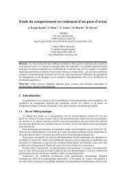
The aim of the present section is to evaluate the a priori performances of the Q4-DIC technique 

applied to the picture that corresponds to the reference configuration of the experiment to be 

analyzed in Section 4. Figure 2 shows the texture used to measure displacement fields. It is 

obtained by spraying a white and black paint prior to the experiment. Another picture (of 

stone wool) will also be analyzed. 

¢ 

0.03 

 

 

 

0.025 

¤¥¡£¡ 

¦§¡£¡ 

Frequency 

0.02 

0.015 

0.01 

¥¡£¡ 

0.005 

¨©¡£¡ 

¡¥¡£¡ 

¢¡£¡ ¤¥¡¥¡ ¦§¡£¡ ¨©¡£¡ ¡¥¡£¡ ¥¡¥¡ 

0 

1 2 3 4 5 

Gray level 

x 10 4 

Figure 2: View of a reference picture and corresponding gray level histogram. The tension axis 

is vertical. The width of the sample is 30 mm. 

3.1.1 Texture characteristics 

The quality of the displacement measurement is primarily based on the quality of the image 

texture. Hence before discussing the result of the analysis, the characteristics of the texture 

are presented. The gray level was encoded on a 16-bit depth (even though the original depth 

was equal to 12 bits) in the image acquisition, and the true gray level dynamic range takes 

advantage of this encoding, as judged from the gray level histogram shown in Fig. 2. Such a 

histogram is a good indication of the global image quality to check for saturation problems. 

However, such a global characterization of the image is only of limited interest. It is mostly 

useful at the stage of image acquisition to set, say, the exposure time and / or the aperture. 

Many acquisition softwares offer such functions. However, since the actual dynamic range of 

gray levels is an important element to appreciate the quality of a picture, it is included here as 

a possible diagnostic tool of poor performance. 

What is more significant is the average of texture properties as estimated from sampling of 

sub-images in elements. This is more a characteristic of the patterns than of image acquisition. 

The point is to evaluate whether the sub-images carry enough information to allow for a proper 

10

analysis. Each element is characterized by its own gray level dynamic range, or its standard 

deviation of gray level. The latter quantity, averaged over all elements of a given size, and 

normalized by the maximum gray level used in the image, is shown in Fig. 3-a. Even for the 

smallest element sizes, this ratio is already as large as 0.06, and increases to about 0.13 for large 

element sizes. The higher the ratio, the smaller the detection threshold as shown in Eq. (2); 

the standard deviation being an indirect way of characterizing the sensitivity of the technique. 

One thus concludes that the gray level amplitude is large enough to allow for a good quality of 

the analysis even for element sizes as small as 4 pixels. 

0.13 

3.5 

Mean gray level fluctuation 

0.12 

0.11 

0.1 

0.09 

0.08 

0.07 

x (pixel) 

3.0 

2.5 

2.0 

1.5 

0.06 

2 4 8 16 32 64 

Element size (pixel) 

1.0 

2 4 8 16 32 64 

Element size (pixel) 

-a- 

-b- 

Figure 3: Fluctuation of gray level values averaged over elements of different sizes normalized 

by the gray level dynamic range of the image (a). Average of largest (+) and smallest (◦) 

correlation radii determined on elements of varying sizes (b). 

Another significant criterion is the correlation radius of the image texture. The latter is 

computed from a parabolic interpolation of the auto-correlation function at the origin. The 

inverse of the two eigenvalues of the curvature give an estimate of the two correlation radii, ξ 1 

and ξ 2 , shown in Fig. 3-b when averaged over all elements of a given size. The texture is rather 

isotropic (i.e., similar eigenvalues), and remains small (varying from 1-2 to about 3 pixels) for 

all element sizes. This indicates a very good texture quality that reveals small scale details 

even for small element sizes. If one wants at least one disk and its complementary surrounding 

to get a good estimate, the correlation radii should be less than one fourth of the element size. 

This is achieved for element sizes greater than 6 pixels in the present case. 

11

How to get these results? 

To show the difference with a natural texture, another picture will be considered. It corresponds 

to that of a stone wool sample [10]. Choose the Texture option in the first menu. Another 

menu appears in which the format of the pictures has to be given (Fig. 4): 

• Unknown format: it should one of the following formats .bmp, .CR2, .hbf, .hmf, .jpg, 

.png, .tif. 

• Image .bmp: this is a classical 8-bit coded format. Make sure the pictures are stored as 

B/W .bmp files. 

• Image .hbf or Image .hmf: these are HOLO3 (www.holo3.com) formats. 

• Image .jpg: this is a classical 8-bit coded format. Make sure the pictures are stored as 

B/W .jpg files. 

• Image .png: this is a classical 8-bit coded format. Make sure the pictures are stored as 

B/W .png files. 

• Canon EOS 350: this is a .CR2 raw file. 

• Image .tif: this is a classical 8-bit or 16-bit coded format. Make sure the pictures are 

stored as B/W .tif files. 

Figure 4: Menu to choose the format of the picture and then the reference picture. 

The reference image, which is not necessarily located in the same directory as CORRELI Q4 , 

has to be chosen (Fig. 4). The next step consists in selecting the region of interest (ROI). Three 

options are possible: 

12

• Computation Click. Follow the instructions and click to choose the two end points of 

the ROI (Fig. 5). 

Figure 5: Choice of the Region Of Interest (ROI) by mouse click. Menu to choose the result 

file of a previous computation for which the same ROI will be considered. 

• Computation Restart. Indicate the results (.mat) file in which the ROI size is given 

(Fig. 5). 

• Computation Data. In the MATLAB Command Window, the user has to answer to four 

questions to choose the size of the ROI. The minimum and maximum values are given 

and they correspond to the image size: 

minimum horizontal coordinate 1

x 

Gray level histogram 

104 

2.5 

Region of interest 

2 

50 

Number of samples 

1.5 

1 

100 

150 

0.5 

200 

0 

120 130 140 150 160 170 180 

Gray level 

250 

50 100 150 200 250 

Figure 6: Histogram of the chosen ROI. 

believed that the measurement is not possible (i.e., there are not enough gradients to capture 

displacements). With this limit, it is concluded that about 30% of all 4-pixel elements do not 

meet this criterion. Such small size should therefore not be used. With 16-pixel and larger 

elements, this first criterion is always satisfied. 

100 

90 

80 

70 

Fluctuation criterion 

Unvalidated ZOI 

Validated ZOI 

0.04 

0.035 

0.03 

Mean fluctation 

Min. fluctation 

Limit 

ZOI percentage 

60 

50 

40 

30 

20 

Relative fluctuation 

0.025 

0.02 

0.015 

0.01 

10 

0.005 

0 

4 8 16 32 64 128 

ZOI size (pixels) 

0 

4 8 16 32 64 128 


Figure 7: Percentage of validated elements. Minimum and mean relative RMS fluctuations as 

functions of the element size in the analyzed picture of Fig. 6. 

Last, the principal correlation radii are shown in values expressed in pixels, and normalized 

by the element size (Fig. 8). A practical limit is chosen to be at most 25% of the element size. 

Above this value, it is believed that the measurement is not secure. With this limit, it is 

concluded that about 50% of all 8-pixel elements do not meet this criterion. Such small size 

should therefore not be used. With 16-pixel and larger elements, this second criterion is always 

satisfied. Last, let us note that the two correlation radii are significantly different. This result 

14

indicates that the texture is anisotropic (Fig. 6). The interested reader will find additional 

details in Ref. [18] concerning the determination of dominant orientations of a texture. 

ZOI percentage 

100 

90 

80 

70 

60 

50 

40 

30 

20 

Correlation radius criterion 

Unvalidated ZOI 

Validated ZOI 

Dimensionless correlation radii 

5 

4.5 

4 

3.5 

3 

2.5 

2 

1.5 

1 

R1mean 

R1max 

R2mean 

R2max 

Limit 

Correlation radii (pixels) 

20 

18 

16 

14 

12 

10 

8 

6 

4 

R1mean 

R1max 

R2mean 

R2max 

10 

0.5 

2 

0 

4 8 16 32 64 128 


0 

4 8 16 32 64 128 


0 

4 8 16 32 64 128 


Figure 8: Percentage of validated elements. Maximum and mean correlation radii as functions 

of the element size. 

With these two simple criteria, it is concluded that at least 16-pixel elements are to 

be chosen (i.e., both are satisfied simultaneously). It is worth noting that this first a priori 

analysis concerns only the texture itself. It is therefore a qualitative analysis. In the following, 

two quantitative analyses are proposed. 

3.1.2 Displacement uncertainty 

Prior to any computation, it is important to estimate the a priori performance of the approach 

on the actual texture of the image. If one changes the picture, one may not get exactly the 

same performance since it is related to the local details of the gray level distribution as shown 

in Section 2. This is performed by using the original image f only, and generating a translated 

image g by a prescribed amount u pre . Such an image is generated in Fourier space using a simple 

phase shift for each amplitude. This procedure implies a specific interpolation procedure for 

inter-pixel gray levels, to which one resorts systematically (see Section 2.3). The algorithm is 

then run on the pair of images (f, g), and the estimated displacement field u est (x) is measured. 

One is mainly interested in sub-pixel displacements, where the main origin of errors comes 

from inter-pixel interpolation. Therefore the prescribed displacement is chosen along the (1, 1) 

direction so as to maximize this interpolation sensitivity. To highlight this reference to the 

pixel scale, one refers to the x- (or y-) component of the displacement u pre ≡ u pre .e x varying 

from 0 to 1 pixel, rather than the Euclidian norm (varying from 0 to √ 2 pixel). 

The quality of the estimate is characterized by two indicators, namely, the systematic 

error, δ u = ‖〈u est 〉 − u pre ‖, and the standard uncertainty σ u = 〈‖u est − 〈u est 〉‖ 2 〉 1/2 . The 

change of these two indicators is shown in Fig. 9 as functions of the prescribed displacement 

amplitude for different element sizes l ranging from 4 to 128 pixels. Both quantities reach a 

15

maximum for one half pixel displacement, u pre = 0.5 pixel, and are approximately symmetric 

about this maximum. Integer valued displacements (in pixels) imply no interpolation and are 

exactly captured through the multi-scale procedure discussed above. This confirms that these 

errors are due to interpolation procedures. The results are shown in a semi-log scale to reveal 

the strong sensitivity to the element size, however a linear scale would show that both δ u and σ u 

follow approximately a linear increase with u pre from 0 to 0.5 pixel (and a symmetric decrease 

from 0.5 to 1 pixel). 

10 -1 0 0.2 0.4 0.6 0.8 1 

Mean displacement error (pixel) 

10 -2 

10 -3 

10 -4 

10 -5 

10 -6 

4 

8 

16 

32 

64 

128 

Standard uncertainty (pixel) 

10 0 0 0.2 0.4 0.6 0.8 1 

10 -1 

10 -2 

10 -3 

10 -4 

10 -5 

4 

8 

16 

32 

64 

128 

Prescribed displacement (pixel) 

Prescribed displacement (pixel) 

-a- 

-b- 

Figure 9: Mean error δ u and standard deviation σ u as a function of the prescribed displacement 

u pre for different element sizes l ranging from 4 to 128 pixels. 

To quantify the effect of the element size, the error and standard uncertainty, are averaged 

over u pre within the range [0, 1] as functions of the element size l. These data are shown in 

Fig. 10. A power-law decrease 

〈σ u 〉 = A 1+ζ l −ζ 

(14) 

〈δ u 〉 = B 1+υ l −υ 

for 8 ≤ l ≤ 128 pixels is usually observed as shown by a regression line on the graph. Both 

amplitudes are typically close to 1 pixel (more precisely A = 1.15 pixel and B = 1.07 pixel). 

The exponents are measured to be ζ = 1.96 and υ = 2.34. The data for l = 128 pixels seem 

to depart from the power-law trend with a tendency to saturate. These results quantify the 

trade-off the experimentalist has to face in the analysis of a displacement field, namely, either 

the measurement is accurate but estimated over a large zone, or it is spatially resolved but at 

the cost of a less accurate determination. This is a significant difference with classical finite 

element techniques for which convergence is achieved when the element size decreases. This 

is not the case when measurements are concerned. Let us however underline the following 

conclusions: 

16

© 

 

 

 

 

 

 

; 

 

 

 

 

: 

• Elements as small as l = 4 pixels may be used with an average error and standard 

uncertainty of the order of 0.1 pixel, 

• Systematic errors of the order of 10 −2 and 10 −3 pixel is reached for element sizes respectively 

equal to 8 and 16 pixels. 

• Standard uncertainties of the order of 2 × 10 −2 and 6 × 10 −3 pixel is reached for element 

sizes respectively equal to 8 and 16 pixels. 

• The systematic error in the determination of a displacement is such that evaluations will 

be “attracted” toward integer values. Correspondingly, transitions at half-integer pixel 

values for the displacement will appear as more abrupt. This phenomenon will be referred 

to as “integer locking” in the sequel, and will be discussed in detail. Let us underline 

that this spurious bias is revealed in this technique because the latter is used down to 

extremely small element sizes. 

¡ ¢ ¨ 

¡£¢ ¨ 

465 7 1'1"2-3 

3 465 7 89 

 

 

 

 

¡£¢§ 

¡£¢§ 

< 

¡£¢ ¦ 

¡£¢ ¦ 

¡£¢¥ 

 

¡£¢ ¤ 

¡£¢¥ 

¡ ¨ ¡ § 

¡ ¨ ¡ § 

"!$# % &')( *+% ,- . 

"!$# % &'=( *+% ,- . 

/ >$/ 

/ 0'/ 

Figure 10: Average error 〈δ u 〉 and standard uncertainty 〈σ u 〉 as functions of the element size 

l. For the displacement uncertainty, the results obtained by Q4-DIC are compared with those 

obtained by FFT-DIC. The dashed lines correspond to power-law fits. 

For comparison purposes, the displacement uncertainties obtained with the present technique 

are compared with those of a standard FFT-DIC technique [10]. In that case, a weaker 

power-law decrease is observed with A = 1.00 pixel and ζ = 1.23 (Fig. 10b). This result shows 

that by using a continuous description of the displacement field, it enables for a decrease of the 

displacement uncertainty when the same element size is used. Conversely, for a given displacement 

uncertainty, the Q4-DIC algorithm allows one to reduce significantly the element size, 

17

thereby increasing the number of measurement points when compared to a classical FFT-DIC 

technique. 


The same instructions as presented for the texture analysis (Section 3.1.1) hold. We reproduce 

them for a more linear reading. Choose the Uncertainty option in the first menu. Another 

menu appears in which the format of the pictures is chosen (Fig. 4): 


.png, .tif. 

















(Fig. 5). 




18


`U X 

^ T 

R _ 

]\\X 

\ 

ZX 

[ 

U VW 

YX 

 

¢¡¤£ ¥¡§¦ ¢¡©¨ 

¢¡¤ 

K Y 

Q ZN 

T W 

X M 

VQ 

TO 

K S 

J K LM 

N OP 

¢¡¤£ 

! #"#$!%'&)( *+-, .0/¤1325476 

¢¡¤£ ¥¡§¦ ¢¡©¨ 

¢¡¤ 

!.0/¤132405'6 798§:= 

"!#$ 

%'&)( *+-, 

 

[]\§^ _`_ 

¢¡¤¦ 

¢¡¤ ¨ 

¢¡¤¦ 

T U 

PS 

RQ 

SQ 

¢¡ 

¢¡ ¨ 

Q R ST 

?@BACDFE¤GBHIJDFKLGNMOCP 

89;:=@?¤A;BCD=@EFAHG#I 

Figure 12: Mean displacement error and standard deviation as functions of the element size. 

3.1.3 Noise sensitivity 

Last, the effect of noise associated to the image acquisition (e.g., digitization, read-out noise, 

black current noise, photon noise [20]) on the displacement measurement is assessed. This analysis 

allows one to estimate the displacement resolution [21]. The reference image is corrupted 

by a Gaussian noise of zero mean and standard variation σ g ranging from 1 to 8 gray levels 

at each pixel with no spatial correlation. No displacement field is superimposed on the image, 

and the displacement field is then estimated. The standard deviation of the displacement field, 

σ u , is shown in Fig. 13 as a function of the noise amplitude σ g and for different element sizes 

ranging from 4 to 128 pixels. The quantity σ u is linear in the noise amplitude and inversely proportional 

to the element size. The latter properties are derived from the central limit theorem. 

A theoretical analysis of this problem is discussed in Refs. [11, 22], and leads to the 

following estimate of the standard deviation of the displacement field induced by a Gaussian 

white noise 

σ u = 

12√ 2σ g p 

7〈|∇f| 2 〉 1/2 l 

where p is the physical pixel size. For the present application, one computes 〈|∇f| 2 〉 1/2 ≈ 

5340 pixel −1 , hence σ u ≈ 4.5 × 10 −4 σ g p/l. This theoretical expectation (neglecting the spatial 

correlation in the image texture) is consistent with the direct estimates shown in Fig. 13 (e.g., 

for l = 4 pixels and σ g = 8 gray levels, the direct estimate is 1.2×10 −3 pixel to be compared with 

9 × 10 −4 pixel given by the above formula). In practice, with the used CCD camera, the noise 

level is given with a maximum range less than 3 gray levels. Consequently, the contribution of 

(15) 

20

-3 

1.5 x 10 Noise level (gray level) 

Standard uncertainty (pixel) 

1 

0.5 

0 

0 2 4 6 8 

4 

8 

16 

32 

64 

128 

Figure 13: Standard deviation of the displacement error versus noise amplitude for different 

element sizes (4, 8, 16, 32, 64 and 128 pixels) from top to bottom. 

image noise is negligibly small when compared to that induced by the sub-pixel interpolation. 


The same instructions as presented for the texture analysis (Section 3.1.1) hold. We reproduce 

them for a more linear reading. Choose the Resolution option in the first menu. Another 

menu appears in which the format of the pictures has to be chosen (Fig. 4): 


.png, .tif. 











21







(Fig. 5). 





92 

+ 

65 

0 

)*+ 

*-, 

./+ 

32 

, 

),+' 

, 

),+' 

¦¥£ 

¦¥¤ 

¦¥¡ 

¦¥¢ 

§ 

4 7 

6:;5 

5 

67 

§¦ ¢ 

. 8 

234 

-1 

7 1 

§¦ 

§¦ ¡ 

/0 

%. 

2 3-+ 

+4 

-' 

%& 

§¦ ©¨ 

0.,1 

(* 

$%& 

(&' ) 

8:9 

¡ ¢ £ ¤ 

¥ §¦ ©¨ 

74; 695 

¡ ¢ £ ¤ 

¨©¦ !¦#" 

§! #"%$&§(' 

Figure 14: Mean displacement error and standard deviation as functions of the noise level for 

different element sizes. 

4 5 

§¡©¤ 

687 

/0 

-1 

%. 

-' 

%& 

§¡ ¨£ 

9 : 

(* 

$%& 

(&' ) 

¢¡£ ¤ ¤¥¡£ ¦ 

©§¥ !©§#" 

Figure 15: Mean displacement error and standard deviation as functions of the noise level for 

different element sizes. 

low noise features. Otherwise, it might be desirable to increase the element size, or work harder 

to get pictures with a better quality (this is, unfortunately not always possible...). 

3.2 Computation 

Any of the following options has to be selected to run directly a computation: 




(Fig. 5). 


23




• The number of scales is the second most important parameter. As discussed above, the 

present algorithm is based upon a coarse-graining approach. When large displacements 

and / or strains are suspected to occur, it is desirable to increase the number of scales. 

The maximum number of scales depends on the size of the ROI in comparison to that 

of the elements (e.g., for a 512 × 512pixel-ROI, and 16-pixels elements, the maximum 

number of scales is 5, i.e., at least 2 × 2 elements are needed for the coarsest scale). 

• The number of iterations (the higher the number, the higher the accuracy and the computation 

time). This value is given to avoid endless iterations. This criterion should not 

be reached. In case it is reached a message warns the user: 

--------------------------- WARNING - WARNING ----------------------------- 

Warning: No convergence: check results!! 

--------------------------- WARNING - WARNING ----------------------------- 

• The number of images to analyze (the reference image is not included in that count); 

• When a sequence of more than one image is considered, the correlation can be performed 

either by considering always the same reference image for strains (in absolute value) less 

than or equal to 10% or by changing (or updating) the reference image. In the last case, 

the Image update Y/N has to be activated. 

• Last, it is possible to store the correlation results for any couple of analyzed pictures. 

This is made possible by activating the Independent calculation Y/N button. 

Validate the choice at the end (press the Validation button). 

The sequence of deformed pictures has to be selected. The user selects the whole sequence 

by using the same procedure as for the reference picture (Fig. 17). 

It is then possible to mask part of the ROI. A menu appears and seven different operations 

are possible: 

• Define exclusion polygon allows the user by mouse click to enter different exclusion 

regions. Follow the instructions on top of the picture that appears. 

• Remove polygon allows the user by mouse click to remove any of the existing exclusion 

polygon. 

25

• Define exclusion circle allows the user, for instance to mask a hole. 

instructions on top of the picture that appears. 

Follow the 

• Remove exclusion circle allows the user by mouse click to remove any of the existing 

exclusion circle. 

• Define inclusion circle allows the user to choose a circular ROI from a rectangular 

shape chosen before. This would be the case for the analysis of a Brazilian test [12]. 

Follow the instructions on top of the picture that appears. 

• Remove inclusion circle allows the user by mouse click to remove any of the existing 

inclusion circle. 

• Redraw when the user is not happy with the (random) colors. 

• Exit to end the mask procedure. 

When the computation is completed, the result file has to be saved (Fig. 18). The extension 

is ‘.mat’ to be readable for a later visualization. The computation is now ended and the 

visualization stage starts. One can choose to perform another computation or to visualize any 

Figure 16: dialog box for choosing the correlation parameters. 

26

Figure 17: dialog box to choose the deformed picture(s). 

Figure 18: dialog box to choose the type of mask and to save the results 

results. Type the command correli_q4 at the MATLAB prompt. It can be noted that during 

the computations, different messages may appear. Some messages are only given to indicate 

that the computation is running normally. 

3.3 Visualization 

If Visualization is chosen, the result file (‘.mat’ extension) to be displayed has to be selected 

(Fig. 19). 

Figure 20 appears, in which different options can be chosen. In the present case, the 

vertical displacement field (expressed in pixels) is plotted for the stone wool texture for which 

an artificially deformed picture was created. A uniform nominal strain level of 0.25 was applied. 

This is an extreme case for the present correlation software that needs all the scales to capture 

properly the displacement field. The element size was equal to 16 pixels. It is worth noting 

that the maximum displacements are greater than 3 times the element size. Had the multiscale 

algorithm not been implemented, it would have been impossible to capture these levels (i.e., 5 

27

Figure 19: dialog box to read the results of a previous computation. 

scales were used in the present case). When a sequence is analyzed, any image can be selected 

Figure 20: Visualization of the measurement results. In the present case, the displacement field 

along the vertical direction. 

by using the two buttons bellow the Image No. message (Fig. 20). 

28

At the top left corner are options related to the strain measures: 

• infinitesimal: infinitesimal strains (i.e., symmetric part of displacement gradient, see 

Eq. (24)); 

• nominal: nominal (Cauchy-Biot) strains (Eq. (58), when m = 1/2); 

• Green Lag.: Green-Lagrange strains (Eq. (58), when m = 1); 

• logarithmic: logarithmic (Hencky) strains (Eq. (58), when m → 0 + ); 

• RdB (internal development); 

• Eigen value?: the eigen values of the selected strain measure are shown. 

It is worth noting that in the case of large strains (see details in the Appendix), the out-ofplane 

displacement is assumed to be small and is therefore neglected. Other assumptions can 

be made. They will have to be implemented on demand. 

Just below are options related to the type of component to visualize. The type of component 

to display has to be chosen, namely, in-plane strains, in-plane displacements, or out-ofplane 

rotation. The frame is always the same, namely, horizontal direction: 2, vertical direction: 

1. By choosing error, an error indicator (i.e., correlation residual |u(x).∇f(x) + f(x) − g(x)| 

normalized by the dynamic range of the picture) of the result is plotted. The closer to 0, the 

better the result (when no lighting variations occur, levels below few percentages are usually 

achieved). 

Two pictures are plotted. The left picture is always the very first reference picture. For 

the reference image, the chosen field is plotted. In the case of displacements, the average value 

is always in the middle of the scale. To change the scale, the dialog box in between the two 

images is to be used (Fig. 21). 

The number of contours can be changed. If 0 is set, a grayscale is used. If 11 is chosen, 

a fancy color scale appears, otherwise a conventional (i.e., hot) one is used. The amplitude of 

the displacement field is chosen with respect to the average value. For strains, two routes can 

be followed: 

• the maximum and minimum values are given by the user in the middle part of the dialog 

box; 

• the w or w/o mean button is activated and the average value corresponds to the middle 

of the scale, the range of which is chosen as the maximum strain. 

29

Figure 21: Contour and scale options. Mesh options. Amplification of the displacements. 

When the fill option is activated, the contours are filled on the reference image. The rigid 

body motion can be subtracted to the overall displacement by pushing the corresponding button 

(Rigid body motion Y/N). When the error indicator is plotted, there is no need to change any 

scale parameters, it is performed automatically. The w or w/o mean button can also be used. 

When selecting mesh, the undeformed and deformed meshes appear on the relevant images 

(Fig. 22). When selecting vector, the displacement vectors are shown (Fig. 21). It can be noted 

that both options can be used simultaneously. A slider enables the displacements to be amplified 

by a factor that can be chosen by the user (Fig. 21). When the amplification is greater than 1, 

the underlying image disappears. 

To further comment on the results on the artificially deformed picture, the corresponding 

(nominal) strain field is shown in Fig. 22. Since the w or w/o mean button is activated, the 

average strain can be read directly as the median value (i.e., 0.2396 ≈ 0.24 for a prescribed 

value of 0.25). 

3.4 Virtual Gauges 

Type the command gauge at the MATLAB prompt. This procedure allows for the computation 

of the average strain in a user-selected ROI. one needs to indicate the result file in which all 

the data needed are stored. Then the Region Of Interest (ROI) is selected by mouse. Click and 

maintain to select the ROI. If the ROI is larger than the mesh, then the size is automatically 

reset to the maximum size. 

In the MATLAB Command Window, average values of different strain tensors are given. 

30

Figure 22: Visualization of post-processed results. In the present case the normal (nominal) 

strains along the vertical direction. 

The corresponding eigen strains are also computed. The results can also be saved in an ASCII 

file. The computation is now ended. Type any command at the MATLAB prompt. 

4 Application to a tensile test 

In this section, an application of the previously proposed algorithm is carried out to analyze 

a tensile test performed on an aluminum alloy sample. In the plastic regime, the formation 

of localization strain bands is observed. The fact that for a given displacement uncertainty, 

smaller element sizes can be chosen in the present case (Q4-DIC) when compared with those 

of a standard FFT-DIC technique (Fig. 10b), enables one to better capture kinematic details 

in the localization band. 

31

4.1 Material and method 

The studied aluminum alloy is of type 5005 (i.e., more than 99 wt% of Al content and a small 

amount of Mg; these values were determined by electron probe micro-analysis). As shown in 

Fig. 2, the sample is a coated with sprayed black and white paints to create the random texture 

for the displacement field measurement. The sample size is 140 × 30 × 2 mm 3 . It is positioned 

within hydraulic grips of a 100 kN servo-hydraulic testing machine. Its alignment is checked 

with DIC measurements (i.e., no significant rotation of the sample is observed in the elastic 

domain). To have a first strain evaluation, an extensometer was used. Its pins are observed on 

the right edge of the sample (Fig. 2). 

An artificial light source is used to minimize gray level variations so that the conservation 

of the optical flow is considered as practically achieved. A CCD camera (12-bit digitization, 

noise less than 3 gray levels, resolution: 1024 × 1280 pixels) with a conventional zoom is 

positioned in front of the sample. In the present case, the physical size of one pixel is 25 µm. 

Two loading sequences are carried out. First, in the elastic domain, a controlled displacement 

rate of 5 µm/s is applied and pictures are taken for 12 µm-increments. Elastic properties may 

be identified [23]. This will not be discussed herein. Second, a controlled displacement rate of 

10 µm/s is applied to study strain localization and pictures are taken for 60 µm-increments. 

The following analysis of the displacement field is an increment between two image acquisitions 

in the “plastic” regime. 

Figure 23 shows the change of the average longitudinal strain with the number of pictures 

(or equivalently with time). This result was obtained by using the Q4-DIC analysis. Until the 

extensometer pins slipped (at about a 5% strain), the average strain measured by DIC and 

that given by the extensometer were close, even though the same surface was not analyzed. 

This response is typical of a Portevin-Le Châtelier (PLC) phenomenon or jerky flow [24]. 

From a microscopic point of view, PLC effects are related to dynamic interactions between 

mobile dislocations and diffusing solute atoms [25, 26]. From a macroscopic perspective, it is 

related to a negative strain rate sensitivity that leads to localized bands that are simulated [27]. 

Many experimental studies [28] however are based upon average strain measurements. There 

are also full-field displacement measurements performed by using, for instance, laser speckle 

interferometry [29]. Yet the spatial resolution did not allow for an analysis of the displacement 

field within the band. Additional insight is gained by using IR thermography [30]. 

32

¢¡ ¨§ 

¢¡ ¦© 

¢¡ ¨ 

¢¡ ¨ 

¢¡ 

 

¢¡ ¦¥ 

¢¡ ¤£ 

¥ © £ £¥ £© 

¤! "$#¨%'&)(#*,+¢&-% 

Figure 23: Mean strain for a region of interest of 1000 × 700 pixels as a function of the number 

of picture. The box shows the two pictures that are analyzed. 

4.2 Kinematic fields 

Let us now analyze the displacement field in between two states (0.3% mean strain apart, 

see Fig. 23). The same region of interest of size 1000 × 700 pixels is studied using the above 

method, with different element sizes ranging from 16 down to 4 pixels. Figures 24 and 25 show 

the resulting displacement fields (component U x and U y , respectively). Although the test is 

pure tension, the analysis reveals without ambiguity the presence of a localization band whose 

width is about 150 pixels, and across which the displacement discontinuity is about 2 pixels 

along the tension axis, and about 1 pixel perpendicular to it. Let us concentrate here on this 

single pair of images to validate the algorithm on a real experimental test and evaluate its 

performances. 

One notes that all element sizes may be used. As expected, the smallest element sizes are 

noisier, yet the agreement between all these determinations is excellent. Let us underline that 

FFT-DIC usually deals with element sizes equal or larger than 32 pixels, exceptionally 16 pixels 

for very favorable cases are used when locally constant displacement fields are sought. Using 

the Q4-DIC technique allows one to reduce the element size by a factor of 4, which means that 

the number of pixels in the element has been cut down by a factor of 16. 

Let us however note that one should be cautious about the fact that displacements have a 

tendency to be attracted toward integer values, especially for small element sizes. Therefore the 

direct evaluation of strains along the tension axis ε yy as obtained by the Q4P1-shape functions 

or equivalently as a simple finite difference is expected to be artificially increased at half-integer 

displacement components. Figure 26 shows such strain fields for 4 different element sizes from 

33

100 

100 

200 

200 

300 

300 

400 

400 

500 

500 

600 

600 

700 

700 

800 

200 400 600 

800 1000 

800 

200 400 600 

800 1000 

-a- 

-b- 

¢¡ £¥¤ ¦¨§ © 

100 

200 

300 

400 

500 

 

100 

0.4 

200 

0.2 

300 

0 

400 

0.2 

500 

600 

0.4 

600 

700 

0.6 

700 

800 

200 400 600 

800 1000 

800 

200 400 600 

800 1000 

-c- 

-d- 

100 

100 

200 

200 

300 

300 

400 

400 

500 

500 

600 

600 

700 

700 

800 

200 400 600 

800 1000 

800 

200 400 600 

800 1000 

-e- 

-f- 

Figure 24: Map of U y displacement for different element sizes: (a) l = 16, (b) l = 12, (c) 

l = 10, (d) l = 8, (e) l = 6 and (f) l = 4 pixels. The physical size of one pixel is equal to 

25 µm. 

16 down to 8 pixels. For a size of 16 pixels, the localization band appears as a genuine zone 

of increased strains as compared to a “silent” (or elastic) background. For smaller element 

sizes, the edges of the shear band appear to concentrate still a higher strain. The same effect 

is apparent for element sizes 12, 10 and 8 pixels. The strain maps obtained for smaller element 

sizes are not shown, since the noise level becomes much higher and thus the measurement 

cannot be trusted. The same artefact of strain enhancement at the edges of the shear band is 

however observed. 

34

100 

100 

200 

200 

300 

300 

400 

400 

500 

500 

600 

600 

700 

700 

800 

200 400 600 

800 1000 

800 

200 400 600 

800 1000 

-a- 

-b- 

£ ¥¦ ¨© 

100 

100 

¢¡¤£ ¥§¦ ¨§© 

200 

300 

400 

500 

600 

700 

2 

1.5 

1 

0.5 

0 

200 

300 

400 

500 

600 

700 

800 

200 400 600 

800 1000 

800 

200 400 600 

800 1000 

-c- 

-d- 

100 

100 

200 

200 

300 

300 

400 

400 

500 

600 

700 

800 

200 400 600 

800 1000 

500 

600 

700 

800 

200 400 600 

-e- 

-f- 

800 1000 

Figure 25: Map of U x displacement for different element sizes: (a) l = 16, (b) l = 12, (c) 

l = 10, (d) l = 8, (e) l = 6 and (f) l = 4 pixels. The physical size of one pixel is equal to 

25 µm. 

4.3 Integer locking 

One notes on the previous figure that the U y -displacement is half-integer valued at the edge of 

the shear band. The larger strains at the edge of the band could therefore be interpreted as an 

artefact due to integer locking. Integer valued displacements being favored, an artificial gap is 

created for half-integer values displacement, and thus any gradient (finite difference operator) 

will underline this effect very markedly. 

To test this interpretation, the following test is proposed. An artificially translated image 

by 0.5 pixel is computed from the original one, using a fast Fourier transform, as the latter 

35

100 

100 

200 

200 

300 

300 

400 

400 

500 

500 

600 

600 

700 

700 

800 

200 400 600 

800 1000 

800 

200 400 600 

800 1000 

-a- 

-b- 

y (pixel) 

ε xx 

x (pixel) 

100 

200 

300 

0.025 

0.02 

0.015 

100 

200 

300 

400 

500 

0.01 

0.005 

0 

400 

500 

600 

700 

800 

200 400 600 

800 1000 

0.005 

0.01 

0.015 

600 

700 

800 

200 400 600 

800 1000 

-c- 

-d- 

Figure 26: Map of the strain component ε xx for different element sizes: (a) l = 16, (b) l = 12, 

(c) l = 10 and (d) l = 8 pixels. 

provides a simple and numerically efficient way of interpolating the image at any arbitrary subpixel 

value. A genuine strain enhancement is thus expected to be identified at a fixed position 

in the reference image frame of coordinates, whereas a numerical artefact would be moved to 

a different location. Figures 27a and b show the U y displacement component starting from 

the original image or from the translated one (and where the 1/2 pixel translated has been 

corrected for). A good agreement is observed for the displacement field thus revealing a rather 

poor sensitivity to such a rigid translation. Figures 27c and d show the corresponding ε yy strain 

maps. On the latter set of figures, although high strain values tend to concentrate along two 

lines in both figures, the precise location of these bands is not stable. This is a signature of the 

integer locking phenomenon. Therefore the strain enhancement at the edge of the shear band 

is to be considered as an artefact. 

Let us underline that such a phenomenon results from the fact that the elements are 

reduced to a very small size, and still provide a very accurate determination of the displacement 

field, without much noise. Such a success encourages the user to decrease the size of the elements 

to very small values. By doing so, the determination of the displacement is much more prone 

36

U x (pixel) 

100 

200 

0 

100 

200 

300 

0.5 

300 

400 

500 

600 

1 

1.5 

400 

500 

600 

700 

2 

700 

800 

200 400 600 

800 1000 

800 

200 400 600 

800 1000 

-a- 

-b- 

y (pixel) 

ε xx 

x (pixel) 

100 

200 

0.04 

0.03 

100 

200 

300 

400 

500 

600 

0.02 

0.01 

0 

0.01 

0.02 

300 

400 

500 

600 

700 

0.03 

700 

800 0.04 

200 400 600 800 1000 

800 

200 400 600 

800 1000 

-c- 

-d- 

Figure 27: Map of U x displacement, estimated for a element size l = 12 pixels: (a) for the 

original image, (b) for an artificially translated image of 0.5 pixel. Maps of the corresponding 

normal strain component ε xx : (c) for the original image, (d) for an artificially translated image 

of 0.5 pixel. The physical size of one pixel is equal to 25 µm. 

to slight sub-pixel shifts (Fig. 10), here characterized as an attraction toward integer values, 

which appear as very significant upon differentiation (in the computation of the strain). This 

phenomenon should be identified before any further interpretation of the strain map to ensure 

its validity. 

4.4 Error maps 

As mentioned earlier, a very important output of the displacement measurement obtained from 

a minimization procedure is that the optimization functional provides not only a global quality 

factor of the determined field, but more importantly a spatial map of residuals, so that one 

may appreciate a specific problem that may be spatially localized. 

Figure 28 shows the different error maps obtained for different element sizes. This error 

is the remanent difference in gray levels that is still unexplained by the estimated displacement 

field. The first observation is that the error level does not vary very much with the element 

37

size. This is consistent with the fact that the displacement field is quite comparable for different 

element sizes. However, there is a slight increase in the error as the element size decreases. This 

is explained by the fact that the performance of the correlation algorithm degrades as the spatial 

resolution improves. This observation is in good agreement with the results to be expected from 

the analysis of Fig. 10. 

Figure 28: Map of the residual error η for different element sizes: (a) l = 16, (b) l = 12, (c) 

l = 10 (d) l = 8, (e) l = 6 and (f) l = 4 pixels. 

5 Applications of CORRELI Q4 

In the following, different references are given in which the software was used. The abstract is 

given for the reader to select the relevant ones. The name of the .pdf file is also given. 

38

5.1 Reference paper 

G. Besnard, F. Hild and S. Roux, “Finite-element” displacement fields analysis from digital 

images: Application to Portevin-Le Châtelier bands, Exp. Mech. 46 (2006) 789-803. EM2.pdf 

This is the paper in which the so-called Q4-DIC technique is discussed in details. A new 

methodology is proposed to estimate displacement fields from pairs of images (reference and 

strained) that evaluates continuous displacement fields. This approach is specialized to a finiteelement 

decomposition, therefore providing a natural interface with a numerical modeling of 

the mechanical behavior used for identification purposes. The method is illustrated with the 

analysis of Portevin-Le Châtelier bands in an aluminum alloy sample subjected to a tensile test. 

A significant progress with respect to classical digital image correlation techniques is observed 

in terms of spatial resolution and uncertainty. 

5.2 Identification of elastic properties 

F. Hild and S. Roux, Digital image correlation: from measurement to identification of elastic 

properties - A review, Strain 42 (2006) 69-80. Strain1.pdf 

The current state of the art of digital image correlation, where displacements can be determined 

for values less than one pixel, enables one to better characterize the behavior of materials 

and the response of structures to external loads. A general presentation of the extraction of 

displacement fields from pictures taken at different instants during an experiment is given. 

Different strategies can be followed to determine sub-pixel displacements. New identification 

procedures are then devised making use of full-field measurements. A priori or a posteriori 

routes can be followed. They are illustrated on the analysis of a Brazilian disk test. 

5.3 SIF measurements 

S. Roux and F. Hild, Stress intensity factor measurements from digital image correlation: postprocessing 

and integrated approaches, Int. J. Fract. 140 [1-4] (2006) 141-157. IJF4.pdf 

Digital image correlation is an appealing technique for studying crack propagation in 

brittle materials such as ceramics. A case study is discussed where the crack geometry, and 

the crack opening displacement are evaluated from image correlation by following two different 

measurement and identification routes. The displacement uncertainty can reach the nanometer 

range even though optical pictures are dealt with. The stress intensity factor is estimated with 

a 7% uncertainty in a complex loading set-up without having to resort to a numerical modeling 

of the experiment. 

39

R. Hamam, F. Hild and S. Roux, Stress intensity factor gauging by digital image correlation: 

Application in cyclic fatigue, Strain 43 (2007) 181-192. Strain2.pdf 

A fatigue crack in steel (CCT geometry) is studied via digital image correlation. The 

measurement of the stress intensity factor change during one cycle is performed using a decomposition 

of the displacement field onto a tailored set of elastic fields. The same analysis 

is performed using two different routes, namely, the first one consists in computing the displacement 

field using a general correlation technique providing the displacement field projected 

onto finite element shape functions, and then analyzing this displacement field in terms of the 

selected mechanically relevant fields. The second strategy, called integrated approach, directly 

estimates the amplitude of these elastic fields from the correlation of successive images. Both 

procedures give consistent results, and offer very good performances in the evaluation of the 

crack tip position (uncertainty of about 20 µm for a 14.5-mm crack), and stress intensity factors 

(uncertainty less than 1 MPa √ m). 

J. Réthoré, S. Roux and F. Hild, Noise-robust Stress Intensity Factor Determination from Kinematic 

Field Measurements, Eng. Fract. Mech. (2008) DOI: 10.1016/j.engfracmech.2007.04.018. 

EFM1.pdf 

Stress Intensity Factors are often estimated numerically from a given displacement field 

through an interaction integral formalism. The latter method makes use of a weight, the virtual 

crack extension field, which is under-constrained by first principles. Requiring a least noise 

sensitivity allows one to compute the optimal virtual crack extension. Mode I and mode II 

specialized fields are obtained and particularized for a given displacement functional basis. The 

method is applied to an experimental case study of a crack in a silicon carbide sample, whose 

displacement field is obtained by a digital image correlation technique. The optimization leads 

to a very significant uncertainty reduction up to a factor 100 of the non-optimized formulation. 

The proposed scheme reveals additional performances with respect to the integral domain choice 

and assumed crack tip geometry, which are shown to have a reduced influence. 

5.4 Analysis of elasto-plastic laws 

V. Tarigopula, O. S. Hopperstad, M. Langseth, A. H. Clausen, F. Hild, O.-G. Lademo and 

M. Eriksson, A Study of Large Plastic Deformations in Dual Phase Steel Using Digital Image 

Correlation and FE Analysis, Exp. Mech. 48 [2] (2008) 181-196. EXME3.pdf 

Large plastic deformation in sheets made of dual phase steel DP800 is studied experimentally 

and numerically. Shear testing is applied to obtain large plastic strains in sheet metals 

without strain localisation. In the experiments, full-field displacement measurements are car- 

40

ied out by means of digital image correlation, and based on these measurements the strain field 

of the deformed specimen is calculated. In the numerical analyses, an elastoplastic constitutive 

model with isotropic hardening and the Cockcroft-Latham fracture criterion is adopted to 

predict the observed behavior. The strain hardening parameters are obtained from a standard 

uniaxial tensile test for small and moderate strains, while the shear test is used to determine 

the strain hardening for large strains and to calibrate the fracture criterion. Finite Element 

(FE) calculations with shell and brick elements are performed using the non-linear FE code 

LS-DYNA. The local strains in the shear zone and the nominal shear stress-elongation characteristics 

obtained by experiments and FE simulations are compared, and, in general, good 

agreement is obtained. It is demonstrated how the strain hardening at large strains and the 

Cockcroft-Latham fracture criterion can be calibrated from the in-plane shear test with the aid 

of non-linear FE analyses. 

5.5 Identification of a damage law 

S. Roux and F. Hild, Digital Image Mechanical Identification (DIMI), Exp. Mech. DOI: 

10.1007/s11340-007-9103-3 (2008). EXME4.pdf 

A continuous pathway from digital images acquired during a mechanical test to quantitative 

identification of a constitutive law is presented herein based on displacement field analysis. 

From images, displacement fields are directly estimated within a finite element framework. 

From the latter, the application of the equilibrium gap method provides the means for rigidity 

field evaluation. In the present case, a reconditioned formulation is proposed for a better stability. 

Last, postulating a specific form of a damage law, a linear system is formed that gives a 

direct access to the (non-linear) damage growth law in one step. The two last procedures are 

presented, validated on an artificial case, and applied to the case of a biaxial tension of a composite 

sample driven up to failure. A quantitative estimate of the quality of the determination 

is proposed, and in the last application, it is shown that no more than 7% of the displacement 

field fluctuations are not accounted for by the determined damage law. 

5.6 Analyses of localized phenomena 

I. Elnasri, S. Pattofatto, H. Zhao, H. Tsitsiris, F. Hild and Y. Girard, Shock enhancement of 

cellular structures under impact loading: Part I Experiments, J. Mech. Phys. Solids 55 (2007) 

2652-2671. JMPS2.pdf 

This paper aims at showing experimental proof of the existence of a shock front in cellular 

structures under impact loading, especially at low critical impact velocities around 50 m/s. 

41

First, an original testing procedure using a large diameter Nylon Hopkinson bar is introduced. 

With this large diameter soft Hopkinson bar, tests under two different configurations (pressure 

bar behind/ahead of the supposed shock front) at the same impact speed are used to obtain the 

force/time histories behind and ahead of the assumed shock front within the cellular material 

specimen. Stress jumps (up to 60% of initial stress level) as well as shock front speed are measured 

for tests at 55 m/s on Alporas foams and nickel hollow sphere agglomerates, whereas no 

significant shock enhancement is observed for Cymat foams and 5056 aluminium honeycombs. 

The corresponding rate sensitivity of the studied cellular structures is also measured and it 

is proven that it is not responsible for the sharp strength enhancement. A photomechanical 

measurement of the shock front speed is also proposed to obtain a direct experimental proof. 

The displacement and strain fields during the test are obtained by correlating images shot with 

a high speed camera. The strain field measurements at different times show that the shock 

front discontinuity propagates and allows for the measurement of the propagation velocity. All 

the experimental evidences enable us to confirm the existence of a shock front enhancement 

even at quite low impact velocities for a number of studied materials. 

V. Tarigopula, O. S. Hopperstad, M. Langseth, A. H. Clausen and F. Hild, A study of localisation 

in dual phase high-strength steels under dynamic loading using digital image correlation 

and FE analysis, Int. J. Solids Struct. 45 [2] (2008) 601-619. IJSS5.pdf 

Tensile tests were conducted on dual-phase high-strength steel in a Split-Hopkinson Tension 

Bar at a strain-rate in the range of 150600/s and in a servo-hydraulic testing machine at a 

strain-rate between 10 −3 and 100/s. A novel specimen design was utilized for the Hopkinson bar 

tests of this sheet material. Digital image correlation was used together with high-speed photography 

to study strain localisation in the tensile specimens at high rates of strain. By using 

digital image correlation, it is possible to obtain in-plane displacement and strain fields during 

non-uniform deformation of the gauge section, and accordingly the strains associated with diffuse 

and localized necking may be determined. The full-field measurements in high strain-rate 

tests reveal that strain localisation started even before the maximum load was attained in the 

specimen. An elasto-viscoplastic constitutive model is used to predict the observed stressstrain 

behavior and strain localisation for the dual-phase steel. Numerical simulations of dynamic 

tensile tests were performed using the non-linear explicit FE code LS-DYNA. Simulations were 

done with shell (plane stress) and brick elements. Good correlation between experiments and 

numerical predictions was achieved, in terms of engineering stressstrain behavior, deformed geometry 

and strain fields. However, mesh density plays a role in the localisation of deformation 

in numerical simulations, particularly for the shell element analysis. 

42

6 Beyond CORRELI Q4 

In the following, different references are given in which extensions of the software were used. 

The abstract is given for the reader to select the relevant ones. 

6.1 XQ4-DIC 

J. Réthoré, F. Hild and S. Roux, Shear-band capturing using a multiscale extended digital 

image correlation technique, Comp. Meth. Appl. Mech. Eng. 196 [49-52] (2007) 5016-5030. 

CMAME2.pdf 

Finite elements have been used recently to solve the optical flow conservation principle 

invoked to determine displacement fields by digital image correlation. Inspired by these recent 

advances, and by the computational effort that has been accomplished during the past 10 

years for the simulation of discontinuities by the extended finite element method (XFEM), an 

extended correlation technique is introduced for capturing shear-band like discontinuities from 

images of real mechanical tests. Because of the specific information at hand (i.e., gray level 

images), this extended finite element approach is included in a non-linear multi-grid solver. The 

performances of the proposed approach are discussed on two examples, namely the analysis of 

a bolted assembly and the formation of Piobert-Lüders bands. 

J. Réthoré, G. Besnard, G. Vivier, F. Hild and S. Roux, Experimental investigation of localized 

phenomena using Digital Image Correlation, Phil. Mag. [submitted] (2008). PM1.pdf 

The present paper is dedicated to the use of enriched discretization schemes in the context 

of digital image correlation. The aim is to capture and evaluate strong or weak discontinuities 

of a displacement field directly from digital images. An analysis of different enrichment performances 

is provided. Two examples of strain localization illustrate the discussion, namely, 

a compression test on an HMX-based material and the Portevin-Le Châtelier band shown in 

Section 4. 

J. Réthoré, F. Hild and S. Roux, Extended digital image correlation with crack shape optimization, 

Int. J. Num. Meth. Eng. 73 [2] (2008) 248-272. IJNME2.pdf 

The methodology of eXtended finite element method is applied to the measurement of displacements 

through digital image correlation. An algorithm, initially based on a finite element 

decomposition of displacement fields, is extended to benefit from discontinuity and singular enrichments 

over a suited subset of elements. This allows one to measure irregular displacements 

encountered, say, in cracked solids, as demonstrated both in artificial examples and experi- 

43

mental case studies. Moreover, an optimization strategy for the support of the discontinuity 

enables one to adjust the crack path configuration to reduce the residual mismatch, and hence 

to be tailored automatically to a wavy or irregular crack path. 

6.2 Beam-DIC 

F. Hild, S. Roux, R. Gras, N. Guerrero, M. E. Marante and J. Flórez-López, Displacement 

Measurement Technique for Euler-Bernoulli Kinematics, Opt. Lasers Eng. [accepted] (2008). 

OLE1.pdf 

It is proposed to develop a digital image correlation procedure that is suitable for beams 

whose kinematics is described by an Euler-Bernoulli hypothesis. As a direct output, the degrees 

of freedom corresponding to flexural and axial loads are directly measured. The performance 

of the correlation algorithm is evaluated by using a picture of a cantilever beam experiment. 

One load level is analyzed with the present algorithm. The latter is validated by comparing the 

displacement field with that given by a finite element based correlation algorithm. It is also 

shown that a locally buckled zone is detectable with the present procedure. 

6.3 Stereo-correlation 

G. Besnard, F. Hild, J.-M. Lagrange, S. Roux and C. Voltz, Contact-free characterization of 

materials used in detonics experiments, Proceedings Europyro 2007 . EUROPYRO_07.pdf 

In detonics experiments, specimens are loaded through intense shock waves produced by 

explosives, and hence the simultaneous occurrence of large strains and high strain rates makes 

the analysis delicate. Attention is here focused on tantalum whose elasto-plastic properties are 

quite complex, possibly involving strain localization. In order to face this challenge, the choice 

has been made to use imaging techniques, both for quasi-static tests (few images per second 

at most) and dynamic experiments (up to one million frames per second). Displacement fields 

are analyzed through digital image correlation techniques applied to monovision for in-plane 

displacements, and stereocorrelation when the three dimensional components of the surface 

displacement field are sought. Quasi-static tests on a tantalum specimen give access to the 

elastic properties (Young’s modulus and Poisson’s ratio), but also reveal strain localization 

occurring in the plastic flow regime. Extension of this technique to stereocorrelation is underway 

in order to have access to microsecond time resolution, and sub-millimeter space resolution. 

44

6.4 C8-DIC 

S. Roux, F. Hild, P. Viot and D. Bernard, Three dimensional image correlation from X-Ray 

computed tomography of solid foam, Comp. Part A DOI: 10.1016/j.compositesa.2007.11.011 

[in press] (2008). CompPartA1.pdf 

A new methodology is proposed to estimate 3D displacement fields from pairs of images 

obtained from X-Ray Computed Micro Tomography (XCMT). Contrary to local approaches, 

a global approach is followed herein that evaluates continuous displacement fields. Although 

any displacement basis may be considered, the procedure is specialized to finite element shape 

functions. The method is illustrated with the analysis of a compression test on a polypropylene 

solid foam (independently studied in a companion paper). A good stability of the measured 

displacement field is obtained for cubic element sizes ranging from 16 voxels to 6 voxels. This 

last paper is a direct extension of Q4-DIC to three-dimensional displacement measurements in 

the bulk of a material. 

7 Conclusion 

A novel approach was developed to determine a displacement field based on the comparison 

of two digital images. The sought displacement field is decomposed onto a basis of continuous 

functions using Q4P1-shape functions as proposed in finite element methods. The latter corresponds 

to one of the simplest kinematic descriptions. It therefore allows for a compatibility of 

the kinematic hypotheses made during the measurement stage and the subsequent identification 

/ validation stage, for instance, by using conventional finite element techniques. 

The performance of the algorithm is tested on a reference image to evaluate the reliability 

of the estimation, which is shown to allow for either an excellent accuracy for homogeneous 

displacement fields, or for a very well resolved displacement field down to element sizes as small 

as 4×4 pixels. When compared with a standard FFT-DIC technique, Q4-DIC enables for a 

significant decrease of the displacement uncertainty when the same size of the elements is used. 

For the natural texture studied herein, it is shown that the main limitation is related to its 

poor dynamic range that makes it very sensitive to acquisition noise. 

Last, the displacement field is analyzed on an aluminium alloy sample where a localization 

band develops. In the present case, it corresponds to a Portevin-Le Châtelier effect. For element 

sizes ranging from 16 down to 4 pixels, the displacement field is shown to be reliably determined. 

As far as strains are concerned, spurious strain concentrations at the edge of the shear band 

is observed for small element sizes. This is attributed to integer locking of the displacement. 

Apart from this bias, the analysis has been shown to be operational and reliable, on a real 

45

experimental test with strain localization. The complete space-time kinematic analysis is now 

possible for the Portevin-Le Châtelier phenomenon even within the band thanks to the spatial 

resolution achieved by the Q4-DIC technique presented herein. It is deferred to a another 

publication in which an enriched kinematics is implemented [31]. 

References 

[1] P. K. Rastogi, edts., Photomechanics, (Springer, Berlin (Germany), 2000), 77. 

[2] M. A. Sutton, S. R. McNeill, J. D. Helm and Y. J. Chao, Advances in Two-Dimensional and 

Three-Dimensional Computer Vision, in: Photomechanics, P. K. Rastogi, eds., (Springer, 

Berlin (Germany), 2000), 323-372. 

[3] A. Lagarde, edt., Advanced Optical Methods and Applications in Solid Mechanics, 

(Kluwer, Dordrecht (the Netherlands), 2000), 82. 

[4] O. C. Zienkievicz and R. L. Taylor, The Finite Element Method, (McGraw-Hill, London 

(UK), 4th edition, 1989). 

[5] B. K. P. Horn and B. G. Schunck, Determining optical flow, Artificial Intelligence 17 

(1981) 185-20. 

[6] P. J. Hubert, Robust Statistics, (Wiley, New York (USA), 1981). 

[7] M. Black, Robust Incremental Optical Flow, (PhD dissertation, Yale University, 1992). 

[8] J.-M. Odobez and P. Bouthemy, Robust multiresolution estimation of parametric motion 

models, J. Visual Comm. Image Repres. 6 (1995) 348-365. 

[9] M. A. Sutton, W. J. Wolters, W. H. Peters, W. F. Ranson and S. R. McNeill, Determination 

of Displacements Using an Improved Digital Correlation Method, Im. Vis. Comp. 1 [3] 

(1983) 133-139. 

[10] F. Hild, B. Raka, M. Baudequin, S. Roux and F. Cantelaube, Multi-Scale Displacement 

Field Measurements of Compressed Mineral Wool Samples by Digital Image Correlation, 

Appl. Optics IP 41 [32] (2002) 6815-6828. 

[11] S. Roux and F. Hild, Stress intensity factor measurements from digital image correlation: 

post-processing and integrated approaches, Int. J. Fract. 140 [1-4] (2006) 141-157. 

46

[12] F. Hild and S. Roux, Digital image correlation: from measurement to identification of 

elastic properties - A review, Strain 42 (2006) 69-80. 

[13] F. Hild, S. Roux, R. Gras, N. Guerrero, M. E. Marante and J. Flórez-López, Displacement 

Measurement Technique for Euler-Bernoulli Kinematics, Opt. Lasers Eng. [accepted] 

(2008). 

[14] B. Wagne, S. Roux and F. Hild, Spectral Approach to Displacement Evaluation From 

Image Analysis, Eur. Phys. J. AP 17 (2002) 247-252. 

[15] S. Roux, F. Hild and Y. Berthaud, Correlation Image Velocimetry: A Spectral Approach, 

Appl. Optics 41 [1] (2002) 108-115. 

[16] P. J. Burt, C. Yen and X. Xu, Local correlation measures for motion analysis: a comparative 

study, Proceedings IEEE Conf. on Pattern Recognition and Image Processing, (1982), 

269-274. 

[17] H. W. Schreier, J. R. Braasch and M. A. Sutton, Systematic errors in digital image correlation 

caused by intensity interpolation, Opt. Eng. 39 [11] (2000) 2915-2921. 

[18] S. Bergonnier, F. Hild and S. Roux, Local anisotropy analysis for non-smooth images, 

Patt. Recogn. 40 [2] (2007) 544-556. 

[19] J.-N. Périé, S. Calloch, C. Cluzel and F. Hild, Analysis of a Multiaxial Test on a C/C 

Composite by Using Digital Image Correlation and a Damage Model, Exp. Mech. 42 [3] 

(2002) 318-328. 

[20] G. Holst, CCD Arrays, Cameras and Displays, (SPIE Engineering Press, Washington DC 

(USA), 1998). 

[21] ISO, International Vocabulary of Basic and General Terms in Metrology (VIM), (International 

Organization for Standardization, Geneva (Switzerland), 1993). 

[22] G. Besnard, F. Hild and S. Roux, “Finite-element” displacement fields analysis from digital 

images: Application to Portevin-Le Châtelier bands, Exp. Mech. 46 (2006) 789-803. 

[23] G. Besnard, Corrélation d’images et identification en mécanique des solides, (University 

Paris 6, Intermediate MSc report 2005). 

[24] A. Portevin and F. Le Châtelier, C. R. Acad. Sci. Paris 176 (1923) 507. 

[25] A. H. Cottrell, A note on the Portevin-Le Châtelier effect, Phil. Mag. 44 (1953) 829-832. 

47

[26] P. G. McCormick, A model of the Portevin-Le Châtelier effect in substitutional alloys, 

Acta Metall. 20 (1972) 351-354. 

[27] A. H. Clausen, T. Borvik, O. S. Hopperstad and A. Benallal, Flow and fracture characteristics 

of aluminium alloy AA5083-H116 as function of strain rate, temperature and 

triaxiality, Mat. Sci. Eng. A364 (2004) 260-272. 

[28] D. Thevenet, M. Mliha-Touati and A. Zeghloul, Characteristics of the propagating deformation 

bands associated with the Portevin-Le Châtelier effect in an Al-Zn-Mg-Cu alloy, 

Mat. Sci. Eng. A291 (2000) 110-117. 

[29] R. Shabadi, S. Kumara, H. J. Roven and E. S. Dwarakadasa, Characterisation of PLC 

band parameters using laser speckle technique, Mat. Sci. Eng. A364 (2004) 140-150. 

[30] H. Louche, P. Vacher and R. Arrieux, Thermal observations associated with the Portevin- 

Le Châtelier effect in an Al-Mg alloy, Mat. Sci. Eng. A 404 (2005) 188-196. 

[31] J. Réthoré, G. Besnard, G. Vivier, F. Hild and S. Roux, Experimental investigation of 

localized phenomena using Digital Image Correlation, Phil. Mag. [submitted] (2008). 

[32] R. Hill, Aspects of Invariance in Solid Mechanics, Adv. Appl. Mech. 18 (1978) 1-75. 

48

Appendix: Strain measures 

From the displacement field, the strain field is usually sought. Different strain measures can be 

used to analyze a mechanical experiment. 

7.1 Infinitesimal strains 

A strain is defined in terms of relative variation of length of a line linking two material points 

of a deformable body. This intuitive definition will be completed in the following subsections. 

The displacement of a point P (x, y, z) is defined by three components (u, v, w) of a vector u in 

a cartesian coordinate system chosen in the undeformed state 

A second point Q in the vicinity of P moves to Q ′ 

P (x, y, z) → P ′ (x + u, y + v, z + w) (16) 

Q(x + dx, y + dy, z + dz) → 

Q ′ (x + dx + u + du, y + dy + v + dv, z + dz + w + dw) (17) 

The quantities du, dv, dw are called relative displacements. When du, dv, dw are sufficiently 

small (i.e., infinitesimal) compared to the length scale dx, dy, dz, a first order approximation 

of the variations du, dv, dw can be written as 

du = ∂u 

∂x 

dv = ∂v 

∂x 

dw = ∂w 

∂x 

∂u ∂u 

dx + dy + 

∂y ∂z dz 

dx + 

∂v 

∂y 

The previous equation can be written in matrix form 

∂v 

dy + dz (18) 

∂z 

∂w ∂w 

dx + dy + 

∂y ∂z dz. 

du = gradu dx (19) 

Of the nine components obtained in Eqn. (18), they are grouped as follows for the normal 

strains 

for the shear strains 

ε xx = ∂u 

∂x , ε yy = ∂v 

∂y 

ε xy = ε yx = 1 ( ∂u 

2 ∂y + ∂v ) 

∂x 

ε yz = ε zy = 1 ( ∂v 

2 ∂z + ∂w ) 

∂y 

ε zx = ε xz = 1 ( ∂w 

2 ∂x + ∂u ) 

∂z 

49 

, ε zz = ∂w 

∂z 

(20) 

(21)

and the infinitesimal rotations 

ω z = 1 ( 

− ∂u 

2 ∂y + ∂v ) 

∂x 

ω x = 1 ( 

− ∂v 

2 ∂z + ∂w ) 

∂y 

ω y = 1 ( 

− ∂w 

2 ∂x + ∂u ) 

∂z 

These results are related to the symmetric and antisymmetric decomposition of the gradient 

operator 

(22) 

gradu = grad s u + grad a u (23) 

where the infinitesimal strain tensor ε is defined by 

ε = grad s u = 1 ( 

gradu + grad t u ) (24) 

2 

and the infinitesimal rotation tensor Ω is expressed as 

Ω = grad a u = 1 ( 

gradu − grad t u ) (25) 

2 

It can be shown that an antisymmetric tensor can be related to a vector (here the rotation 

vector ω) by 

Examples: 

Ωdx = ω × dx (26) 

Let us first consider a rigid translation. The two points P and Q then move by an identical 

amount u 

P → P ′ (x + u, y + v, z + w) 

Q → Q ′ (x + dx + u, y + dy + v, z + dz + w) (27) 

so that the displacement gradient vanishes, so do the strains and the rotation vector. 

The second example deals with a small rigid rotation. The two points P and Q then move 

by different amounts u 

P → P ′ (x + u, y + v, z + w) 

Q → Q ′ (x + dx + u + du, y + dy + v + dv, z + dz + w + dw) (28) 

with 

du = −ω z dy + ω y dz 

dv = −ω x dz + ω z dx 

dw = −ω y dx + ω x dy (29) 

50

so that the displacement gradient has only an antisymmetric part (i.e., ω x , ω y , ω z are the components 

of the rotation vector ω), and the strains are vanishing. 

The third case is such that 

du = adx 

dv = bdy 

dw = cdz (30) 

The displacement gradient is symmetric (i.e., no rotation occurs). The strain tensor has non 

vanishing components associated to normal strains 

ε xx = a , ε yy = b , ε zz = c. (31) 

7.2 Finite transformation strains 

The aim of this part is to introduce the finite strains as an extension of the previous approach. 

The more difficult aspects will be discussed in the next part. Let us consider again a point 

P (x, y, z) experiencing a displacement u 

P → P ′ (x + u, y + v, z + w) (32) 

and a second point Q(x + dx, y + dy, z + dz) in the vicinity of P moves to Q ′ 

Q → Q ′ (x + dx + u + du, y + dy + v + dv, z + dz + w + dw). (33) 

The theory of finite strain considers the length variation of a line joining the two considered 

points in a reference state (dl = P Q) and in a deformed state (dl ′ = P ′ Q ′ ) 

(dl) 2 = dx 2 + dy 2 + dz 2 

(dl ′ ) 2 = (dx + du) 2 + (dy + dv) 2 + (dz + dw) 2 . (34) 

As a first approximation, Eqn. (18) is still used, and the length ratio becomes 

By noting that 

( ) dl 

′ 2 

= 

dl 

( dx 

dl + du 

dl 

du 

dl 

dv 

dl 

dw 

dl 

) 2 

+ 

( dy 

dl + dv ) 2 

+ 

dl 

= ∂u dx 

∂x dl + ∂u dy 

∂y dl + ∂u dz 

∂z dl 

= ∂v dx 

∂x dl + ∂v dy 

∂y dl + ∂v dz 

∂z dl 

= ∂w dx 

∂x dl + ∂w dy 

∂y dl + ∂w dz 

∂z dl , 

( dz 

dl + dw 

dl 

) 2 

. (35) 

(36) 

51

Eqn. (35) can be rewritten as 

( ) dl 

′ 2 

= 

dl 

+ 

+ 

( dx 

dl + ∂u dx 

∂x dl + ∂u dy 

∂y dl + ∂u ) 2 

dz 

∂z dl 

( dy 

dl + ∂v dx 

∂x dl + ∂v dy 

∂y dl + ∂v ) 2 

dz 

(37) 

∂z dl 

( dz 

dl + ∂w dx 

∂x dl + ∂w dy 

∂y dl + ∂w ) 2 

dz 

. 

∂z dl 

The strains are expressed with respect to a reference state that is undeformed. Let a, b and c 

denote the cosine directors of dl 

so that, by definition 

a = dx 

dl 

, b = dy 

dl 

, c = dz 

dl , (38) 

( ) dl 

′ 2 

= (1 + 2E xx )a 2 + (1 + 2E yy )b 2 + (1 + 2E zz )c 2 

dl 

+ 4E xy ab + 4E yz bc + 4E zx ca, (39) 

with the normal strains 

E xx = ∂u 

∂x + 1 2 

E yy = ∂v 

∂y + 1 2 

E zz = ∂w 

∂z + 1 2 

[ (∂u ) 2 ( ) 2 ( ) ] 2 ∂u ∂u 

+ + 

∂x ∂y ∂z 

[ (∂v ) 2 ( ) 2 ( ) ] 2 ∂v ∂v 

+ + 

∂x ∂y ∂z 

[ (∂w ) 2 ( ) 2 ( ) ] 2 ∂w ∂w 

+ + 

∂x ∂y ∂z 

and the shear strains 

E xy = e yx = 1 ( ∂u 

2 ∂y + ∂v 

∂x + ∂u ∂u 

∂x ∂y + ∂v ∂v 

∂x ∂y + ∂w ) 

∂w 

∂x ∂y 

E yz = e zy = 1 ( ∂v 

2 ∂z + ∂w 

∂y + ∂u ∂u 

∂y ∂z + ∂v ∂v 

∂y ∂z + ∂w ) 

∂w 

∂y ∂z 

E zx = e xz = 1 ( ∂w 

2 ∂x + ∂u 

∂z + ∂u ∂u 

∂z ∂x + ∂v ∂v 

∂z ∂x + ∂w ) 

∂w 

∂z ∂x 

(40) 

(41) 

corresponding to the Green-Lagrange strain tensor E 

E = 1 2 

( 

gradu + grad t u + grad t u gradu ) (42) 

52

The normal strains can be interpreted as 

[ (dx 

E xx = 1 ) 

′ 2 

− 1] 

= 1 [ 

(1 + µx ) 2 − 1 ] 

2 dx 

2 

[ (dy 

E yy = 1 ) 

′ 2 

− 1] 

= 1 [ 

(1 + µy ) 2 − 1 ] (43) 

2 dy 

2 

[ (dz 

E zz = 1 ) 

′ 2 

− 1] 

= 1 [ 

(1 + µx ) 2 − 1 ] , 

2 dz 

2 

where µ x , µ y , µ z are the relative length variations (dx ′ − dx)/dx, (dy ′ − dy)/dy, (dz ′ − dz)/dz, 

respectively. Similarly, the shear strains are related to angle variations 

2E xy = √ √ 

1 + 2E xx 1 + 2Eyy cos θ xy 

2E yz = √ √ 

1 + 2E yy 1 + 2Ezz cos θ yz (44) 

2E zx = √ √ 

1 + 2E zz 1 + 2Exx cos θ zx , 

where θ xy , θ yz , θ zx are the distortions of the vectors dy ′ wrt. dx ′ , dz ′ wrt. dy ′ , dx ′ wrt. dz ′ , 

respectively. (It is worth remembering that dx.dy = 0, dy.dz = 0, and dz.dx = 0.) 

By noting that 

−1 ≤ µ x , µ y , µ z ≤ +∞ , −π/2 ≤ θ xy , θ yz , θ zx ≤ π/2 (45) 

the following bounds can be obtained for the components of the Green-Lagrange strain components 

−1/2 ≤ E xx , E yy , E zz ≤ +∞ , −1/2 ≤ E xy , E yz , E zx ≤ 1/2. (46) 

7.3 Large transformation kinematics 

Let us consider two neighboring points P and Q of a body Ω in its reference state, and a 

corresponding frame R 0 . If a rigid body motion is applied, it corresponds to an isometry, 

namely the distance between the points P ′ and Q ′ after the transformation characterized by a 

tensor A 

P ′ Q ′ = A P Q (47) 

is identical to the initial one 

‖P ′ Q ′ ‖ 2 = P Q A t A P Q = ‖P Q‖ 2 , (48) 

so that 

A t A = I 2 (49) 

53

where I 2 is the second order unit tensor. 

expressed as 

or equivalently 

where the tensor 

dP ′ Q ′ 

dt 

The first order derivative of the vector P ′ Q ′ is 

= V (Q ′ /R 0 ) − V (P ′ /R 0 ) (50) 

dP ′ Q ′ 

= A 

dt 

˙ A t P ′ Q ′ (51) 

AA ˙ t is antisymmetric. As shown above, an antisymmetric tensor acting on 

a vector can also be written as the cross product of a vector, here the rotation vector ω of Ω 

with respect to R 0 , with P ′ Q ′ dP ′ Q ′ 

= ω(Ω/R 0 ) × P ′ Q ′ . (52) 

dt 

Consequently, the vector field associated to a rigid body kinematics is such that 

V (Q ′ /R 0 ) = V (P ′ /R 0 ) + ω(Ω/R 0 ) × P ′ Q ′ (53) 

The motion of a body Ω is described by the function x ′ = x ′ (x, t) giving the position 

x ′ at a time t of a particle that occupied the position x prior to a deformation. At a fixed 

time, this function defines the deformation of the body between its reference configuration C 

and the current one C ′ . In Solid Mechanics, one chooses as reference configuration, the initial 

configuration C and the current configuration in the same frame. It is however preferable, 

to avoid any confusion, to distinguish these two frames, and in particular the Lagrangian 

coordinates x for C and the Eulerian coordinates x ′ for C ′ . For the sake of simplicity, the two 

systems are chosen orthogonal and normalized. As performed above, it is common to introduce 

the displacement vector u(x, t) 

x ′ (x, t) = x + u(x, t) (54) 

Contrary to infinitesimal motions, no particular hypotheses are made concerning u. The function 

x ′ (x, t) defines the global motion of the body. Locally, i.e., for two points P and Q 

separated by dx, one uses the deformation gradient tensor F relating an infinitesimal vector 

dx in the reference configuration (C) to dx ′ in the deformed configuration (C ′ ) 

dx ′ = F dx (55) 

so that the tensor F can be related to the displacement gradient ∇u by 

F = I 2 + ∇u. (56) 

The deformation gradient tensor defines the local motion. To measure a strain, i.e., a shape 

change, it is necessary to eliminate the rotation. To characterize shape changes, one needs to 

54

determine length variations as well as angle variations. In both cases, the information is given 

by scalar products. Let us form the scalar product of dx ′ with itself 

dx ′ .dx ′ = dx.F t F .dx (57) 

where C = F t F denotes the right Cauchy-Green strain tensor. The Lagrangian strain measures 

are formed by using C. It is possible to define various strain measures. The use of one rather 

than another is a matter of choice or convenience. The only requirements are: 

• they vanish for any rigid body motion (i.e., C = I 2 for any rigid body motion), 

• usually, they are positive for an expansion and negative for a contraction. 

For Lagrangian measures, they can be expressed by using the strain tensors E m [32] 

⎧ 

⎨ 

E m = 

⎩ 

1 

2m (Cm − 1) when m ≠ 0 

1 

2 when m → 0+ (58) 

When m = 1, the Green-Lagrange strain tensor is obtained (see Section 7.2), m = 1/2 is the 

Cauchy-Biot (or nominal) strain tensor and yields ∆L/L 0 for a uniaxial elongation, where L 0 

is a reference (or gauge) length and ∆L the length variation. The case m → 0 + corresponds to 

the logarithmic (or Hencky) strain tensor. The latter is the only additive strain measure. By 

definition, all these strains are equal to zero for a rigid translation (i.e., F = I 2 and C = I 2 ) 

or a rigid rotation (i.e., F = R and C = I 2 ), where R is an orthogonal tensor. When the 

amplitude of the body motion is small as well as the strain gradient, all measures converge 

towards the infinitesimal strain tensor ε defined by 

ε = 1 2 

[ 

∇u + (∇u) 

t ] . (59) 

55

CORRELI - LMT Cachan - ENS Cachan

You also want an ePaper? Increase the reach of your titles

Delete template?

Save as template?