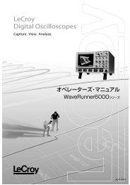
Using LeCroy's Eye Doctor to De-Embed Probes - Teledyne LeCroy

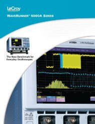
A P P L I C A T I O N B R I E F
Using LeCroy’s Eye Doctor to De-Embed Probes
(LAB_WM772)
Eye Doctor is a software tool that
operates inside of LeCroy oscilloscopes.
The tool consists of two major
features:
Virtual Probing
Ideal Equalizer Emulation
The Virtual Probing feature, which is
the focus of this application brief,
enables a variety of advantages in
signal probing situations including:
1. The ability to compensate for
probe loading effects by allowing
you to see waveforms that occur in a
circuit as they would with and without
the probe connected to it.
2. The ability to acquire waveforms
that occur in locations other than the
probing point.
This is an initial investigation into
compensating for probe loading use
the D11000PS/D13000PS Differential
Probe System and the
SDA11000 Serial Data Analyzer.
This application brief assumes that
you are familiar with the basics of
LeCroy’s Eye Doctor software as
described in the operator’s manual
available on LeCroy’s Website at:
http://www.lecroy.com
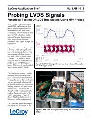
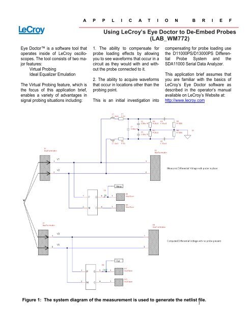
Figure 1: The system diagram of the measurement is used to generate the netlist file.
1

The schematic used to generate the
netlist file is shown in Figure 1. The
upper circuit represents the probe
impedance placed on a perfectly
matched differential pair. The scope
is measuring the differential component
of the signal. The mode conversion
blocks are used to provide a
differential signal that represents the
signal measured by the scope.
The lower circuit is simply the same
ideal differential pair of signals with
no probe impedance present. The
filter calculated using this schematic
will transform the signal acquired by
the scope (Meas) to that with no
probe (Out).
The resulting netlist is shown as the
text file in Figure 2, with the manually
added stimulation lines shown in
bold.
The netlist shown in this file was
compiled and filter response of the
loading correction filter was plotted,
using a third party math program, as
a check to make sure that the results
were as expected. The correction
filter response plot is shown in
Figure 3.
Based on measurement and simulation
of the actual probe tip loading
loss and loss of the loading equivalent
circuit this looks exactly as it
should. This step is not required but
it was included as an assurance
check.
Figure 2: The netlist corresponding to the system diagram
in Figure 1
2
Figure 3: Frequency response of the loading correction
filter

At this point the SDA 11000 scope
and D13000PS probe were set up to
acquire a pseudo-random bit sequnce
(PRBS) test signal. The result
of that signal acquisition is
shown in Figure 4.
Figure 4: The PRBS signal as measured using the D13000PS
probe and SDA11000.
The next step is to setup a math
function using the Eye Doctor Virtual
Probe Math function as shown in
Figure 5. Note that the text file,
“diff_probe_comp_1.txt”, containing
the netlist is entered into the System
Description field. The settings for
the other fields are to be found in the
Eye Doctor operator’s manual
Figure 5: The setup for the Virtual Probe math function.
3

The output of the Virtual Probe function
shows the waveform as it would
be seen if the probe was not present
to load the signal. Figure 6 shows
the acquired trace overlaid by the
output of the virtual probe. Note that
the ‘unloaded’ trace shows slightly
higher peak values immediately after
each state transition. The effects
are minimal because the scope’s 11
GHz bandwidth is less than that of
the probe.
Figure 6: A comparison of the “loaded” (trace Z1) and
“unloaded” (trace Z2) responses of a 13 GHz probe using an 11
GHz Scope
Figure 7 shows a similar measurement
using an 11 GHz, D11000
probe on an SDA13000 which has a
bandwidth of 13 GHz. The probe
loading effects are more pronounced
in this example.
In these examples we have shown
how LeCroy’s Eye Doctor Virtual
Probing feature can be used to deembed
probe loading effects from
your measurement data. This capability
greatly enhances the usability
of the scope in signal integrity
measurements by improving accuracy.
Figure 7: A comparison of the “loaded” (trace F1) and
“unloaded” (trace F2) responses of an 11 GHz probe using a 13
GHz Scope
4