I. What is MATLAB? II. Launching MATLAB
I. What is MATLAB? II. Launching MATLAB
I. What is MATLAB? II. Launching MATLAB

You also want an ePaper? Increase the reach of your titles
YUMPU automatically turns print PDFs into web optimized ePapers that Google loves.
<strong>MATLAB</strong> Tutorial<br />
Mark Goldman, Wellesley College<br />
Th<strong>is</strong> tutorial <strong>is</strong> intended to get you acquainted with the <strong>MATLAB</strong> programming<br />
environment. It <strong>is</strong> not intended as a thorough introduction to the program, but rather as a<br />
practical guide to the most useful functions and operations to be used in th<strong>is</strong> course. For<br />
additional references and to see a l<strong>is</strong>t of some of the many wonderful people who generously<br />
contributed to th<strong>is</strong> tutorial, see “Acknowledgments and References” at the end of th<strong>is</strong> document.<br />
I. <strong>What</strong> <strong>is</strong> <strong>MATLAB</strong>?<br />
<strong>MATLAB</strong> <strong>is</strong> a programming environment for working with numerical data and, to a lesser<br />
extent, symbolic equations. <strong>MATLAB</strong> uses an interpreted language, which means the code <strong>is</strong><br />
compiled (translated from what you type into machine-readable code) and run as you type it in.<br />
For th<strong>is</strong> reason, it <strong>is</strong> an easy environment in which to perform a few manipulations on some data<br />
and plot the output without having to include a lot of the basic declarations required by more<br />
traditional programming languages. In addition, <strong>MATLAB</strong> contains a vast array of built-in<br />
functions for performing manipulations on data.<br />
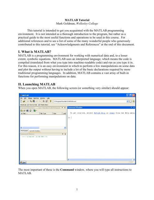
<strong>II</strong>. <strong>Launching</strong> <strong>MATLAB</strong><br />
When you open <strong>MATLAB</strong>, the following screen (or something very similar) should appear:<br />
The most important of these <strong>is</strong> the Command window, where you will type all instructions to<br />
<strong>MATLAB</strong>.<br />
1
The Workspace window l<strong>is</strong>ts all variables and their sizes and class (array, string, etc.). Th<strong>is</strong><br />
window can be useful in debugging (i.e. finding the errors in) your code.<br />
The Command H<strong>is</strong>tory window tells you the most recent commands. You can double-click on<br />
a previous command to run it again (to save you re-typing).<br />
You can open or close these windows by choosing the items from the Desktop menu.<br />
The Current Directory <strong>is</strong> d<strong>is</strong>played in the long horizontal box along the top toolbar of the<br />
program. Th<strong>is</strong> <strong>is</strong> the default directory that <strong>MATLAB</strong> uses when you save your work or open<br />
files. You should set th<strong>is</strong> to the directory (e.g. the Desktop or a folder) in which you plan to<br />
locate your work. You can set th<strong>is</strong> directory by clicking the “...” button to the right of the<br />
Current Directory box and choosing an appropriate location. Th<strong>is</strong> information can alternatively<br />
be set using the Current Directory window that appears as a tab in the same space as the<br />
Workspace window.<br />
<strong>II</strong>I. Using <strong>MATLAB</strong> as your calculator<br />
At the most basic level, <strong>MATLAB</strong> can be used as your calculator with +, −, *, and / representing<br />
addition, subtraction, multiplication, and div<strong>is</strong>ion respectively.<br />
Let’s play a bit with th<strong>is</strong> (type along when you see the prompt “>>”):<br />
>> 2+2<br />
ans =<br />
4<br />
>> (2*(1+5))/3<br />
ans =<br />
4<br />
“ans=” <strong>is</strong> <strong>MATLAB</strong> shorthand for “the answer <strong>is</strong>…”. If you are not sure about the order of<br />
operations, it <strong>is</strong> always safe to be explicit by using extra parentheses!<br />
There are also very many built-in functions, e.g.<br />
>> sin(pi/2)<br />
ans =<br />
1<br />
Note that “pi=3.14159…” <strong>is</strong> known by <strong>MATLAB</strong> and that <strong>MATLAB</strong> <strong>is</strong> case-sensitive (try<br />
typing Sin(pi/2) and see what happens).<br />
2
IV. Assigning variables<br />
A variable <strong>is</strong> a storage space in a computer for numbers or characters. The equal sign “=” <strong>is</strong><br />
used to assign a numerical value to a variable:<br />
At the command prompt, type:<br />
>> a = 5<br />
You've just created a variable named a and assigned it a value of 5. If you now type<br />
>> a*5<br />
you get the answer 25.<br />
Now type<br />
>> b = a*5;<br />
You've just made a new variable b, and assigned it a value equal to the product of the value of a<br />
and 5. By adding a semicolon, you've supressed the output from being printed. Supressing the<br />
output will be important later. To retrieve the value of b, just type<br />
>> b<br />
without a semicolon.<br />
Now try typing<br />
>> a = a + 10<br />
Th<strong>is</strong> re-assigns to the variable a the sum of the previous value of a (which was 5), plus 10,<br />
resulting in the new value of the variable a being 15. Note: th<strong>is</strong> illustrates that ‘=’ means<br />
‘assign’ in <strong>MATLAB</strong>. It <strong>is</strong> not a declaration that the expressions on the two sides of the ‘=’ sign<br />
are ‘equal’ (because certainly a cannot equal itself plus 10!). We will see later that a double<br />
equal sign “==” <strong>is</strong> used when we want to test if two quantities are equal to each other.<br />
V. Vectors and Matrices<br />
In <strong>MATLAB</strong>, all numerical variables are real-valued matrices, or arrays (of type "double" for<br />
the programmers out there). Th<strong>is</strong> makes it easy to perform manipulations on groups of related<br />
numbers at the same time. You did not realize it, but the variables you created above are 1 row<br />
by 1 column (or “1x1” for short) matrices. To confirm th<strong>is</strong>, click in the Workspace panel to<br />
make it active, then in the main <strong>MATLAB</strong> menus choose View>>Choose Columns>>Size to<br />
see that the variables you created above such as a and b are actually 1 x 1 arrays.<br />
Let's see how more about how arrays work. Type<br />
>> a = [1 2 3 4 5]<br />
3
a =<br />
1 2 3 4 5<br />
You have just created an array containing the numbers 1 through 5. Th<strong>is</strong> array can be thought of<br />
as a matrix that <strong>is</strong> 1 row deep and 5 columns wide (often called a row vector). To confirm th<strong>is</strong>,<br />
use the size command which tells you the number of rows (first element returned) and number<br />
of columns (second element returned) in an array:<br />
>> size(a)<br />
ans =<br />
1 5<br />
To obtain the number of elements in a vector, use the length command:<br />
>> length(a)<br />
ans =<br />
5<br />
You can also add or multiply arrays by a constant, or add arrays. Try:<br />
>> b = 2*a<br />
b =<br />
>> b+a<br />
ans =<br />
2 4 6 8 10<br />
3 6 9 12 15<br />
You can access the value of a given element of a or b by using parentheses. Type<br />
>> a(3)<br />
>> b(4)<br />
and you see the values of the 3 rd element of the a array and the 4 th element of the b array,<br />
respectively. You can also use b(end) or a(end) to see the last element.<br />
Finally, you can append one vector onto another to make a longer vector. For example, try<br />
typing:<br />
>> a = [a 8 9 10]<br />
a =<br />
1 2 3 4 5 8 9 10<br />
4
Th<strong>is</strong> re-assigns the variable a to equal a new row vector containing the elements of the previous<br />
vector a, followed by the new elements [8 9 10].<br />
---------------<br />
If you prefer to arrange your array into a column (i.e. a 5 row x 1 column matrix, or column<br />
vector), you can do th<strong>is</strong> by separating the elements by semicolons:<br />
>> a = [1; 2; 3; 4; 5]<br />
a =<br />
1<br />
2<br />
3<br />
4<br />
5<br />
>> size(a)<br />
ans =<br />
5 1<br />
Now suppose we decide that we really would have liked to organize the elements of a into a row<br />
vector. There are two ways to get back to our original assignment (well… 3 ways if you include<br />
just re-typing, but we’re far too smart to do that!):<br />
Method 1: use the uparrow key (↑) to scroll back through your previous commands until you<br />
reach the a = [1 2 3 4 5] command and then press return (equivalently, you also could have used<br />
the Command H<strong>is</strong>tory window). The downarrow key (↓) scrolls forward through previous<br />
commands (in case you scroll back too far).<br />
For practice, undo th<strong>is</strong> by double-clicking on a = [1; 2; 3; 4; 5] in the Command H<strong>is</strong>tory window<br />
so that a <strong>is</strong> again a column vector.<br />
Method 2: Another way to change from a row to a column vector <strong>is</strong> to do the transpose<br />
operation, denoted by a single quotation mark ′. The transpose of a matrix exchanges the rows<br />
and columns of a matrix.<br />
Let’s try it:<br />
>> a = a'<br />
a =<br />
1 2 3 4 5<br />
The above line re-assigns to the variable a the values of the row vector a'.<br />
---------------<br />
5
Now let’s construct (i.e. create and assign values to) a matrix that we will name “m”:<br />
>> m = [1 2; 3 4]<br />
m =<br />
1 2<br />
3 4<br />
Note the syntax: elements in the same row are separated by spaces. A new row <strong>is</strong> designated by<br />
the semicolon.<br />
To find out the value of the element in the 2 nd row, 1 st column of m, type:<br />
>> m(2,1)<br />
ans =<br />
3<br />
Similarly, if we would like to re-assign th<strong>is</strong> element to equal 7 instead of 3 we would type:<br />
>> m(2,1) = 7<br />
m =<br />
1 2<br />
7 4<br />
The transpose of matrix m <strong>is</strong> found by typing:<br />
>> m'<br />
ans =<br />
1 7<br />
2 4<br />
Notice that the previous 1 st row <strong>is</strong> now the first column and the previous 2 nd row <strong>is</strong> now the<br />
second column.<br />
VI. More on Vectors, plus Plotting a Graph<br />
Suppose we want to plot a graph of the function y = x^2 from x = 0 to x=5 with points drawn<br />
every 0.5 units along the x-ax<strong>is</strong> (note: ^ <strong>is</strong> <strong>MATLAB</strong>’s symbol for ra<strong>is</strong>ing a number to a power).<br />
We could specify the x vector explicitly, writing x = [0 0.5 1.0 1.5 etc.] but th<strong>is</strong> would be quite<br />
painful, especially if x were a larger vector.<br />
Instead <strong>MATLAB</strong> uses the colon operator (:) to specify regular sequences of elements. Try<br />
typing<br />
>> 1:5<br />
6
ans =<br />
1 2 3 4 5<br />
We can also increment (or decrement) by an amount other than one by typing, for example:<br />
>> 10:-2:4<br />
ans =<br />
10 8 6 4<br />
In general, the syntax for creating arrays in th<strong>is</strong> manner <strong>is</strong> start number:size of step:end number.<br />
Now let’s go on to our plotting y=x^2 example. We assign x as:<br />
>> x = 0:0.5:5<br />
To obtain the squares of the elements of x, one might think we should type x^2 or x*x but either of<br />
these (which are equivalent) attempts to multiply two row vectors by each other using the rules<br />
of matrix multiplication and th<strong>is</strong> <strong>is</strong> not a legal mathematical operation:<br />
>> x*x<br />
??? Error using ==> mtimes<br />
Inner matrix dimensions must agree.<br />
In matrix multiplication, the number of columns of the first matrix must equal the number of<br />
rows of the second matrix, e.g. (1:3)*(1:3) gives a syntax error but (1:3)*(1:3)' would be ok and<br />
gives 14 (try it! Remember that you can use the up arrow to go back to a previous line and rev<strong>is</strong>e<br />
it). The reason <strong>MATLAB</strong> says “Inner matrix dimensions must agree” <strong>is</strong> because we can<br />
only multiply a M 1 x N 1 element matrix by a M 2 x N 2 if N 1 = M 2 , i.e. if the inner two of the 4<br />
l<strong>is</strong>ted matrix dimensions agree (i.e. are equal). Note that the resulting matrix has size M 1 x N 2 by<br />
the rules of matrix multiplication. Thus, a 1 x 3 matrix can’t be multiplied by another 1 x 3<br />
matrix but it can be multiplied by the transpose of a 1 x 3 matrix (which has dimensions 3 x 1).<br />
If matrix multiplication <strong>is</strong> unfamiliar to you, please let me know and we can go over it. If you<br />
are just rusty, I recommend brushing up on it.<br />
So how do we take the square of each element of a matrix? To multiply two arrays by each other<br />
element by element, you have to add a period before the operator. For example, the following<br />
two statements both make a vector y whose elements contain the squares of the elements of x:<br />
>> y = x.*x<br />
>> y = x.^2<br />
Th<strong>is</strong> <strong>is</strong> a general <strong>MATLAB</strong> syntax: always add the . before any operation that you would like to<br />
conduct element by element (e.g. addition, subtraction, div<strong>is</strong>ion, etc.).<br />
---------------<br />
7
Great! Now we’re ready to plot y vs. x using the plot command. To do th<strong>is</strong>, type:<br />
>> figure(1)<br />
>> plot(x,y)<br />
Th<strong>is</strong> brings up a window entitled “Figure No. 1” and plots x on the horizontal ax<strong>is</strong> and y on the<br />
vertical ax<strong>is</strong>. All figures are numbered in <strong>MATLAB</strong>--you can use any integer you want, and if<br />
you just type 'figure' it will make up a number for you (specifically, the smallest unused<br />
positive integer). If you are only plotting a single figure, you can omit the figure command and<br />
<strong>MATLAB</strong> will automatically draw your plot in Figure No. 1.<br />
If you want to print the figure, you can do that by choosing File>>Print from within the Figure<br />
window. I recommend using File>>Page Setup to make sure the window maps onto the paper<br />
you're using in a pretty way.<br />
Now let's tackle the only slightly more challenging problem of plotting more than one function at<br />
a time. Type:<br />
>> hold on<br />
>> plot(x,x,'r')<br />
The hold on command tells <strong>MATLAB</strong> to hold onto what <strong>is</strong> currently on the plot if new data <strong>is</strong><br />
plotted; otherw<strong>is</strong>e, the default behavior <strong>is</strong> to replace what <strong>is</strong> there (you can go back to th<strong>is</strong> by<br />
typing 'hold off'). The second function simply plots x versus itself in red. The last argument to<br />
the plot function (i.e. item you specify, in th<strong>is</strong> case 'r') <strong>is</strong> a string (i.e. array of characters)<br />
where you can pass some parameters to the plotting function. The single quotes <strong>is</strong> the syntax for<br />
telling <strong>MATLAB</strong> that the r <strong>is</strong> the character r and not a variable you may have created and named<br />
r. To really get into all of the various options <strong>is</strong> complicated (type 'help plot' if you want to<br />
see), but if you follow the pattern of the examples here you might not need to get into all of the<br />
details.<br />
Now we have two plots in the same window. These plots are lines through the points we have<br />
given <strong>MATLAB</strong>. Suppose we want to show the data points. We can do th<strong>is</strong> by adding two new<br />
plots. First, close the previous figure window by using close(#), where # <strong>is</strong> the figure number,<br />
or by clicking the close box on the window itself. Then type:<br />
>> plot(x,y,'o')<br />
>> plot(x,x,'ro')<br />
Th<strong>is</strong> adds two new plots. The first plots y vs. x using o's at each point. The second plots x vs. x<br />
using o's at each point and the color red.<br />
Now let's add some labels to the graph and practice changing the ax<strong>is</strong> limits using the title,<br />
xlabel, ylabel, legend, and ax<strong>is</strong> commands. Type:<br />
8
title('First two powers of the integers and half integers')<br />
>> xlabel('Integers and half integers')<br />
>> ylabel('First two powers')<br />
>> legend('second power','first power')<br />
>> ax<strong>is</strong>([0 6 0 50])<br />
If you would like more help on the syntax of any of these commands, type ‘help commandname’.<br />
In th<strong>is</strong> course, you will often be interested in putting more than one plot in a window for clarity<br />
and to save paper. Th<strong>is</strong> <strong>is</strong> where the subplot command comes in. Close the window you have<br />
been working in and now type:<br />
>> figure(1)<br />
>> subplot(2,1,1)<br />
>> plot(x,y,'o')<br />
>> title('Integers and half integers squared')<br />
>> subplot(2,1,2)<br />
>> plot(x,x,'o')<br />
>> title('Integers and half integers')<br />
subplot allows you to define an MxN matrix of plotting panels within a figure, where M=the<br />
number of rows of plotting panels within the figure <strong>is</strong> the first argument of the function, N=the<br />
number of columns of plotting panels <strong>is</strong> the second argument, and the third argument describes<br />
which plotting panel to draw in presently. Above, we have defined a 2x1 matrix of plotting<br />
panels, and plotted x vs. y in the 1 st one and x vs. x in the 2 nd one. Note that we specify the title<br />
after calling the subplot and plot commands.<br />
V<strong>II</strong>. Functions<br />
<strong>MATLAB</strong> has many built-in functions that allow many operations to be carried out in a single<br />
line. You just learned about a few (e.g. size(matrix) and plot(vector1,vector2,formatting)).<br />
The general format <strong>is</strong> functionname(arguments) with the appropriate function name and<br />
arguments. For example, in the course we will often create an array t of time points:<br />
>> t=1:0.25:6;<br />
Then,<br />
>> x=sin(t)<br />
creates a vector of the same size as t, with values of the sine of t at each point. (try plotting<br />
x=sin(t) vs. t to check th<strong>is</strong> out).<br />
Here’s another useful one:<br />
>> y=zeros(1,5)<br />
9
The zeros function assigns to the variable y a 1 x 5 array of zeros.<br />
V<strong>II</strong>I. Logical structures: loops, the if statement, and logical operators<br />
A) For loops<br />
Now that you can perform simple operations, let’s learn how to group operations together using<br />
computer logic. The first structure that will be useful <strong>is</strong> known as the “for loop”. The for<br />
command <strong>is</strong> useful when we would like to perform the same operation or set of commands many<br />
times. For example, suppose we wanted to know the square of the numbers 1, 4, and 5. We<br />
could type 1^2, followed by 4^2, followed by 5^2, but th<strong>is</strong> would clearly be quite tedious<br />
(especially if we wanted to know the square of far more numbers). A for loop <strong>is</strong> perfect for th<strong>is</strong><br />
type of situation because we are performing the same operation (squaring a number) over and<br />
over again. The syntax for accompl<strong>is</strong>hing th<strong>is</strong> <strong>is</strong> the following. Type:<br />
>> for A=[1 4 5]<br />
d<strong>is</strong>p(‘You will see the current value of A^2 below:’)<br />
A^2<br />
end<br />
The output you should see in response to th<strong>is</strong> <strong>is</strong>:<br />
You will see the current value of A^2 below:<br />
ans =<br />
1<br />
You will see the current value of A^2 below:<br />
ans =<br />
16<br />
You will see the current value of A^2 below:<br />
ans =<br />
25<br />
Notice what happened: <strong>MATLAB</strong> ran the two lines “d<strong>is</strong>p(‘You will…’)” and “A^2” three<br />
separate times, once for each of the elements in the vector [1 4 5]. Note that the d<strong>is</strong>p command<br />
prints to the screen whatever its argument <strong>is</strong> (in th<strong>is</strong> case, a string of text). The above example<br />
also illustrates the syntax of a for loop, namely the first line of a for loop <strong>is</strong> “for variable =<br />
vector”, the last line <strong>is</strong> “end”, and the in-between lines are the commands to be executed over<br />
and over again, once for each element of the vector. Specifically, what the for loop does <strong>is</strong>:<br />
10
1. Assign the variable (e.g. A) to equal the first element of vector (e.g. 1 if the vector <strong>is</strong><br />
[1 4 5]).<br />
2. Execute all lines following the “for variable = vector” line and before the “end” line.<br />
3. “Loop” back to the beginning, now assigning variable (e.g. A) to equal the 2 nd element<br />
of vector (e.g. 4 in the example above), and again execute all lines before the “end” line.<br />
4. Keep looping through the elements of vector until all values have been used. When the<br />
last element of vector (e.g. 5 in the example above) has been assigned to variable and the lines<br />
before the “end” line have been executed, the loop <strong>is</strong> fin<strong>is</strong>hed executing.<br />
We can also use for loops to assign values to the elements of a matrix. If we want to make a<br />
vector y containing the values of sin(x) from x=0 to x=pi in steps of pi/10, we could type:<br />
>> clear y<br />
>> x=0:pi/10:pi<br />
>> for i=1:length(x)<br />
y(i) = sin(x(i))<br />
end<br />
Th<strong>is</strong> program has the same effect as typing y = sin(x), but illustrates how for loops work. It first<br />
clears the previous value of y from memory with the command clear y. It then creates the<br />
vector x. Then, it cycles through the loop once for each value of the array 1:length(x) (which<br />
has values 1 through 11 since the length of the vector x <strong>is</strong> 11) and, for each value of i, it assigns<br />
to the i th element of array y, the sine of the i th element of array x (e.g. y(1) = sin(x(1)) = sin(0) = 0<br />
because the first element of array x <strong>is</strong> x(1)=0.) Check th<strong>is</strong> by typing:<br />
>> y(1)<br />
Note: the above code typically runs much slower than if we were to use the vector assignment<br />
operations we’ve learned so far (like y=sin(x)). For th<strong>is</strong> reason, using vector operations <strong>is</strong><br />
preferable to using for loops when possible. However, the above <strong>is</strong> a nice example of the use of<br />
the for loop and <strong>is</strong> similar to the types of for loops we will use next week so make sure you<br />
understand it.<br />
B) If statement<br />
The other most useful logical operation <strong>is</strong> the “if” statement. Try:<br />
>> for A=1:5<br />
if (A > 3)<br />
A<br />
end %end of if statement<br />
end %end of for loop<br />
Th<strong>is</strong> program steps through the values in the array 1:5 and, if the value of A during the current<br />
step <strong>is</strong> greater than 3, prints th<strong>is</strong> value of A. Note that for loops and if statements always need to<br />
be concluded with an end statement. Also note the %: anything following the % sign <strong>is</strong> a<br />
comment (i.e. note to yourself) and <strong>is</strong> ignored by <strong>MATLAB</strong>. Commenting your code <strong>is</strong><br />
tremendously useful, as it allows you to remember the logic of your code when you look back<br />
11
at it. It also <strong>is</strong> easier for others (e.g. your grader…) to follow your logic. You should use<br />
comments liberally.<br />
C) Boolean (true or false) logic<br />
Often we simply want to know if something <strong>is</strong> true or false. <strong>MATLAB</strong> denotes true by the<br />
integer 1 and false by the integer 0. For example, try:<br />
>> a=1:6;<br />
>> b = (a>2)<br />
The above line assigns to b a vector of the same size as a with 0’s (false’s) and 1’s (true’s)<br />
designating whether that element of a was greater than 2. You can also do < (less than), = (greater than or equal to), == (equal to; note that we use the double equal<br />
sign for the logical operation of comparing two values. The single equal sign <strong>is</strong> only used for<br />
assigning values to variables. See the example in the next section).<br />
D) While loop<br />
Another type of loop, similar to the for loop, <strong>is</strong> called the while loop. If you are interested, you<br />
can get more information about th<strong>is</strong> by typing ‘help while’ at the command prompt or by<br />
consulting the Pratap book.<br />
IX. More logic, and M files<br />
Up until now, you've typed all of your commands directly into the command line. Of course, for<br />
doing your homework, you'll probably want to put your code into a file so you can print it out<br />
easily and remember what you have done. Let's make an “m-file” for the last example.<br />
In the <strong>MATLAB</strong> command window, choose File>>New...M-file from the File menu. Now you<br />
should have an open text window. Re-type the following lines into the file:<br />
for A=1:5<br />
if (A > 3)<br />
A<br />
end %end of if statement<br />
end %end of for loop<br />
Now choose File>>Save. Save it to the Desktop (or make a folder for yourself on the desktop<br />
and save it there) as 'Lab1a.m' or something like that, where the “.m” at the end of the filename<br />
tells <strong>MATLAB</strong> that th<strong>is</strong> <strong>is</strong> a <strong>MATLAB</strong> program. Note: do not use spaces or special characters<br />
in file names (the underscore character ‘_’ <strong>is</strong> sometimes helpful in place of a space). Now,<br />
before running your m-file, make sure you are working in the same directory as your file by<br />
checking the Current Directory in the toolbar. If the Current Directory <strong>is</strong> not set to the directory<br />
where your file <strong>is</strong>, change it now.<br />
12
Now you are ready to run your M-file. Type ‘Lab1a’ and the commands should run. If you ever<br />
want to run an m-file without being in that directory, see 'help addpath'. Alternatively, you can<br />
both save what you have typed and run your code simultaneously by clicking the button in<br />
the toolbar which <strong>is</strong> equivalent to Debug>>Run (or Save and Run) or the F5 key.<br />
Let’s add a bit more logic to our loop. Rev<strong>is</strong>e your m-file to read:<br />
clear s; %clears the variable s out of memory<br />
for A=1:5<br />
if (A > 3)<br />
A %print out the value of A<br />
elseif (A==3) %note syntax: “A equals 3” <strong>is</strong> denoted by a double equal sign!<br />
%the single “=” <strong>is</strong> used only for assigning values to variables.<br />
%Confusing these <strong>is</strong> one of the easiest ways to have an error in your code!<br />
s = ‘hello’ %to print and/or assign a text string, put it inside single quotation marks<br />
else %A equals 1 or 2<br />
-A %print out negative of the value of A<br />
end %end of if statement<br />
end<br />
%end of for loop<br />
Can you predict what th<strong>is</strong> will output? Try it out by saving th<strong>is</strong> file (always make sure to<br />
remember to save before running your code—th<strong>is</strong> <strong>is</strong> a common error!) and running it. The<br />
if…elseif…else structure <strong>is</strong> great for going through logic. The elseif or else can be omitted if not<br />
needed. Type ‘help if’ for more information.<br />
The ‘clear s’ statement at the beginning of th<strong>is</strong> script removes any information that might have<br />
been in the variable s from the computer’s memory (e.g. if you had previously assigned a<br />
variable s earlier in your <strong>MATLAB</strong> session). You should always clear all variables from the<br />
computer’s memory before starting a new program. Usually, it <strong>is</strong> simplest to just type ‘clear all’<br />
which removes all variables from memory. To close all open windows (so that you don’t end up<br />
with plots from old runs appearing in your new figures), type ‘close all’.<br />
X. Getting help<br />
There are many places to get help for <strong>MATLAB</strong>. Some of them are:<br />
1. Typing ‘help commandname’ where commandname designates the command you<br />
want to know the syntax of.<br />
Alternatively (I prefer th<strong>is</strong> one), type ‘doc commandname’ which brings up the much<br />
prettier <strong>MATLAB</strong> help window.<br />
2. If you do not know the command name, you can type ‘lookfor<br />
ARelatedWordYouCanThinkOf’. For example, if you wanted to know about sinusoidal functions,<br />
you could type ‘lookfor sine’. If you get sick of its scrolling through zillions of functions that<br />
use sinusoidal functions, you can type CTRL-C to interrupt a command and get back to the<br />
command prompt.<br />
3. You can also use <strong>MATLAB</strong>’s help/search engine by clicking on “Help>><strong>MATLAB</strong><br />
Help” in the main <strong>MATLAB</strong> window. Type words you are looking for into the “Search” box<br />
13
(in the left pane of th<strong>is</strong> window) or you can try to look through “Contents”. In my experience,<br />
“Search” <strong>is</strong> much better than the lookfor command.<br />
4. Websites:<br />
<strong>MATLAB</strong>’s webpage:<br />
http://www.mathworks.com/access/helpdesk/help/techdoc/matlab.shtml<br />
Quick reference for many <strong>MATLAB</strong> commands<br />
http://web.usna.navy.mil/%7Emecheng/DESIGN/CAD/<strong>MATLAB</strong>/matlab/matlab.<br />
html<br />
Zillions of other <strong>MATLAB</strong> tutorials:<br />
http://www.google.com/search?q=matlab+tutorials&ie=UTF-8&oe=UTF-8<br />
Books:<br />
▪ Simple accessible intro: Pratap, R. Getting Started with <strong>MATLAB</strong> 7: A Quick<br />
Introduction for Scient<strong>is</strong>ts and Engineers (Oxford University Press, 2006).<br />
▪ More advanced and thorough: Hanselman, D. and Littlefield, B. Mastering<br />
<strong>MATLAB</strong> 6 (Prentice Hall, 2001).<br />
5. When all else fails, type ‘why’ at the command prompt as many times as <strong>is</strong> necessary<br />
(type ‘help why’ for an explanation).<br />
Acknowledgments<br />
Thanks to the following people who generously contributed material to th<strong>is</strong> tutorial:<br />
Yue Hu (Wellesley Physics)<br />
Stephen van Hooser & Larry Abbott (Brande<strong>is</strong> University)<br />
Justin Werfel (M.I.T.)<br />
Mark Nelson (Univ. of Illino<strong>is</strong>)<br />
14
Exerc<strong>is</strong>es to do in lab, time allowing, or at home (do these all in separate .m files)<br />
These exerc<strong>is</strong>es should both serve as a math review and get you some more practice using<br />
<strong>MATLAB</strong>. Feel free to consult the solutions (next page) as needed, especially if you are new to<br />
programming--it <strong>is</strong> most important for you to be able to understand how the code in the solutions<br />
works.<br />
1. Nested for loops<br />
It <strong>is</strong> common in programming that we want to repeat over and over again a set of code that has a<br />
for loop in it. To do th<strong>is</strong> we make a second for loop inside of which the first for loop sits. We call<br />
the first for loop the “outer loop” because its for and end statements contain the second, “inner”<br />
for loop.<br />
Predict what the output of the code below will produce by working through it with pencil<br />
and paper (i.e. try to predict what the computer will output to the screen; in doing th<strong>is</strong>, you may<br />
also find it useful to calculate the values of NumTimesThroughOuterLoop and<br />
NumTimesThroughInnerLoop that <strong>MATLAB</strong> calculates as the program runs but that aren’t printed<br />
to the screen because of the semicolon). After doing th<strong>is</strong>, create an m-file and type in the code<br />
below to check your answers.<br />
NumTimesThroughOuterLoop = 0; %th<strong>is</strong> variable will keep track of the number<br />
%of times the code has run through the outer loop<br />
NumTimesThroughInnerLoop = 0; %th<strong>is</strong> variable will keep track of the number of times<br />
%the code has run through the inner loop<br />
for i=10:10:30<br />
NumTimesThroughOuterLoop = NumTimesThroughOuterLoop + 1;<br />
for j=1:2<br />
NumTimesThroughInnerLoop = NumTimesThroughInnerLoop + 1;<br />
i_plus_j = i + j<br />
end<br />
end<br />
NumTimesThroughOuterLoop<br />
NumTimesThroughInnerLoop<br />
2. Multiplying a vector by a matrix<br />
Multiply the column vector v=[1; 2] by the matrix A=[2 3; 3 4; 4 5]<br />
i) First, do th<strong>is</strong> matrix multiplication out ‘by hand’ as a review of matrix math (if you can’t<br />
remember the formula, it’s l<strong>is</strong>ted in part (iii), or see Dayan & Abbott Appendix A.1).<br />
ii) Next, do it the easy way by using <strong>MATLAB</strong>’s built-in commands. Do th<strong>is</strong> in the command<br />
line (i.e. not in an m-file; for the homework, you do not need to turn in anything for th<strong>is</strong>).<br />
iii) Finally, pretend <strong>MATLAB</strong> didn’t have built-in commands for doing matrix multiplication.<br />
Instead, write an m-file that implements the matrix multiplication rule:<br />
N<br />
w( i) = ! A( i, j)* v( j)<br />
j=<br />
1<br />
where the vector and matrix elements above are written in <strong>MATLAB</strong> notation, so that w(i) <strong>is</strong> the<br />
i th element of w and A(i,j) <strong>is</strong> the element located in the i th row and j th column of the matrix A.<br />
15
Also by the rules of matrix multiplication, note that N = the number of rows of v = number of<br />
columns of A (in our case, N=2). Put your final answer in the vector w.<br />
Before programming th<strong>is</strong>, confirm that the formula above corresponds to how you<br />
determined the elements w(i), i=1, 2, and 3, when you multiplied out the matrix by hand.<br />
Then, to program th<strong>is</strong>, you will first want to type the command “clear all” which will<br />
make sure all variables have been cleared. You will then want to assign v and A to the given<br />
values above and initialize w to be an appropriately dimensioned matrix of zeros before doing<br />
the sum (i.e. assign w an initial set of values at the start of your code. Th<strong>is</strong> tells <strong>MATLAB</strong> to set<br />
up a placeholder for the w vector so that it’s ready to assign values to w when you do your future<br />
calculations. Although initialization <strong>is</strong> not required, doing th<strong>is</strong> makes <strong>MATLAB</strong> code run much<br />
faster so it’s a good habit to initialize all unknown matrices to some value such as zero at the<br />
beginning of your code).<br />
Finally, use 2 nested for loops. Note that at the conclusion of th<strong>is</strong> program, we would like<br />
to have assigned values to w(i) for each of its 3 elements, i.e. for i=1, i=2, and i=3. Thus, the<br />
outer loop will be over the values of the index i.<br />
To determine any individual value w(i), we can build up its final value one step at a time.<br />
First, we initialize w(i) to equal zero (which you did above). Then, we add successive terms in<br />
the sum above to it (just as you did when you did the matrix multiplication by hand). That <strong>is</strong>, we<br />
need to keep repeating the operation “add to the current value of w(i) an additional amount<br />
A(i,j)*v(j)” for each term in the sum above (i.e. for j=1 and j=2 in our case). More generally, if<br />
we were multiplying bigger matrices and vectors, we would need to add terms A(i,j)*v(j) for<br />
each of the N=length(v) elements of v).<br />
Hint: <strong>What</strong> line of code in <strong>MATLAB</strong> increases w(i) by an amount A(i,j)*v(j), i.e. assigns<br />
to w(i) its previous value plus an amount A(i,j)*v(j)?<br />
3. Numerical calculation of derivatives<br />
Taking derivatives <strong>is</strong> easy with <strong>MATLAB</strong> if we use some clever functions.<br />
Recall that the derivative of the function x(t) at time t <strong>is</strong> defined as:<br />
dx( t) x( t + ! t) # x( t)<br />
= lim<br />
dt ! t"<br />
0 ! t<br />
Numerically, we can approximate the derivative by using a very small (although not strictly zero<br />
because the computer can’t divide by zero) value of Δt th<strong>is</strong> operation <strong>is</strong> very easy to do:<br />
i) We define a vector t=t_start:dt:t_end that <strong>is</strong> d<strong>is</strong>cretized into steps of size dt (dt <strong>is</strong> really<br />
supposed to be the limit as Δt approaches zero, so we really should say “Δt” for the finite step<br />
sizes we’ll use. However, typing the Δ <strong>is</strong> difficult so we’ll just write ‘dt’. Th<strong>is</strong> <strong>is</strong> the convention<br />
in numerical simulation programs). Assign a variable dt=0.1 and then make a vector t that<br />
goes from t = −1 to t = 1 in steps of size dt. You can do th<strong>is</strong> in the command line.<br />
ii) Then we define the vector x(t). For our example, let’s consider the function x(t) = sin(2*pi*t).<br />
Create th<strong>is</strong> vector in the command line.<br />
Potential point of confusion: Be careful not to confuse the parentheses printed in mathematical<br />
functions (e.g. x(t) meaning “x as a function of t”) and the parentheses used by <strong>MATLAB</strong> when<br />
16
accessing elements of arrays (e.g. x(1) meaning “the first element of the vector x”). For<br />
example, the first element of the t vector, t(1), has value t(1) = −1. Similarly, the first element<br />
of the x vector we just defined <strong>is</strong> x(1) = sin(2*pi*t(1)) = sin(-2*pi) = 0.<br />
For concreteness, check th<strong>is</strong> out by typing x(1) to see what the value of x <strong>is</strong> at the first<br />
time point and x(2) to see what the value of x <strong>is</strong> at the second time point. <strong>What</strong> <strong>is</strong> the value of<br />
x at time t = -0.4 and which element of the array x does th<strong>is</strong> correspond to?<br />
iii) The derivative rule says that to get dx/dt at any time t, we need to take the difference between<br />
x(t+dt) and x(t), and then divide th<strong>is</strong> difference by dt,<br />
e.g. to get the derivative of x at the first time point (t = -1), we would take the difference<br />
between the value of x at the 2 nd time point, x(2) and the value of x at the 1 st time point, x(1), and<br />
then divide th<strong>is</strong> difference by dt:<br />
>> xderiv(1) = (x(2) – x(1))/dt<br />
We would like to know the derivative not just at the first time point but at all time points, e.g. the<br />
derivative of x at the i th time point would be given by:<br />
xderiv(i) = (x(i+1) – x(i))/dt<br />
One can calculate differences between elements of a vector for an entire vector all at once using<br />
the diff command. Type ‘help diff’ and then try entering diff(x) at the command line.<br />
In a .m file, use the diff command to evaluate the derivative of x = sin(2*pi*t) using the t<br />
vector from parts (i) and (ii). Note that diff(x) <strong>is</strong> 1 element shorter than x because there <strong>is</strong><br />
no final element (we can’t take the derivative of the final point because we don’t know the<br />
value of x(t+dt) there). When plotting dx/dt vs. t, therefore plot versus a shorter time<br />
vector that does not include the last element (Hint: to access only the first 3 elements of a<br />
vector b, for example, you would type b(1:3) and to access the 2 nd -to-last element of b you<br />
could type b(end-1) since end corresponds to the index of the last element). Make 2 figures<br />
within the same window, one showing x(t) vs. t and the other dx/dt vs. t.<br />
Compare to the analytic expression for the derivative (i.e. to the exact formula for the<br />
derivative of sin(2πt), which you should calculate). Re-run with dt = 0.01. Can you see<br />
why it helps to have dt very small to calculate accurate derivatives?<br />
17
4. Computing the value of an integral<br />
Recall the definition of an integral as the area under a curve, which can be broken into small<br />
rectangles of size f(x)*Δx around each point x:<br />
b<br />
$<br />
a<br />
f ( x) dx = lim f ( x)<br />
! x<br />
b<br />
#<br />
! x " 0<br />
x = a<br />
That <strong>is</strong>, to integrate a function we want to step through the values of the function. In <strong>MATLAB</strong><br />
notation, we w<strong>is</strong>h to put x into a vector starting at x=a, ending at x=b, and d<strong>is</strong>cretized into steps<br />
of size dx (again, really Δx, but we’ll write ‘dx’ for ease of typing). Thus, in more <strong>MATLAB</strong>-y<br />
notation, we write:<br />
b N N<br />
#<br />
a<br />
" "<br />
f ( x) dx = f ( x( i))* ! x = ! x* f ( x( i))<br />
i= 1 i=<br />
1<br />
3<br />
x 2<br />
dx<br />
1<br />
where N=length(x). Write a simulation which computes ! (and check your answer by<br />
doing th<strong>is</strong> numerically). Try dx=0.1, dx=0.01, and dx=0.001 to test the accuracy of your result.<br />
Hint: Use the command sum to find the sum of the elements of an array.<br />
18
Solutions to Exerc<strong>is</strong>es<br />
1. Nested for loops<br />
i_plus_j = 11<br />
i_plus_j = 12<br />
i_plus_j = 21<br />
i_plus_j = 22<br />
i_plus_j = 31<br />
i_plus_j = 32<br />
NumTimesThroughOuterLoop = 3<br />
NumTimesThroughInnerLoop = 6<br />
2. Multiplying a vector by a matrix<br />
(i)<br />
! 2 3" ! 2*1+<br />
3*2" ! 8 "<br />
# $ ! 1"<br />
# $ # $<br />
3 4 # $ = 3*1 4*2 11<br />
2<br />
+ =<br />
# 4 5$ % & # 4*1+<br />
5*2$ # 14$<br />
% & % & % &<br />
(ii)<br />
>> v = [1; 2]<br />
v =<br />
1<br />
2<br />
>> A = [2 3; 3 4; 4 5]<br />
A =<br />
2 3<br />
3 4<br />
4 5<br />
>> A*v<br />
ans =<br />
8<br />
11<br />
14<br />
(iii) Notice the commenting and how the for loops are formatted for easy readability:<br />
% Lab 1, Exerc<strong>is</strong>e 1, part iii: multiply a vector by a matrix<br />
clear all; %clear all variables from memory<br />
v = [1; 2];<br />
A = [2 3; 3 4; 4 5];<br />
19
% note that because A <strong>is</strong> a 3x2 matrix and v a 2x1 matrix,<br />
% j in the sum should go from 1:2 (2 = length(v))<br />
% and w will be a 3x1 matrix (3=# of rows of A, 1=# of columns of v)<br />
% From the help menu, size(A,1) gives the number of rows of A<br />
w = zeros(3,1); % initialize w to be a matrix of zeros<br />
for i=1:size(A,1) % loop to assign element i of vector w<br />
for j=1:length(v) % loop to perform the sum over j<br />
w(i)=w(i)+A(i,j)*v(j); % add A(i,j)*v(j) to the current value of w(i)<br />
end<br />
end<br />
w %d<strong>is</strong>play w<br />
Note in the code above that you could have simply said “for i=1:3” and “for j=1:2”. The above<br />
code <strong>is</strong> written so that it could more easily be generalized to multiplying matrices and vectors of<br />
different sizes.<br />
3. Numerical derivatives<br />
i)<br />
>> dt = 0.1<br />
>> t = -1:dt:1<br />
ii) x = sin(2*pi*t)<br />
The 7 th element of x <strong>is</strong> x(7) = sin(2*pi*t(7)) = sin(2*pi*(-0.4)) = -0.5878.<br />
iii)<br />
% program to take the derivative of the function sin(t)<br />
% note how the variable names help to make the code clear<br />
clear all;<br />
dt = 0.01; % small time step to represent Delta_t in derivative formula<br />
t = -1:dt:1; % time vector<br />
x = sin(2*pi*t); % the function to be differentiated<br />
dx = diff(x); % a vector containing the differences between the x points<br />
dxdt = dx/dt; % the derivative<br />
%plotting<br />
figure(1) % the function<br />
plot(t,x)<br />
figure(2) % the derivative<br />
plot(t(1:end-1),dxdt) % note: last element removed from t vector<br />
4. Computing an integral<br />
%Lab 1, Exerc<strong>is</strong>e 4: Computing an integral<br />
dx = 0.001; %width of rectangles in computing derivative<br />
x = 1:dx:3;<br />
xsquared = x.^2; %square each element of vector x<br />
Integral = dx*sum(xsquared) %integral formula<br />
20