MCGRAW-HILL RYERSON MATHEMATICS 11
MCGRAW-HILL RYERSON MATHEMATICS 11
MCGRAW-HILL RYERSON MATHEMATICS 11

Create successful ePaper yourself
Turn your PDF publications into a flip-book with our unique Google optimized e-Paper software.
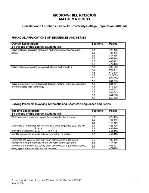
<strong>MCGRAW</strong>-<strong>HILL</strong> <strong>RYERSON</strong><br />
<strong>MATHEMATICS</strong> <strong>11</strong><br />
Correlation to Functions, Grade <strong>11</strong>, University/College Preparation (MCF3M)<br />
FINANCIAL APPLICATIONS OF SEQUENCES AND SERIES<br />
Overall Expectations<br />
By the end of this course, students will:<br />
Solve problems involving arithmetic and geometric sequences and<br />
series<br />
Sections<br />
6.1<br />
6.2<br />
6.3<br />
6.4<br />
6.5<br />
6.6<br />
Solve problems involving compound interest and annuities 7.1<br />
7.2<br />
7.3<br />
7.4<br />
7.5<br />
7.6<br />
Solve problems involving financial decision making, using spreadsheets<br />
or other appropriate technology<br />
7.2<br />
7.4<br />
7.5<br />
7.6<br />
7.7<br />
7.8<br />
Pages<br />
428-435<br />
436-446<br />
447-456<br />
457-464<br />
465-471<br />
472-478<br />
498-500<br />
501-5<strong>11</strong><br />
512-515<br />
516-525<br />
526-533<br />
534-543<br />
501-5<strong>11</strong><br />
516-525<br />
526-533<br />
534-543<br />
544-558<br />
559-570<br />
Solving Problems Involving Arithmetic and Geometric Sequences and Series<br />
Specific Expectations<br />
Sections Pages<br />
By the end of this course, students will:<br />
Write terms of a sequence, given the formula for the nth term 6.1<br />
6.2<br />
6.3<br />
428-435<br />
436-446<br />
447-456<br />
Determine a formula for the nth term of a given sequence (e.g., the nth 6.1<br />
6.2<br />
428-435<br />
436-446<br />
term of the sequence , , , . . . is )<br />
6.3<br />
447-456<br />
Identify sequences as arithmetic or geometric, or neither 6.3 447-456<br />
Determine the value of any term in an arithmetic or a geometric<br />
sequence, using the formula for the nth term of the sequence<br />
Determine the sum of the terms of an arithmetic or a geometric series,<br />
using appropriate formulas and techniques.<br />
6.2<br />
6.3<br />
6.5<br />
6.6<br />
436-446<br />
447-456<br />
465-471<br />
472-478<br />
Prepared by McGraw-Hill Ryerson, 300 Water St., Whitby, ON L1N 9B6<br />
May <strong>11</strong>, 2001<br />
1
Solving Problems Involving Compound Interest and Annuities<br />
Specific Expectations<br />
By the end of this course, students will:<br />
Derive the formulas for compound interest and present value, the<br />
amount of an ordinary annuity, and the present value of an ordinary<br />
annuity, using the formulas for the nth term of a geometric sequence<br />
and the sum of the first n terms of a geometric series<br />
Sections<br />
7.2<br />
7.3<br />
7.4<br />
7.5<br />
7.6<br />
Solve problems involving compound interest and present value 7.2<br />
7.3<br />
7.4<br />
Solve problems involving the amount and the present value of an<br />
ordinary annuity<br />
Demonstrate an understanding of the relationships between simple<br />
interest, arithmetic sequences, and linear growth<br />
Demonstrate an understanding of the relationships between compound<br />
interest, geometric sequences, and exponential growth<br />
7.5<br />
7.6<br />
7.1<br />
7.3<br />
7.2<br />
7.3<br />
Pages<br />
501-5<strong>11</strong><br />
512-515<br />
516-525<br />
526-533<br />
534-543<br />
501-5<strong>11</strong><br />
512-515<br />
516-525<br />
526-533<br />
534-543<br />
498-500<br />
512-515<br />
501-5<strong>11</strong><br />
512-515<br />
Solving Problems Involving Financial Decision Making<br />
Specific Expectations<br />
By the end of this course, students will:<br />
Analyse the effects of changing the conditions in long-term savings<br />
plans (e.g., altering the frequency of deposits, the amount of deposit,<br />
the interest rate, the compounding period, or a combination of these)<br />
(Sample problem: Compare the results of making an annual deposit of<br />
$1000 to an RRSP, beginning at age 20, with the results of making an<br />
annual deposit of $3000, beginning at age 50)<br />
Describe the manner in which interest is calculated on a mortgage (i.e.,<br />
compounded semi-annually but calculated monthly) and compare this<br />
with the method of interest compounded monthly and calculated<br />
monthly<br />
Generate amortization tables for mortgages, using spreadsheets or<br />
other appropriate software<br />
Analyse the effects of changing the conditions of a mortgage (e.g., the<br />
effect on the length of time needed to pay off the mortgage of changing<br />
the payment frequency or the interest rate)<br />
communicate the solutions to problems and the findings of<br />
investigations with clarity and justification<br />
Sections<br />
7.2<br />
7.4<br />
7.5<br />
7.6<br />
7.7<br />
7.8<br />
7.7<br />
7.8<br />
7.7<br />
7.8<br />
7.1<br />
7.2<br />
7.3<br />
7.4<br />
7.5<br />
7.6<br />
7.7<br />
7.8<br />
Pages<br />
501-5<strong>11</strong><br />
516-525<br />
526-533<br />
534-543<br />
544-558<br />
559-570<br />
544-558<br />
559-570<br />
544-558<br />
559-570<br />
498-500<br />
501-5<strong>11</strong><br />
512-515<br />
516-525<br />
526-533<br />
534-543<br />
544-558<br />
559-570<br />
Prepared by McGraw-Hill Ryerson, 300 Water St., Whitby, ON L1N 9B6<br />
May <strong>11</strong>, 2001<br />
2
TRIGONOMETRIC FUNCTIONS<br />
Overall Expectations<br />
By the end of this course, students will:<br />
Solve problems involving the sine law and the cosine law in oblique<br />
triangles<br />
Demonstrate an understanding of the meaning and application of radian<br />
measure<br />
Determine, through investigation, the relationships between the graphs<br />
and the equations of sinusoidal functions<br />
Solve problems involving models of sinusoidal functions drawn from a<br />
variety of applications<br />
Sections<br />
4.1<br />
4.2<br />
4.3<br />
4.4<br />
5.1<br />
5.2<br />
5.5<br />
5.6<br />
5.7<br />
5.8<br />
5.4<br />
5.5<br />
5.6<br />
5.3<br />
5.5<br />
5.6<br />
Pages<br />
266-275<br />
276-282<br />
283-295<br />
300-3<strong>11</strong><br />
328-340<br />
341-350<br />
367-377<br />
378-391<br />
393-401<br />
402-410<br />
363-366<br />
367-377<br />
378-391<br />
355-362<br />
367-377<br />
378-391<br />
Solving Problems Involving the Sine Law and the Cosine Law in Oblique Triangles<br />
Specific Expectations<br />
By the end of this course, students will:<br />
Determine the sine, cosine, and tangent of angles greater than 90°,<br />
using a suitable technique (e.g., related angles, the unit circle), and<br />
determine two angles that correspond to a given single trigonometric<br />
function value)<br />
Solve problems in two dimensions and three dimensions involving right<br />
triangles and oblique triangles, using the primary trigonometric ratios,<br />
the cosine law, and the sine law (including the ambiguous case)<br />
Sections<br />
4.2<br />
4.4<br />
5.2<br />
4.1<br />
4.3<br />
4.4<br />
Pages<br />
276-282<br />
300-3<strong>11</strong><br />
341-350<br />
266-275<br />
283-295<br />
300-3<strong>11</strong><br />
Understanding the Meaning and Application of Radian Measure<br />
Specific Expectations<br />
Sections Pages<br />
By the end of this course, students will:<br />
Define the term radian measure 5.1 328-340<br />
Describe the relationship between radian measure and degree measure 5.1 328-340<br />
Represent, in applications, radian measure in exact form as an<br />
5.1 328-340<br />
expression involving (e.g., , 2 ) and in approximate form as a real<br />
number (e.g., 1.05)<br />
Determine the exact values of the sine, cosine, and tangent of the<br />
special angles 0, , , , and their multiples less than or equal to 2<br />
Prove simple identities, using the Pythagorean identity,<br />
sin 2 x + cos 2 x = 1, and the quotient relation,<br />
5.2 341-350<br />
5.7 393-401<br />
Solve linear and quadratic trigonometric equations<br />
(e.g., 6 cos 2 x – sin x – 4 = 0) on the interval 0 x 2<br />
Demonstrate facility in the use of radian measure in solving equations<br />
and in graphing<br />
5.8 402-410<br />
5.5<br />
5.6<br />
5.8<br />
367-377<br />
378-391<br />
402-410<br />
Prepared by McGraw-Hill Ryerson, 300 Water St., Whitby, ON L1N 9B6<br />
May <strong>11</strong>, 2001<br />
3
Investigating the Relationships Between the Graphs and the Equations of Sinusoidal Functions<br />
Specific Expectations<br />
By the end of this course, students will:<br />
Sketch the graphs of y = sin x and y = cos x, and describe their periodic<br />
properties<br />
Determine, through investigation, using graphing calculators or<br />
graphing software, the effect of simple transformations (e.g.,<br />
translations, reflections, stretches) on the graphs and equations of y =<br />
sin x and y = cos x<br />
Determine the amplitude, period, phase shift, domain, and range of<br />
sinusoidal functions whose equations are given in the form y = a sin(kx<br />
+ d) + c or y = a cos(kx + d) + c<br />
Sketch the graphs of simple sinusoidal functions [e.g., y = a sin x, y =<br />
cos kx, y = sin(x + d), y = a cos kx + c]<br />
Write the equation of a sinusoidal function, given its graph and given its<br />
properties<br />
Sketch the graph of y = tan x; identify the period, domain, and range of<br />
the function; and explain the occurrence of asymptotes<br />
Sections<br />
Pages<br />
5.4 363-366<br />
5.5<br />
5.6<br />
367-377<br />
378-391<br />
5.6 378-391<br />
5.4<br />
5.5<br />
5.6<br />
5.5<br />
5.6<br />
363-366<br />
367-377<br />
378-391<br />
367-377<br />
378-391<br />
5.4 363-366<br />
Solving Problems Involving Models of Sinusoidal Functions<br />
Specific Expectations<br />
By the end of this course, students will:<br />
Determine, through investigation, the periodic properties of various<br />
models (e.g., the table of values, the graph, the equation) of sinusoidal<br />
functions drawn from a variety of applications<br />
Explain the relationship between the properties of a sinusoidal function<br />
and the parameters of its equation, within the context of an application,<br />
and over a restricted domain<br />
Predict the effects on the mathematical model of an application<br />
involving sinusoidal functions when the conditions in the application are<br />
varied<br />
Pose and solve problems related to models of sinusoidal functions<br />
drawn from a variety of applications, and communicate the solutions<br />
with clarity and justification, using appropriate mathematical forms<br />
Sections<br />
5.3<br />
5.5<br />
5.6<br />
5.5<br />
5.6<br />
5.5<br />
5.6<br />
5.5<br />
5.6<br />
Pages<br />
355-362<br />
367-377<br />
378-391<br />
367-377<br />
378-391<br />
367-377<br />
378-391<br />
367-377<br />
378-391<br />
Prepared by McGraw-Hill Ryerson, 300 Water St., Whitby, ON L1N 9B6<br />
May <strong>11</strong>, 2001<br />
4
TOOLS FOR OPERATING AND COMMUNICATING WITH FUNCTIONS<br />
Overall Expectations<br />
By the end of this course, students will:<br />
Demonstrate facility in manipulating polynomials, rational expressions,<br />
and exponential expressions<br />
Demonstrate an understanding of inverses and transformations of<br />
functions and facility in the use of function notation<br />
Communicate mathematical reasoning with precision and clarity<br />
throughout the course<br />
Sections<br />
1.1<br />
1.2<br />
1.3<br />
1.4<br />
1.5<br />
1.6<br />
1.7<br />
1.8<br />
1.9<br />
2.1<br />
2.2<br />
2.3<br />
2.4<br />
2.5<br />
3.1<br />
3.2<br />
3.3<br />
3.4<br />
3.5<br />
3.6<br />
3.7<br />
throughout<br />
book<br />
Pages<br />
4-10<br />
<strong>11</strong>-18<br />
19-26<br />
28-34<br />
35-43<br />
44-52<br />
53-61<br />
62-69<br />
72-81<br />
100-109<br />
<strong>11</strong>0-<strong>11</strong>9<br />
120-133<br />
135-142<br />
144-152<br />
170-181<br />
182-183<br />
184-193<br />
194-207<br />
208-220<br />
221-232<br />
233-243<br />
throughout<br />
book<br />
Manipulating Polynomials, Rational Expressions, and Exponential Expressions<br />
Specific Expectations<br />
Sections Pages<br />
By the end of this course, students will:<br />
Solve first-degree inequalities and represent the solutions on number 1.9 72-81<br />
lines<br />
Add, subtract, and multiply polynomials 1.4 28-34<br />
Determine the maximum or minimum value of a quadratic function<br />
whose equation is given in the form y = ax 2 + bx + c, using the algebraic<br />
method of completing the square<br />
Identify the structure of the complex number system and express<br />
complex numbers in the form a + bi, where i 2 = –1 (e.g., 4i, 3 – 2i)<br />
Determine the real or complex roots of quadratic equations, using an<br />
appropriate method (e.g., factoring, the quadratic formula, completing<br />
the square), and relate the roots to the x-intercepts of the graph of the<br />
corresponding function<br />
Add, subtract, multiply, and divide rational expressions, and state the<br />
restrictions on the variable values<br />
2.2 <strong>11</strong>0-<strong>11</strong>9<br />
2.1 100-109<br />
2.3 120-133<br />
1.5<br />
1.6<br />
1.7<br />
1.8<br />
1.1<br />
Simplify and evaluate expressions containing integer and rational<br />
exponents, using the laws of exponents<br />
1.2<br />
Solve exponential equations (e.g., 4 x = 8 x + 3 , 2 2x – 2 x = 12). 1.1<br />
1.2<br />
35-43<br />
44-52<br />
53-61<br />
62-71<br />
4-10<br />
<strong>11</strong>-18<br />
4-10<br />
<strong>11</strong>-18<br />
Prepared by McGraw-Hill Ryerson, 300 Water St., Whitby, ON L1N 9B6<br />
May <strong>11</strong>, 2001<br />
5
Understanding Inverses and Transformations and Using Function Notation<br />
Specific Expectations<br />
Sections Pages<br />
By the end of this course, students will:<br />
Define the term function 3.1 170-181<br />
Demonstrate facility in the use of function notation for substituting into<br />
and evaluating functions<br />
Determine, through investigation, the properties of the functions defined<br />
by ƒ(x) = [e.g., domain, range, relationship to ƒ(x) = x 2 ] and ƒ(x) =<br />
[e.g., domain, range, relationship to ƒ(x) = x.]<br />
Explain the relationship between a function and its inverse (i.e.,<br />
symmetry of their graphs in the line y = x; the interchange of x and y in<br />
the equation of the function; the interchanges of the domain and range),<br />
using examples drawn from linear and quadratic functions, and from the<br />
throughout<br />
Ch. 3<br />
throughout<br />
Ch. 3<br />
3.2 182-183<br />
3.5 208-220<br />
functions ƒ(x) = and ƒ(x) =<br />
Represent inverse functions, using function notation, where appropriate 3.5 208-220<br />
Represent transformations (e.g., translations, reflections, stretches) of<br />
the functions defined by ƒ(x) = x, ƒ(x) = x 2 , ƒ(x) = , ƒ(x) = sin x, and<br />
ƒ(x) = cos x, using function notation<br />
Describe, by interpreting function notation, the relationship between the<br />
graph of a function and its image under one or more transformations<br />
State the domain and range of transformations of the functions defined<br />
by ƒ(x) = x, ƒ(x) = x 2 , ƒ(x) = , ƒ(x) = sin x, and ƒ(x) = cos x<br />
Communicating Mathematical Reasoning<br />
Specific Expectations<br />
By the end of this course, students will:<br />
Explain mathematical processes, methods of solution, and concepts<br />
clearly to others<br />
Present problems and their solutions to a group, and answer questions<br />
about the problems and the solutions<br />
Communicate solutions to problems and to findings of investigations<br />
clearly and concisely, orally and in writing, using an effective integration<br />
of essay and mathematical forms<br />
Demonstrate the correct use of mathematical language, symbols,<br />
visuals (e.g., diagrams, graphs), and conventions<br />
Use graphing technology effectively (e.g., use appropriate menus and<br />
algorithms; set the graph window to display the appropriate section of a<br />
curve)<br />
3.3<br />
3.4<br />
3.5<br />
3.6<br />
3.7<br />
3.3<br />
3.4<br />
3.5<br />
3.6<br />
3.7<br />
3.3<br />
3.4<br />
3.5<br />
3.6<br />
3.7<br />
Sections<br />
throughout<br />
book<br />
throughout<br />
book<br />
throughout<br />
book<br />
throughout<br />
book<br />
throughout<br />
book<br />
184-193<br />
194-207<br />
208-220<br />
221-232<br />
233-243<br />
184-193<br />
194-207<br />
208-220<br />
221-232<br />
233-243<br />
184-193<br />
194-207<br />
208-220<br />
221-232<br />
233-243<br />
Pages<br />
throughout<br />
book<br />
throughout<br />
book<br />
throughout<br />
book<br />
throughout<br />
book<br />
throughout<br />
book<br />
Prepared by McGraw-Hill Ryerson, 300 Water St., Whitby, ON L1N 9B6<br />
May <strong>11</strong>, 2001<br />
6