ABOUT THE ANOVA TEST

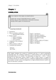
Chapter 6: Analysis of Variance 

1 

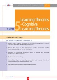
Chaptter 6:: 

ANALSYIIS OF VARIIANCE 

Upon completion of this chapter, you should be able to: 

 

 

 

 

 

 

define the OneWay ANOVA 

explain the logic of OneWay ANOVA 

compute Oneway ANOVA using a formula 

identify the assumptions for using the OneWay ANOVA 

compute Oneway ANOVA using SPSS 

interpret the OneWay ANOVA output using an online calculator 

 

 

 

 

 

CHAPTER OVERVIEW 

About the Oneway Anova test 

The logic of the Oneway Anova 

Computing the F-test 

Assumptions for using the Oneway 

Anova 

Example: Using the SPSS to 

compute the Oneway ANOVA 

Chapter 1: Introduction 

Chapter 2: Descriptive Statistics 

Chapter 3: The Normal Distribution 

Chapter 4: Hypothesis Testing 

Chapter 5: T-test 

Chapter 6: Oneway Analysis of Variance 

Chapter 7: Correlation 

Chapter 8: Chi-Square 

This chapter introduces you to the Oneway Anova beginning with its logic and the 

formula that explains the statistical tool. You do not need to remember the formula but 

rather the meaning of the formula. The tool is often used to test the differences between 

two or more means. You should give due consideration to the assumptions underlying the 

use of the statistical tool. SPSS provides a convenient and quick way to compute the F- 

statistic which will tell you whether the differences between means is significant.


2 

About the ANOVA Test 

In educational research, we often are involved in finding out whether there are 

differences between groups. For example, is there a difference between males and 

female, between rural and urban students and so forth. As we discussed in Chapter 5, 

the t-test was used to compare differences of means between two groups, such as 

comparing outcomes between a control and treatment group in an experimental 

study. Suppose you are interested in comparing the means of three groups (i.e k = 3) 

rather than two. 

You might be tempted to use multiple t-test and compare the means 

separately; i.e. you compare the means of Group 1 and 2 followed by Group 1 and 3 

and so forth. What is the danger of doing this? Multiple t-tests enhances the likelihood 

of committing Type 1 error (i.e. Claiming that two means are not equal when in fact 

they are equal). In other words, you reject a null hypothesis when it is TRUE. On a 

practical level, using the t-test to compare many means is a cumbersome process in 

terms of the calculations involved. 

EXAMPLE: 

Let us look at this example which shows the results of a study on Attitude Towards 

Homework among students of varying ability levels. Subjects were divided into three 

groups: High Ability, Average Ability and Low Ability. The total sample size is 505 

students. You need a special class of statistical techniques called the OneWay 

Analysis of Variance or OneWay ANOVA which we will discuss here. 

ATTITUDES TOWARDS HOMEWORK AMONG 14 YEAR OLD STUDENTS 

Group N Mean Std. Dev. Std. Error 95 Pct Conf. Int for Mean 

High ability 220 13.03 3.17 0.12 12.79 TO 13.27 

Average ability 212 11.99 2.93 0.11 11.77 TO 12.21 

Low ability 73 9.54 3.50 0.40 8.73 TO 10.36 

Interpretation of the Table Above 

 

What do the three Means tell you? High ability students have the highest 

mean (13.03), while low ability students have the lowest mean (9.54). Average 

ability students fall in the middle, with a mean of 11.99. 

 

What do the three Standard Deviations tell you? Note that the standard 

deviation for high ability (3.17) and average ability (2.93) students is fairly


3 

close while low ability students have a somewhat bigger standard deviation of 

3.50. 

 

 

 

What do the three Standard Errors tell you? Refer to the table, and you 

will notice that that there is a column called 'standard error'. What is the 

standard error? The standard error is a measure of how much the sample 

means vary if you were to take repeated samples from the same population. 

The first two groups contain > 200 students each, the standard error of the 

mean for each of these groups is fairly small. It is 0.12 for high ability students 

and 0.11 for average ability students. However, the standard error for the low 

ability group is comparatively high = 0.40. Why? The smaller number of low 

ability students (n=73) and the larger standard deviation explains why the 

standard error is larger. 

What does 95 Pct Conf. Int for Mean? The last column displays the 

'confidence interval'. What is the confidence interval? It is the range which is 

likely to contain the true population value or mean. If you take repeated 

samples of 14 year students from the same population of 14 year old students 

in the country and calculate their mean, there is a probability that 95% of them 

should include the unknown population value or mean. For example, you can 

be 95% confident that, in the population, the mean of high ability students is 

somewhere between 12.79 and 13.27. Similarly, you can be 95% confident 

that, in the population, the mean of low ability students is somewhere between 

8.73 and 10.36. 

You will notice that the confidence interval is wider for low ability students 

(i.e. 1.63) compared to confidence interval for high ability students (i.e. 0.48). 

Why? This is due to the larger standard error (0.40) obtained by low ability 

students. Since, the confidence interval depends on the standard error of the 

mean, the confidence interval for low ability students is wider than for high 

ability students. So, the larger the standard error, the wider will be the 

confidence interval. Makes sense doesn't it! 

At the heart of ANOVA is the concept of VARIANCE. What is variance? Most of 

you would say, it the standard deviation squared!. Yes, that is correct. Focus is on two 

types of variance: 

 

 

Between-Group Variance, i.e. If there are THREE groups, it is the variance 

between the three groups. 

Within-Group Variance, i.e. If in each group there are 30 subjects, it is the 

variance of scores within subjects in that group. 

The F-value is a ratio of the Between-Group 

Variance and Within-Group Variance


4 

If the F-value is significant, it tells us that the population means are probably NOT 

ALL EQUAL and you reject the null hypothesis. Next, you have to locate where the 

significant lies or which of the means are significantly different. You have to use poshoc 

analysis to determine this. 

LEARNING ACTIVITY 

a) When would you use Oneway ANOVA and not the t-test 

to compare means? 

b) What is the standard error? Why does the standard error 

vary? 

c) Explain "95 Pct Conf. Int for Mean". 

The Logic of the ONEWAY ANOVA 

A researcher was interested in finding out whether there are differences in 

creative thinking among 12 year students from different socio-economic backgrounds. 

Creative thinking was measured using The Torrance Test of Creative Thinking 

consisting of 5 items while socio-economic status (SES) was measured using 

household income. Socio-economic status or SES was divided into 3 Groups (High, 

Middle and Low). The null hypothesis generated is that all three groups will have the 

same mean score on the creative test. In formula terms, if we use the symbol μ 

[pronounced as ‘mew’] to represent the average score, the null hypothesis is 

expressed through the following notation: 

The NULL HYPOTHESIS is represented as follows: 

Ho : μ1 = μ2 = μ3 

Mean 

4.00 

High SES Middle SES Low SES


5 

The null hypothesis states that the mean of high ability, average ability and low ability 

students is the same; i.e. is equal to 4.00 

To test the null hypothesis, the Oneway Analysis of Variance is used. The Oneway 

ANOVA is a statistical technique used to test the null hypothesis that several 

populations means are equal. The word 'variance' is used because it examines the 

variability in the sample. In other words, how much do the scores of individual 

students vary from the mean. Based on the variability or variance, it determines 

whether there is reason to believe that the population means are not equal. In our 

example, does creativity vary between the three groups of 12 year old students. 

The ALTERNATIVE HYPOTHESIS is represented as follows: 

Ha: µ1 ≠ µ2 ≠ µ2 

Mean 

4.12 4.37 

4.00 

3.85 

‘ 

High SES Middle SES Low SES 

The alternative hypothesis states that there is a difference between the three 

groups of students (see Figure above). However, the alternative hypothesis does not 

state which groups differ from one another. It just says that the means of each group 

are not all the same; or at least one of the groups differs from the others. 

Are the means really different? We need to figure out whether the observed 

differences in the sample means are attributed to just the natural variability among 

sample means or whether there is reason to believe that the three groups of students 

have different means in the population. In other words, are the differences due to 

chance or there is a 'real' difference.


6 


a) What does the word 'variance' mean in the Oneway 

Analysis of Variance? 

b) Why would you use the Oneway ANOVA rather than 

the t-test? 

BETWEEN GROUP AND WITHIN GROUP VARIANCE 

As mentioned earlier, the researcher was interested in determining whether 

there were differences in creativity between students from different socio-economic 

backgrounds; i.e. High SES, Middle SES and Low SES. To determine if there are 

significant differences between the three means, you have to compute the F-ratio or F- 

test. To compute the F-ratio you have to use two types of variances: 

 

 

Between Group Variance or the variability between group means. 

Within Group Variance or the variability of the observations (or scores) within 

a group (around a particular group's mean) 

a) Between Group Variance 

The diagram above presents the results of the study. Let us look more closely at the 

two types of variability or variance. Note that each of the three groups has a mean 

which is also known as the sample mean. 

 

 

 

The high SES group has a mean of 4.12 for the creativity test 

The middle SES group has a mean of 4.37 for the creativity test 

The low SES had a mean of 3.85 for the creativity test. 

b) Within Group Variance 

Within group variance or variability is a measure of how much the 

observations or scores within a group vary. It is simply the variance of the 

observations or scores within a group or sample, and it is used to estimate the variance 

within a group in the population. Remember, ANOVA requires the assumption that all 

of the groups have the same variance in the population. Since you do not know if all 

of the groups have the same mean, you cannot just calculate the variance for all of the 

cases together. You must calculate the variance for each of the groups individually 

and then combine these into an "average" variance. 

Within group variance for the example shows that the 313 students within the 

high SES group have different scores, the 297 students within the middle SES group 

have different scores and the 340 students within the low SES also have different


7 

scores. Among the three groups, there is slightly greater variability or variance among 

Low SES subjects (SD = 1.31) compared to High SES subjects with a SD of 1.28. 


a) What do you mean by "between group variance"? 

b) What do you mean by "within group variance"? 

Computing the F-Test 

The F-test or the F-ratio is a measure of how different the means are relative to 

the variability or variance within each sample. The larger the F value, the greater the 

likelihood that the differences between means are due to something other than chance 

alone; i.e. real effects or the means are significantly different from one another. 

Below is the summarised formula for computing the F statistic or F-ratio: 

F = 

Between Mean Square 

Within Mean Squares 

Based on the study (see the Table for results) about the relationship between 

creativity and socio-economic status of subject, computation of the F-statistics is as 

follows: 

High SES Middle SES Low SES 

Mean = 4.12 4.37 3.85 

SD = 1.28 1.30 1.31 

n = 313 297 340


8 

STEPS FOR COMPUTING THE F STATISTICS OR F-RATIO: 

Step 1: 

Computation of the Between Sum of Squares (BSS) 

The first step is to calculate the variation between groups by comparing the 

mean of each SES group with the Mean of the Overall Sample (the mean score on the 

test for all students in this sample is 4.00). 

BSS = n1 ( x1 – x)² + n2 (x2 – x)² + n3 (x2 – x)² 

This measure of between-group variance is referred to as "Between Sum of 

Squares" (or BSS). This is calculated by adding up (for all the 3 groups), the 

difference between the group's mean and the overall population mean (4.00), 

multiplied by the number of cases (i.e. n) in each group. 

Between Sum of Squares (BSS) 

= No. of students x (Mean of Group 1 – Overall Mean)² + No. 

of students x (Mean of Group 2 – Overall Mean) ² + No. of 

students x (Mean of Group 3 – Overall Mean) ² 

= 313 (4.12 – 4.00)² + 297 (4.37 – 4.00)² + 340 (3.99 – 

4.00)² 

= 4.51 + 40.66 + 0.034 = 45.21 

Degrees of freedom: 

This sum of squares has a number of degrees of freedom equal to the number of 

groups minus 1. In this case, dfB = (3-1) = 2 

Step 2: 

Computation of the Between Mean Squares (BMS) 

BSS 45.21 

Between Mean Squares = = = 22.61 

df 2 

Divide the BSS figure (45.21) by the number of degrees of freedom (2) to get our 

estimate of the variation between groups, referred to as "Between Mean Squares".


9 

Step 3: 

Computation of the Within Sum of Squares (WSS) 

To measure the variation within groups, we find the sum of the squared deviation 

between scores on the Torrance Creative Test and the group average, calculating 

separate measures for each group, then summing the group values. This is a sum 

referred to as the "Within Sum of Squares" (or WSS). 

WSS = ( n 1 – 1) SD1² + ( n 2 – 1) SD2² + ( n 3 – 1 ) SD3² 

Within Sum of Squares (WSS) 

= (Degrees of Freedom of Group 1 minus 1) x SD² + (Degrees 

of Freedom of Group 2 minus 1) x SD² + (Degrees of Freedom 

of Group 3 minus 1) x SD² 

= (313 – 1) 1.28² + (297 – 1) 1.30² + (340 – 1) 1.31² 

= 511.18 + 500.24 + 581.76 

= 1070.18 

Degrees of freedom: 

As in Step 1, we need to adjust the WSS to transform it into an estimate of population 

variance, an adjustment that involves a value for the number of degrees of freedom 

within. To calculate this, we take a value equal to the number of cases in the total 

sample (N = 950), minus the number of groups (k = 3), i.e. 950 - 3 = 947 

Step 4: 

Computation of the Within Mean Squares (WMS) 

Divide the WSS figure (1071.18) by the degrees of freedom (N - k = 947) to get an 

estimate of the variation within groups referred to as "Within Mean Squares" 

WSS 1071.18 

Within Mean Squares = = = 1.13 

(WMS) df 947


10 

Step 5: 

Computation of the F test statistic 

This calculation is relatively straightforward. Simply divide the Between Mean 

Squares (BMS), the value obtained in step 1, by the Within Mean Squares (WMS), 

the value calculated in step 2. 

Between Mean Square 22.61 

F = = = 20.0 

Wtihin Mean Squares 1.13 

Step 6: 

To Reject or Not Reject the Hypothesis 

To determine if the F statistics is sufficiently large to Reject the null hypothesis, you 

have to determine the critical value for the F statistics by referring to the F 

distribution. There are two degrees of freedom: 

k -1 which is numerator [i.e. 3 group minus 1 = 3- 1 = 2] 

N -k which is the denominator [i.e. no. of subjects minus number of groups = 

950 - 3 = 947 

The critical value is 3.070 which is 2 df by 120 df (the distribution provided 

in most textbooks has a maximum of 120 df. You use it for any denominator 

exceeding 120 df). 

Extract from Table of Critical Values for the F Distribution 

df2 

df1 1 2 3 4 

96 3.940 3.091 2.699 2.466 

97 3.939 3.090 2.698 2.465 

98 3.938 3.089 2.697 2.465 

99 3.937 3.088 2.696 2.464 

100 3.936 3.087 2.696 2.463 

120 3.920 3.070 2.680 2.450


11 

Finally, compare the F-statistics (20.0) with the critical value 3.07. At at p = 0.05. the 

F-statistics is larger (>) than the critical value and hence there is strong evidence to 

Reject the null hypothesis, indicating that there is a significant difference in creativity 

among the three groups of students. While the F-statistic assesses the null hypothesis 

of equal means, it does not address the question of which means are different. For 

example, all three groups may be different significantly, or two may be equal but 

differ from the third. To establish which of the 3 Groups are different, you have to 

follow up with post hoc comparison or tests. 

Step 7: 

Post Hoc Comparisons or Tests 

There are many techniques available for post hoc comparisons and they are as 

follows: 

Least square difference (LSD) 

Duncan 

Dunnett 

Tukey's honest square difference (HSD) 

Scheffe 

Tukey's HSD 

Mean1 Mean2 

Mean1 

Mean2 

Mean3 * 

Mean3 

Tukey HSD 

The Tukey's HSD runs a series of Tukey's post hoc tests, which are like a series of t- 

tests. However, the post-hoc tests are more stringent than the regular t-tests. It 

indicates how large an observed difference must be for the multiple comparison 

procedure to call it significant. Any absolute difference between means has to exceed 

the value of HSD to be statistically significant. 

Most statistical programmes will give you an output in the form of a table as 

shown on the right. Group means listed as a matrix. An asterik (*) indicates which 

pairs of means are significantly different. 

Note that the only the mean of Group 3 is significantly different from Group 1. 

In other words, High SES (M = 4.12) subject scored significantly higher on creativity 

than Low SES (M = 3.85) subjects. There was no significant difference between High 

SES and Middle SES subjects nor was there a significant difference between Middle 

SES and Low SES subjects.


12 

Assumptions for Using the ONEWAY ANOVA 

Just like all statistical tools, there are certain assumptions that have to be met 

for their usage. The following are several assumptions for using the One-Way 

ANOVA: 

A) Independent Observations or Subject: 

Are the observations in each of the groups independent ? This means that the 

data must be independent. On other words, a particular subject should belong to only 

group. If there are three groups, they should be made up of separate individuals so 

that the data are truly independent. 

If the same subject belongs to the same group and tested twice such as in the 

case of a pretest and posttest design, you should instead use the Repeated Measure 

One-Way ANOVA [Not discussed in this course]. 

B) Simple Random Samples: 

The samples taken from the population under consideration are randomly selected 

(Refer to Chapter 1 for random selection techniques). 

C) Normal Populations: 

For each population, the variable under consideration is normally distributed [Refer to 

Chapter 2 for techniques to determine normality of distribution). In other words, to 

use the OneWay ANOVA you have to ensure that that the distributions for each of the 

groups are normal. The analysis of variance is robust if each of the distributions are 

symmetric or if all the distributions are skewed in the same direction. This assumption 

can be tested by running several normality tests. 

1. Normality Tests Using Skewness 

Independent variable group Statistic Std. Error 

Mean 43.82 2.20 

Group 1 Skewness .973 .491 

Kurtosis .341 .953 

Mean 60.14 2.71 

Group 2 Skewness -.235 .597 

Kurtosis -1.066 1.154 

Mean 64.75 3.61 

Group 3 Skewness -.407 .564 

Kurtosis -1.289 1.091


13 

Refer to the Table above which show the means, skewness and kurtosis for three 

groups. The skewness and kurtosis scores indicate that the scores in Group 1 and 

Group 2 are normally distributed. There is some positive skewness in Group 1 

2) Normality Tests Using Kolmogorov-Smirnov Statistic 

Tests of Normality 

Kolmogorov-Smirnov (a) 

Shapiro-Wilks 

Independent variable Statistic df Sig. Statistic df Sig. 

group 

Group 1 .206 22 .016 .912 22 .055 

Group 2 .166 14 .200(*) .940 14 .442 

Group 3 .151 16 .200(*) .900 16 .084 

(*) This is a lower bound of the true significance. 

a. Lilliefors Significance Correction 

The Shapiro-Wilks normality tests indicate that the scores are normally distributed in 

each of the three conditions. The Kolmogorov-Statistic is significant, but that statistic 

is more appropriate for larger sample sizes. 

D) Homogeneity of Variance: 

Test of Homogeneity of Variances 

Dependent variable 

Levene df1 df2 Sig. 

Statistics 

2.284 2 49 113 

Just like you did with the t-test, the Levene's test of homogeneity of variance is used 

for the OneWay ANOVA and is show in the Table below. The p-value which is 0.113 

is greater than the alpha of 0.05. Hence, it can be concluded that the variances are 

homogeneous which is reported as Levene (2, 49) = 2.28, p = .113.


14 


a) When would you use Oneway ANOVA and not the t-test 

to compare means? 

b) What are the assumptions that must be met when using 

ANOVA? 

EXAMPLE: Using SPSS to Compute Oneway ANOVA 

In the COPs study in 2006, a team of researchers administered an Inductive 

Reasoning Test to a sample of 946 eighteen year old Malaysians. One of the 

independent variables examined was socio-economics status (SES). There were 

FOUR SES groups: very high SES, high SES, middle SES and low SES. Researchers 

were interested in answering this research question: 

Research Question: 

Is there a significant difference in inductive reasoning ability between adolescents of 

different socio-economic status? 

Null Hypothesis: Ho: μ1 = μ2 = μ3 = μ4 

Alternative Hypothesis: Ho: µ1 ≠ µ2 ≠ µ3 ≠ µ4


15 

Procedure for the Oneway ANOVA with post-hoc anaylsis Using SPSS 

1. Select the Analyze menu. 

2. Click on Compare Means and One-Way ANOVA ..... to open the One- 

Way NOVA dialogue box. 

3. Select the Dependent variable (i.e. inductive reasoning) and click on the 

button to move the variable into the Dependent List: box. 

4. Select the Independent variable (i.e. SES) and click on the button to 

move the variable into the Factor: box. 

5. Click on the Options .....command pushbutton to open the One-Way 

ANOVA: Options sub-dialogue box. 

6. Click on the check boxes for Descriptive and Homogeneity-of-variance. 

7. Click on Continue. 

8. Click on the Post Hoc .... command pushbutton to open the One-Way 

ANOVA: Post Hoc Multiple Comparisons sub-dialogue box. You will 

notice that a number of multiple comparison options are available. In this 

example you will use the Tukey's HSD multiple comparison test. 

9. Click on the check box for Tukey. 

10. Click on Continue and then OK. 

#1. Testing for Homogeneity of Variance 

Before you conduct the Oneway ANOVA, you have to make sure that your data meet 

the relevant assumptions of using Oneway ANOVA. Let’s first look at the test of 

homogeneity of variances, since satisfying this assumption is necessary for 

interpreting ANOVA results. 

Levene’s test for homogeneity of variances assesses whether the population variances 

for the groups are significantly different from each other. The null hypothesis states 

that the population variances are equal: 

Ho: μ1 = μ2 = μ3 = μ4 

Levene's Test for Homogeneity of Variance 

F df1 df2 Sign 

.383 3 942 .765 

The table above is the SPSS output for the Levene's test. Note that the Levene F 

statistic has a value of 0.383 and a p-value of 0.756. Since p is greater than α = 0.05


16 

(i.e. 0.756 > 0.05); we Do Not Reject the null hypothesis. Hence, we can conclude 

that the data does not violate the homogeneity-of-variance assumption. 

#2. Means and Standard Deviations 

Another SPSS output is the "Descriptives" table which presents the means and 

standard deviations of each group (see table). You will notice that the means are not 

all the same. This relatively simple conclusion, however, actually raises more 

questions. See if you can answer these questions: 

INDUCTIVE 

DESCRIPTIVES 

N Mean Std. Deviation Std. Error 

Low SES 258 8.0194 3.4228 .2131 

Middle SES 304 8.4967 3.2680 .1874 

High SES 214 8.7850 3.3735 .2306 

Very High SES 170 8.4989 3.3382 .1085 

Is „middle SES‟ (M = 8.49) different from „low SES‟ (M = 8.01)? 

Is “high SES” (M = 8.78) different from “middle SES” (M = 8.49)? 

Is “very high SES” (M = 8.87) different from “low SES” (M = 8.01)? 

As you may have realised, just by looking at the ‘Descriptives’ table, the group means 

cannot tell us decisively if significant differences exist. What is the next step? 

#3. Significant Differences 

Having concluded that the assumption of homogeneity of variance has been, the 

means and standard deviations of each of the four groups have been computed; the 

next step is to determine whether SES influences inductive reasoning. You are 

seeking to establish whether the four means are 'equal'.


17 

Sum of squares df Mean squares F Sig. 

Between groups 100.34 3 33.445 3.021 .029 

Within groups 10430.165 942 11.072 

Total 10530.499 945 

What does the table above indicate? 

 

 

 

 

The ‘Between groups’ row shows that the df is 3 (i.e. k - 1 = 4 – 1 = 3) and the 

mean square is 33.445. 

The ‘Within groups’ row shows that the df is 942 (N - k = 946 – 4 = 942) and 

the mean square is 11.072. 

If you divide 33.444 by 11.072 you will get the F value of 3.021 which is 

significant at 0.029. 

Since, 0.029 is < than α = 0.05, we can Reject the Null Hypothesis and accept 

the alternative hypothesis. You can conclude that there is a significant 

difference in inductive reasoning between the four SES groups. But which 

group? 

#4. Multiple Comparisons 

Having obtained a significant result, you can go further and determine using a posthoc 

test, where the signifiance lies. There are many different kinds of post-hoc tests, 

that examine which means are different from each other. One commonly used 

procedure is Tukey’s Honestly Significant Difference test (HSD). The Tukey test 

compares all pairs of group means and the results are shown in the ‘Multiple 

Comparisons’ table below.


18 

Dependent Variable: INDUCTIV 

Tukey HSD 

Mean 

Difference (I-J) Std. Error Sig. 

1.00 2.00 -.4773 .2817 .326 

3.00 -.7657 .3077 .062 

4.00 -.8512 .3287 .047 

2.00 1.00 -.4773 .2817 .326 

3.00 -.2883 .2969 .766 

4.00 -.3739 .3187 .644 

3.00 1.00 .7657 .3077 .062 

2.00 .2883 .2969 .766 

4.00 - 8.5542E-02 .3419 .995 

4.00 1.00 .8512 .3287 .047 

2.00 .3739 .3187 .644 

3.00 8.554E-02 .3419 .995 

1 = Low SES 

2 = Middle SES 

3 = High SES 

4 = Very High SES 

Note that each mean is compared to every other mean thrice so the results are 

essentially repeated in the table. Interpreting the table reveals that: 

There is a significant difference ONLY between ‘Low SES’ subjects (Mean = 8.01) 

and “Very High’ SES subjects (Mean = 8.87) at p = 0.047. i.e. Very High SES scored 

significantly higher than "Low SES" at p = 0.047. There are no significant differences 

between the other groups.


19 


A study was conducted to determine the effectiveness of 

the collaborative method in teaching primary school 

mathematics among pupils of varying ability levels. The 

performance of 18 pupils on a mathematics posttest is 

presented below: 

Low Ability Pupils Middle Ability Pupils High Ability Pupils 

45 55 59 

58 42 54 

61 41 62 

59 48 57 

49 36 48 

63 44 65 

Compute a OneWAY Anova and based on the output answer the 

following questions: 

a) Comment on the mean and standard deviation for the three 

groups. 

b) Is there a significant difference in mathematics performance 

between students of different ability levels? 

c) What is the p value? 

d) What is the F ratio or F value? 

e) Interpret the Tukey HSD


20 


A researcher conducted a study to assess the the level of 

knowledge possessed by university students regarding 

the rights and responsibilities as citizens. Students 

completed a standardised test. Major for students was 

also recorded. Data in terms of percent correct is 

recorded below for 32 students. Compute the OneWay 

Anova test for the data provided below. 

Education Management Social Science Computer Science 

62 7 42 80 

81 49 52 57 

75 63 31 87 

58 68 80 64 

67 39 22 28 

48 79 71 29 

26 40 68 62 

36 15 76 45 

Based on the output, answer the following questions: 

1. What is your computed answer? 

2. What would be the null hypothesis in this study? 

3. What would be the alternate hypothesis? 

4. What probability level did you choose and why? 

5. What were your degrees of freedom? 

6. Is there a significant difference between the four testing 

conditions? 

7. Interpret your answer. 

8. If you have made an error, would it be a Type I or a Type II error? 

Explain your answer. 

--------000----------

ABOUT THE ANOVA TEST

Create successful ePaper yourself

Delete template?

Save as template?