For t - ECE Users Pages - Georgia Institute of Technology
For t - ECE Users Pages - Georgia Institute of Technology
For t - ECE Users Pages - Georgia Institute of Technology

You also want an ePaper? Increase the reach of your titles
YUMPU automatically turns print PDFs into web optimized ePapers that Google loves.
<strong>ECE</strong> 4813<br />
Semiconductor Device and Material<br />
Characterization<br />
Dr. Alan Doolittle<br />
School <strong>of</strong> Electrical and Computer Engineering<br />
<strong>Georgia</strong> <strong>Institute</strong> <strong>of</strong> <strong>Technology</strong><br />
As with all <strong>of</strong> these lecture slides, I am indebted to Dr. Dieter Schroder from Arizona State<br />
University for his generous contributions and freely given resources. Most <strong>of</strong> (>80%) the<br />
figures/slides in this lecture came from Dieter. Some <strong>of</strong> these figures are copyrighted and can be<br />
found within the class text, Semiconductor Device and Materials Characterization. Every serious<br />
microelectronics student should have a copy <strong>of</strong> this book!<br />
<strong>ECE</strong> 4813 Dr. Alan Doolittle
Defects<br />
Types <strong>of</strong> Defects<br />
Defect Etching<br />
Generation – Recombination<br />
Capacitance Transients<br />
Deep Level Transient Spectroscopy<br />
<strong>ECE</strong> 4813 Dr. Alan Doolittle
Metal<br />
Impurities<br />
Recombination<br />
Centers<br />
DRAM Refresh<br />
Failures<br />
Defects and Yield<br />
Leaky<br />
Junctions<br />
Interstitial<br />
Oxygen<br />
Metal<br />
Precipitates<br />
Yield<br />
$<br />
Oxide<br />
Breakdown<br />
Vacancies<br />
Self Interstitials<br />
Dislocations<br />
Stacking Faults<br />
Precipitates<br />
Bipolar Trans.<br />
Pipes<br />
<strong>ECE</strong> 4813 Dr. Alan Doolittle
Bulk Si<br />
Roughness<br />
Oxygen<br />
Metals<br />
Dopants<br />
Denuded Si<br />
Precipitates<br />
COPs<br />
Denuded Layer<br />
Wafer Defects<br />
Particles,<br />
Scratches<br />
Metals<br />
t<br />
Precipitated<br />
Substrate<br />
Epitaxial Si<br />
Defects<br />
x x<br />
Epi Layer<br />
Heavily Doped<br />
Substrate<br />
COPs (Crystal<br />
Originated Pits)<br />
t<br />
<strong>ECE</strong> 4813 Dr. Alan Doolittle
� Particles<br />
� Residues<br />
� Organics<br />
� Light Metals<br />
� Alkali Metals, e.g., Na<br />
� Metals<br />
Defect Types<br />
� Cu*, Fe*, Cr*, Ni*, Zn, Ca, Al (* Most important?)<br />
� Crystal Originated Pits (COPs)<br />
� Surface Roughness<br />
<strong>ECE</strong> 4813 Dr. Alan Doolittle
� Silicon Starting Material<br />
� Silicon Growth<br />
� Wafer Sawing, Polishing<br />
� Wafer Packaging,<br />
Shipping<br />
� Wafer Cleaning<br />
� Liquids, Gases<br />
� Oxidation, Diffusion<br />
� Photoresist<br />
� Ion Implantation<br />
Defect Sources<br />
� Sputter Deposition<br />
� Process Equipment<br />
� Epitaxial Growth<br />
� Reactive Ion Etching<br />
� Polymer Containers/Pipes<br />
� Door Hinges<br />
� Light Switches<br />
� Ball Bearings<br />
� People<br />
<strong>ECE</strong> 4813 Dr. Alan Doolittle
Point Defects<br />
<strong>ECE</strong> 4813 Dr. Alan Doolittle
Line, Plane, Volume Defects<br />
<strong>ECE</strong> 4813 Dr. Alan Doolittle
Oxide<br />
Si<br />
Stacking Faults<br />
� Oxidation-induced SFs: Si<br />
interstitials are generated during<br />
oxidation and forced into the<br />
substrate<br />
� SFs can also be generated at<br />
substrate/epi interfaces<br />
Atom planes<br />
Si<br />
Interstitials<br />
(111) Si<br />
(100) Si<br />
Top View<br />
SF in GaAsN<br />
<strong>ECE</strong> 4813 Dr. Alan Doolittle
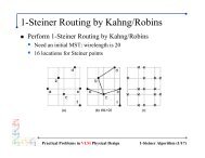
Defect Etching<br />
� Certain etches attack defective regions allowing defect<br />
identification (etch recipes given at end <strong>of</strong> notes)<br />
D.C. Miller and G.A. Rozgonyi, “Defect Characterization by Etching, Optical Microscopy, and X-Ray Topography,”<br />
in Handbook on Semiconductors 3 (S.P. Keller, ed.) North-Holland, Amsterdam, 1980, 217-246. ASTM Standards<br />
F47 and F26, 1997 Annual Book <strong>of</strong> ASTM Standards, Am. Soc. Test. Mat., West Conshohocken, PA, 1997.<br />
<strong>ECE</strong> 4813 Dr. Alan Doolittle
Defect Etching<br />
� Different etches attack defective regions differently<br />
� Can be accentuated through copper decoration<br />
A Defects - Interstitials<br />
Secco Wright A Defects: HF+HNO 3 A Defects: HF+HNO 3+H 3PO 4<br />
D Defects - Vacancies<br />
1.25 mm<br />
Secco Wright HF+HNO 3 HF+HNO 3+H 3PO 4<br />
Micrographs courtesy <strong>of</strong> M.S. Kulkarni, MEMC (J. Electrochem. Soc. 149, G153, Feb. 2002)<br />
<strong>ECE</strong> 4813 Dr. Alan Doolittle
Defect Etch References<br />
[1] E. Sirtl and A. Adler, “Chromic Acid-Hydr<strong>of</strong>luoric Acid as Specific Reagents for the<br />
Development <strong>of</strong> Etching Pits in Silicon,” Z. Metallkd. 52, 529-534, Aug. 1961.<br />
[2] W.C. Dash, “Copper Precipitation on Dislocations in Silicon,” J. Appl. Phys. 27, 1193-1195,<br />
Oct. 1956; “Evidence <strong>of</strong> Dislocation Jogs in Deformed Silicon,” J. Appl. Phys. 29, 705-709,<br />
April 1958.<br />
[3] F. Secco d'Aragona, “Dislocation Etch for (100) Planes in Silicon,” J. Electrochem. Soc. 119,<br />
948-951, July 1972.<br />
[4] D.G. Schimmel, “Defect Etch for Silicon Ingot Evaluation,” J. Electrochem. Soc. 126,<br />
479-483, March 1979; D.G. Schimmel and M.J. Elkind, “An Examination <strong>of</strong> the Chemical<br />
Staining <strong>of</strong> Silicon,” J. Electrochem. Soc. 125, 152-155, Jan. 1978.<br />
[5] M.W. Jenkins, “A New Preferential Etch for Defects in Silicon Crystals,” J. Electrochem. Soc.<br />
124, 757-762, May 1977.<br />
[6] K.H. Yang,“An Etch for Delineation <strong>of</strong> Defects in Silicon,” J. Electrochem. Soc. 131, 1140-1145,<br />
May 1984.<br />
[7] H. Seiter, “Integrational Etching Methods,” in Semiconductor Silicon/1977 (H.R. Huff and E.<br />
Sirtl, eds.), Electrochem. Soc., Princeton, NJ, 1977, pp. 187-195.<br />
[8] K. Graff and P. Heim, “Chromium-Free Etch for Revealing and Distinguishing Metal<br />
Contamination Defects in Silicon,” J. Electrochem. Soc. 141, 2821-2825, Oct. 1994.<br />
[9] M. Ishii, R. Hirano, H. Kan and A Ito, “Etch Pit Observation <strong>of</strong> Very Thin {001}-GaAs Layer by<br />
Molten KOH,” Japan. J. Appl. Phys. 15, 645-650, April 1976; for a more detailed discussion <strong>of</strong><br />
GaAs Etching see D.J. Stirland and B.W. Straughan, “A Review <strong>of</strong> Etching and Defect<br />
Characterisation <strong>of</strong> Gallium Arsenide Substrate Material,” Thin Solid Films 31, 139-170, Jan.<br />
1976.<br />
[10] D.T.C. Huo, J.D. Wynn, M.Y. Fan and D.P. Witt, “InP Etch Pit Morphologies Revealed by Novel<br />
HCl-Based Etchants,” J. Electrochem. Soc. 136, 1804-1806, June 1989.<br />
<strong>ECE</strong> 4813 Dr. Alan Doolittle
Impurities or Defects<br />
� Shallow-level impurities (dopants) - measure optically<br />
� Photoluminescence<br />
� Photoelectron spectroscopy<br />
� Deep-level impurities (metals) - measure electrically<br />
� Deep level transient spectroscopy (DLTS)<br />
� Need to determine<br />
� Impurity density, N T<br />
� Impurity energy level, E T<br />
� Capture Cross section σ T<br />
Si<br />
Dopant<br />
Metal<br />
E T<br />
E c<br />
E v<br />
Shallow-level<br />
Impurities<br />
Deep-level<br />
Impurities<br />
<strong>ECE</strong> 4813 Dr. Alan Doolittle
Generation-Recombination<br />
� Consider a semiconductor with a deep-level impurity at<br />
energy E = E T<br />
� Electrons and holes can be captured and emitted<br />
� Capture is characterized by the capture coefficients c n & c p<br />
� c n = σ nv th where σ n is the capture cross section [cm 2 ] and v th is the<br />
thermal velocity <strong>of</strong> electrons. Similarly for holes.<br />
� Emission is characterized by emission rates e n and e p<br />
� The electron (n T) and hole (p T) occupation is also needed<br />
E<br />
n<br />
c n<br />
p T n T<br />
e n<br />
c p<br />
(a) (b) (c) (d)<br />
e p<br />
E C<br />
E T<br />
E V<br />
x<br />
n T + p T = N T<br />
<strong>ECE</strong> 4813 Dr. Alan Doolittle
Donors and Acceptors<br />
� G-R centers can be donors or acceptors<br />
� The charge state is :<br />
Donor: Acceptor:<br />
"0" "+" "-" "0"<br />
<strong>ECE</strong> 4813 Dr. Alan Doolittle
Carrier Statistics<br />
� The change in electron and hole densities n and p is<br />
dn<br />
dt<br />
dp<br />
dt<br />
|<br />
G − R<br />
|<br />
G − R<br />
= ( b)<br />
− ( a)<br />
=<br />
= ( d)<br />
− ( c)<br />
=<br />
� The change in trap density is<br />
dn<br />
dt<br />
dp<br />
dt<br />
dn<br />
dt<br />
e<br />
e<br />
n<br />
p<br />
n<br />
T<br />
p<br />
T<br />
− c<br />
n<br />
− c<br />
p<br />
np<br />
T<br />
pn<br />
T | G −R<br />
= − = ( cnn<br />
+ ep<br />
)( NT<br />
− nT<br />
) − ( cpp<br />
+ en<br />
nT<br />
� This equation is difficult to solve because, in general, we<br />
do not know n and p<br />
T<br />
)<br />
E<br />
n<br />
c n<br />
p T n T<br />
e n<br />
c p<br />
e p<br />
(a) (b) (c) (d)<br />
E C<br />
E T<br />
E V<br />
<strong>ECE</strong> 4813 Dr. Alan Doolittle<br />
x
Carrier Statistics<br />
� Solving the dn T/dt equation gives<br />
n<br />
T<br />
( t)<br />
=<br />
n<br />
T<br />
( 0)<br />
exp( −t<br />
/ τ ) +<br />
e<br />
τ =<br />
e<br />
n<br />
n<br />
+ c<br />
( e<br />
+ c<br />
n<br />
p<br />
n<br />
+ c<br />
1<br />
n + e<br />
n + e<br />
p<br />
n<br />
n)<br />
N<br />
p<br />
+ c<br />
+ c<br />
p<br />
T<br />
p<br />
p<br />
p<br />
( 1−<br />
exp( −t<br />
/ τ ) )<br />
� Now consider an n-type semiconductor with<br />
electron capture and emission only<br />
n<br />
T<br />
cnn<br />
( t)<br />
= nT<br />
( 0)<br />
exp( −t<br />
/ τ1)<br />
+ NT<br />
( 1−<br />
exp( −t<br />
/ τ1)<br />
) ; τ1<br />
=<br />
e + c n<br />
emission<br />
n<br />
n<br />
capture<br />
e<br />
n<br />
1<br />
+ c<br />
n<br />
n<br />
<strong>ECE</strong> 4813 Dr. Alan Doolittle
Electron Emission<br />
� Simplifying Assumptions:<br />
�All G-R centers are occupied by electrons for t < 0<br />
�<strong>For</strong> t ≥ 0, electrons are emitted<br />
n<br />
T<br />
− t<br />
− t 1<br />
( t)<br />
≈ nT<br />
( 0)<br />
exp( ) ≈ NT<br />
exp( ); τ e =<br />
τ<br />
τ e<br />
n T (t)/N T<br />
1<br />
0.8<br />
0.6<br />
0.4<br />
0.2<br />
0<br />
e<br />
0 1 2<br />
t/τe 3 4<br />
e<br />
n<br />
<strong>ECE</strong> 4813 Dr. Alan Doolittle
Electron Capture<br />
� Simplifying Assumptions:<br />
n<br />
T<br />
�All G-R centers are empty <strong>of</strong> electrons for t < 0<br />
�<strong>For</strong> t ≥ 0, electrons are captured<br />
− t ⎛ − t ⎞ ⎛ − t ⎞ 1<br />
( t)<br />
= nT<br />
( 0)<br />
exp( ) + NT<br />
⎜1−<br />
exp( ) ⎟ ≈ NT<br />
⎜1−<br />
exp( ) ⎟;<br />
τ c =<br />
τ c ⎝ τ c ⎠ ⎝ τ c ⎠ cnn<br />
n T (t)/N T<br />
1<br />
0.8<br />
0.6<br />
0.4<br />
0.2<br />
0<br />
0 1 2<br />
t/τc 3 4<br />
<strong>ECE</strong> 4813 Dr. Alan Doolittle
Steady State<br />
� We have assumed that all G-R centers are either<br />
completely occupied by electrons or completely empty<br />
� From<br />
n<br />
T<br />
− t ( ep<br />
+ cnn)<br />
NT<br />
⎛ − t ⎞<br />
( t)<br />
= nT<br />
( 0)<br />
exp( ) +<br />
⎜1−<br />
exp( ) ⎟<br />
τ e + c n + e + c p ⎝ τ ⎠<br />
� <strong>For</strong> Steady state, t → ∞<br />
n<br />
T<br />
=<br />
e<br />
n<br />
n<br />
e<br />
+ c<br />
n<br />
p<br />
n<br />
+ c<br />
n<br />
n + e<br />
n<br />
p<br />
p<br />
+ c<br />
p<br />
p<br />
N<br />
p<br />
� <strong>For</strong> n ≈ p ≈ 0 in the space-charge region<br />
n<br />
T<br />
=<br />
e<br />
n<br />
e<br />
p<br />
+ e<br />
� <strong>For</strong> G-R centers in the lower half <strong>of</strong> the band gap, e n
Capacitance Transient<br />
� When carriers are captured or emitted, the charge<br />
changes with time<br />
� Can detect this by measuring current, capacitance, or<br />
charge<br />
� Capacitance is most commonly measured<br />
C<br />
=<br />
A<br />
qKsε<br />
0N<br />
2<br />
( V −V<br />
)<br />
� N scr is the total charge in the space-charge region<br />
including both dopants and defects<br />
+<br />
+<br />
+<br />
+<br />
-<br />
-<br />
N +<br />
D (Donor)<br />
bi<br />
n-Type<br />
N<br />
-<br />
T (Acceptor)<br />
scr<br />
N<br />
scr<br />
+ −<br />
= ND<br />
− NT<br />
<strong>ECE</strong> 4813 Dr. Alan Doolittle
Capacitance Emission Transient<br />
� The Schottky diode is zero biased<br />
� Assume all G-R centers are filled with electrons<br />
� The diode is reverse biased<br />
� Electrons are emitted from the G-R centers<br />
V=0<br />
W<br />
n-type<br />
N D<br />
n T<br />
V<br />
-V 1<br />
E C E F<br />
E T<br />
E V<br />
-V 1<br />
t<br />
W<br />
C<br />
C(V=0)<br />
-V 1<br />
W<br />
C0 ∆C0 0 t<br />
<strong>ECE</strong> 4813 Dr. Alan Doolittle
Capacitance Emission Transient<br />
C<br />
( t )<br />
=<br />
A<br />
qK<br />
0(<br />
ND<br />
− nT<br />
( t ) )<br />
( V −V<br />
)<br />
� Usually N T
Capacitance Transient<br />
� What information is contained in the capacitance<br />
transient?<br />
� In thermal equilibrium dn/dt = dp/dt =0<br />
n<br />
0<br />
=<br />
n<br />
i<br />
e −<br />
n0nT<br />
0 = cn0n0<br />
pT<br />
0 = cn0n0<br />
( NT<br />
nT<br />
0<br />
( E − E )<br />
⎛ F i ⎞<br />
exp⎜ ⎟;<br />
nT<br />
0<br />
⎝ kT ⎠<br />
=<br />
1+<br />
exp<br />
� <strong>For</strong> E F = E T, n T0 = N T/2 = p T0, n = n 1<br />
e<br />
n0<br />
=<br />
c<br />
n0<br />
n<br />
1<br />
=<br />
c<br />
n0<br />
n<br />
⎛ ET<br />
− E<br />
⎜<br />
⎝ kT<br />
⎞<br />
⎟<br />
⎠<br />
=<br />
c<br />
i<br />
i exp n0<br />
N<br />
)<br />
N<br />
( ( E − E ) kT )<br />
C<br />
T<br />
T<br />
F<br />
⎛ − ( EC<br />
− E<br />
exp⎜<br />
⎝ kT<br />
T<br />
) ⎞<br />
⎟<br />
⎠<br />
=N Tf(E T)<br />
<strong>ECE</strong> 4813 Dr. Alan Doolittle
Capacitance Transient<br />
� Then assume non-equilibrium emission and capture rates<br />
remain equal to their equilibrium values:<br />
e n0 = e n and e p0 = e p<br />
n<br />
1<br />
=<br />
N<br />
1 c e n c en = n p = p<br />
⎛ EC<br />
− E<br />
⎜ −<br />
⎝ kT<br />
⎞<br />
⎟;<br />
⎠<br />
; p<br />
= N<br />
N1 and p1 describe the trap occupancy for electrons and holes<br />
p<br />
T<br />
C exp 1<br />
V<br />
1<br />
⎛ ET<br />
− E<br />
exp⎜<br />
−<br />
⎝ kT<br />
V<br />
⎞<br />
⎟<br />
⎠<br />
<strong>ECE</strong> 4813 Dr. Alan Doolittle
Capacitance Transient<br />
� Then assume non-equilibrium emission and capture rates<br />
remain equal to their equilibrium values:<br />
τ<br />
τ<br />
=<br />
e<br />
exp<br />
exp c =<br />
σ K T<br />
=<br />
e<br />
=<br />
1<br />
=<br />
e<br />
n<br />
exp<br />
n<br />
exp<br />
1<br />
=<br />
c n<br />
( ( E − E ) kT )<br />
( ( E − E ) kT )<br />
1<br />
c<br />
σ ν<br />
n<br />
1/<br />
2<br />
1<br />
N<br />
K<br />
( ( E − E ) kT )<br />
c<br />
n<br />
n<br />
th<br />
σ γ T<br />
n<br />
T<br />
T<br />
c<br />
2<br />
T<br />
2<br />
T<br />
3/<br />
2<br />
( ( E − E ) kT )<br />
c<br />
γ σ T<br />
n<br />
n<br />
T<br />
2<br />
…where K 1 and K 2 are temporary<br />
constants used in the derivation<br />
…where γn = K1K2 =3.25x10²¹ (mn/mo) cm-2s-1K-2 is a constant derived from the<br />
temperature independent part <strong>of</strong> the<br />
thermal velocity and effective density <strong>of</strong><br />
states.<br />
3 2<br />
⎛ 2πm<br />
⎛ 3 ⎞<br />
nkT<br />
⎞ kT<br />
where N = 2⎜<br />
, =<br />
2 ⎟ ⎜<br />
⎟<br />
c<br />
ν th<br />
⎝ h ⎠ ⎝ mn<br />
⎠<br />
1 2<br />
<strong>ECE</strong> 4813 Dr. Alan Doolittle
Emission Time Constant<br />
τ e (s)<br />
10-11 10-9 10-7 10-5 10-3 10-1 101 103 105 τ<br />
e<br />
=<br />
exp<br />
( ( E − E ) kT )<br />
c<br />
σ γ T<br />
n<br />
n<br />
0 0.2 0.4 0.6 0.8 1<br />
T<br />
2<br />
T=200 K<br />
225 K<br />
300 K<br />
250 K 275 K<br />
γ n =1.07x10 21 cm -2 s -1 K -2<br />
E C -E T (eV)<br />
σ n =10 -15 cm 2<br />
One can normalize this temperature variation by plotting<br />
ln(T2τe) instead <strong>of</strong> ln(τe) <strong>ECE</strong> 4813 Dr. Alan Doolittle
Minority Carrier Emission<br />
� <strong>For</strong> majority carrier emission from acceptor impurities<br />
scr<br />
( t = 0)<br />
= ND<br />
− NT<br />
; Nscr<br />
( t → ∞)<br />
ND<br />
N =<br />
� <strong>For</strong> minority carrier emission from acceptor impurities<br />
scr<br />
( t = 0)<br />
= ND;<br />
Nscr<br />
( t → ∞)<br />
= ND<br />
NT<br />
N −<br />
C<br />
C 0<br />
0<br />
Nscr =ND exp(-t/τ )=exp(-e t)<br />
e n<br />
N scr =N D -N T<br />
exp(-t/τ e )=exp(-e p t)<br />
t<br />
N scr =N D<br />
Majority<br />
Carriers<br />
N scr =N D -N T<br />
Minority<br />
Carriers<br />
<strong>ECE</strong> 4813 Dr. Alan Doolittle
Deep-Level Transient Spectroscopy (DLTS)<br />
� DLTS is a method to automate the capacitance transient<br />
δC<br />
= C<br />
C<br />
( t )<br />
( t ) − C(<br />
t )<br />
1<br />
⎡ nT<br />
= C0<br />
⎢1−<br />
⎣ 2N<br />
2<br />
=<br />
C0nT<br />
2N<br />
( 0)<br />
D<br />
( 0)<br />
D<br />
⎛ − t ⎞⎤<br />
exp⎜<br />
⎟⎥<br />
⎝ τ e ⎠⎦<br />
� Measure C at t = t 1 and t = t 2, then subtract<br />
Capacitance (pF)<br />
4.9<br />
4.85<br />
4.8<br />
300 K<br />
280 K<br />
260 K<br />
240 K<br />
t T=200 K<br />
1 t2 4.75<br />
0 0.0005 0.001 0.0015 0.002<br />
Time (s)<br />
250 K<br />
220 K<br />
⎛ ⎛ − t<br />
⎜<br />
⎜exp⎜<br />
⎝ ⎝ τ e<br />
δC (pF)<br />
0<br />
-0.01<br />
-0.02<br />
2<br />
⎞ ⎛ − t<br />
⎟ − exp⎜<br />
⎠ ⎝ τ e<br />
1<br />
⎞⎞<br />
⎟<br />
⎟<br />
⎠⎠<br />
T 1<br />
-0.03<br />
t1 =5x10<br />
-0.04<br />
200 220 240 260 280 300<br />
-4 s<br />
t2 =10-3 s<br />
δCmax Temperature (K)<br />
<strong>ECE</strong> 4813 Dr. Alan Doolittle
δC<br />
= C<br />
( t ) − C(<br />
t )<br />
1<br />
2<br />
τ<br />
e<br />
=<br />
=<br />
DLTS<br />
C0nT<br />
2N<br />
exp<br />
( 0)<br />
D<br />
⎛ ⎛ − t<br />
⎜<br />
⎜exp⎜<br />
⎝ ⎝ τ e<br />
( ( E − E ) kT )<br />
⎞ ⎛ − t<br />
⎟ − exp⎜<br />
⎠ ⎝ τ e<br />
� Differentiate δC with respect to T, set equal to zero and<br />
solve for τ e<br />
e,<br />
max<br />
� Now we have τ e,max and T 1<br />
τ<br />
c<br />
σ γ T<br />
n<br />
n<br />
T<br />
2<br />
t2<br />
− t1<br />
=<br />
ln t<br />
( t )<br />
� Each DLTS temperature scan (peaks in spectra) result in<br />
only one emission time constant-temperature pair.<br />
Several such scans are needed to be plotted in an<br />
Arrhenius plot<br />
2<br />
1<br />
2<br />
1<br />
⎞⎞<br />
⎟<br />
⎟<br />
⎠⎠<br />
<strong>ECE</strong> 4813 Dr. Alan Doolittle
� DLTS plots are made for<br />
various t 1/t 2 ratios<br />
� Determine τ e,max and T 1 for<br />
each curve<br />
� Plot ln(τ e,max T 2 ) vs. 1/T<br />
τ T<br />
e<br />
2<br />
= exp<br />
( ( E − E ) kT )<br />
� Slope gives E c - E T and<br />
intercept gives σ n<br />
2 ( )<br />
c<br />
γ<br />
n<br />
σ<br />
n<br />
( E − E )<br />
T<br />
( γ )<br />
c T<br />
eT<br />
= − nσ<br />
n<br />
ln τ ln<br />
kT<br />
DLTS<br />
δC (F)<br />
0<br />
-1 10 -17<br />
-2 10 -17<br />
0.5 ms, 1 ms<br />
1 ms, 2 ms<br />
2 ms, 4 ms<br />
t1 =4 ms, t2 =8 ms<br />
-3 10-17 150 200 250 300 350 400<br />
ln(τ e T 2 )<br />
7<br />
6<br />
5<br />
4<br />
T (K)<br />
3<br />
0.002 0.003 0.004 0.005<br />
1/T (K -1 )<br />
<strong>ECE</strong> 4813 Dr. Alan Doolittle
� Since δC max ≠ ∆C e<br />
∆C<br />
δC<br />
DLTS<br />
2N<br />
( r −1)<br />
NT = 2ND<br />
e =<br />
C0<br />
max<br />
C0<br />
r<br />
D<br />
( 1−<br />
r )<br />
= −8ND<br />
C<br />
C 0<br />
t 1<br />
r<br />
δC max<br />
t 2<br />
∆C e<br />
t<br />
δC<br />
C<br />
max<br />
0<br />
for<br />
r<br />
=<br />
r = t 2/t 1<br />
2<br />
<strong>ECE</strong> 4813 Dr. Alan Doolittle
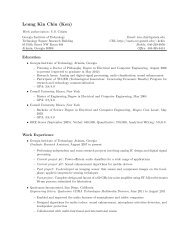
DLTS Example<br />
� Problem: BV CBO <strong>of</strong> BJT degraded from 1000 V to 500 V<br />
� BV CBO normal at T=77 K<br />
� Epi starting wafers were OK<br />
� Resistivity dropped after processing; 50 Ω-cm ⇒ 15 Ω-cm<br />
� Search for fast-diffusing deep donor impurity<br />
δC<br />
DLTS Rutherford Backscattering<br />
-150 -100 -50 T(°C)<br />
E C - 0.56 eV<br />
E C - 0.35 eV<br />
Selenium contamination from deteriorating rubber O-ring in sink<br />
RBS Yield<br />
Se<br />
Energy<br />
<strong>ECE</strong> 4813 Dr. Alan Doolittle
DLTS Variations<br />
� The primary task <strong>of</strong> a DLTS system is determine ∆C, τ e<br />
vs T so as to extract N T, E T, and σ n.<br />
� This goal can be performed by direct digitation and analysis <strong>of</strong> the<br />
capacitance transient without going to the extremes <strong>of</strong> using analog signal<br />
processing techniques →DSP or numerical fitting<br />
� Trade <strong>of</strong>fs in trap sensitivity versus trap energy resolution exist for all<br />
techniques and it can be shown that energy resolution improves as<br />
temperature decreases*<br />
� Analog signal processing techniques (Boxcar, Lockin and correlation<br />
methods) can have extremely good trap sensitivity (detection <strong>of</strong> N T
DLTS Variations<br />
� σ n can measured directly by making the filling pulse<br />
short enough in time (less than the capture time<br />
constant) to result in incomplete filling <strong>of</strong> the trap states<br />
(i.e. t f
DLTS Variations<br />
� A seemingly small but important point:<br />
� All thermal measurements (DLTS, Hall, etc…) measure<br />
the change in Gibbs free energy <strong>of</strong> a defect.<br />
G=H-TS so ∆G=∆H-T∆S<br />
…where H is enthalpy and S is entropy<br />
� All optical measurements (i.e. ones where an initial to<br />
final state transition occurs) are not effected by entropy<br />
(other than line broadening) making them measure ∆H<br />
not ∆G.<br />
� Electrically determined activation energies are almost<br />
always lower than optically determined activation<br />
energies by a factor ∆S<br />
� See Appendix 5.1 and references therein for details.<br />
<strong>ECE</strong> 4813 Dr. Alan Doolittle
Review Questions<br />
� Name some common defects in Si wafers.<br />
� What do metallic impurities do in Si devices?<br />
� Name some defect sources.<br />
� What are point defects? Name three point defects.<br />
� Name a line defect, an area defect, and a volume defect.<br />
� How do oxidation-induced stacking faults originate?<br />
� What determines the capacitance transient?<br />
� Where does the energy for thermal emission come from?<br />
� Why do minority and majority carrier emission have<br />
opposite behavior?<br />
� What is deep level transient spectroscopy (DLTS)?<br />
� What parameters can be determined with DLTS?<br />
<strong>ECE</strong> 4813 Dr. Alan Doolittle