Tolls on the New Jersey Turnpike - Distance Education @ NCSSM
Tolls on the New Jersey Turnpike - Distance Education @ NCSSM
Tolls on the New Jersey Turnpike - Distance Education @ NCSSM
You also want an ePaper? Increase the reach of your titles
YUMPU automatically turns print PDFs into web optimized ePapers that Google loves.
2003-2004<br />
Student Handout<br />
<strong>New</strong> <strong>Jersey</strong> <strong>Turnpike</strong>: A Toll Road<br />
Name______________<br />
A F M<br />
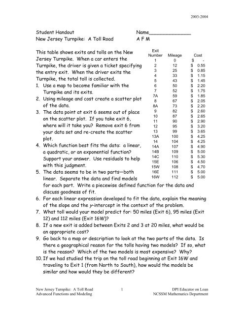
This table shows exits and tolls <strong>on</strong> <strong>the</strong> <strong>New</strong> Exit<br />
Number Mileage Cost<br />
<strong>Jersey</strong> <strong>Turnpike</strong>. When a car enters <strong>the</strong><br />
1 0 $ -<br />
<strong>Turnpike</strong>, <strong>the</strong> driver is given a ticket specifying 2 12 $ 0.55<br />
<strong>the</strong> entry exit. When <strong>the</strong> driver exits <strong>the</strong><br />
3 25 $ 0.85<br />
4 33 $ 1.15<br />
<strong>Turnpike</strong>, <strong>the</strong> total toll is collected.<br />
5 43 $ 1.45<br />
1. Use a map to become familiar with <strong>the</strong><br />
6 50 $ 2.20<br />
<strong>Turnpike</strong> and its exits.<br />
7 52 $ 1.75<br />
7A 59 $ 1.85<br />
2. Using mileage and cost create a scatter plot 8 67 $ 2.05<br />
of <strong>the</strong> data.<br />
8A 73 $ 2.20<br />
3. The data point at exit 6 seems out of place 9 82 $ 2.60<br />
10 87 $ 2.65<br />
<strong>on</strong> <strong>the</strong> scatter plot. If you take exit 6,<br />
11 90 $ 2.90<br />
where will it take you? Remove exit 6 from 12 95 $ 3.20<br />
your data set and re-create <strong>the</strong> scatter<br />
13 99 $ 3.65<br />
13A 100 $ 4.25<br />
plot.<br />
14 104 $ 4.25<br />
4. Which functi<strong>on</strong> best fits <strong>the</strong> data: a linear, 14A 107 $ 4.90<br />
a quadratic, or an exp<strong>on</strong>ential functi<strong>on</strong>?<br />
14B 109 $ 5.00<br />
14C 110 $ 5.30<br />
Support your answer. Use residuals to help<br />
15E 106 $ 4.50<br />
with this judgment.<br />
15W 108 $ 4.70<br />
5. The data seems to be in two parts—both 16E 111 $ 5.00<br />
linear. Separate <strong>the</strong> data and find models 16W 112 $ 5.00<br />
for each part. Write a piecewise defined functi<strong>on</strong> for <strong>the</strong> data and<br />
discuss goodness of fit.<br />
6. For each linear expressi<strong>on</strong> developed to fit <strong>the</strong> data, explain <strong>the</strong> meaning<br />
of <strong>the</strong> slope and <strong>the</strong> y-intercept in <strong>the</strong> c<strong>on</strong>text of <strong>the</strong> problem.<br />
7. What toll would your model predict for: 50 miles (Exit 6), 95 miles (Exit<br />
12) and 112 miles (Exit 16W)?<br />
8. If a new exit is added between Exits 2 and 3 at 20 miles, what would be<br />
an appropriate cost?<br />
9. Go back to a map or descripti<strong>on</strong> to look at <strong>the</strong> two parts of <strong>the</strong> data. Is<br />
<strong>the</strong>re a geographical reas<strong>on</strong> for <strong>the</strong> tolls having two models? If so, what<br />
is <strong>the</strong> reas<strong>on</strong>? Which of <strong>the</strong> two models is most expensive? Why?<br />
10. If we had studied <strong>the</strong> trip <strong>on</strong> <strong>the</strong> toll road beginning at Exit 16W and<br />
traveling to Exit 1 (from North to South), how would <strong>the</strong> models be<br />
similar and how would <strong>the</strong>y be different?<br />
<strong>New</strong> <strong>Jersey</strong> <strong>Turnpike</strong>: A Toll Road 1 DPI Educator <strong>on</strong> Loan<br />
Advanced Functi<strong>on</strong>s and Modeling<br />
<strong>NCSSM</strong> Ma<strong>the</strong>matics Department
2003-2004<br />
<str<strong>on</strong>g>Tolls</str<strong>on</strong>g> <strong>on</strong> <strong>the</strong> <strong>New</strong> <strong>Jersey</strong> <strong>Turnpike</strong><br />
Advanced Functi<strong>on</strong>s and Modeling<br />
Students develop a model for <strong>the</strong> toll structure of <strong>the</strong> <strong>New</strong> <strong>Jersey</strong> turnpike using a<br />
piecewise defined linear functi<strong>on</strong> developed using data analysis. This problem is based<br />
<strong>on</strong> work d<strong>on</strong>e by John A. Goebel for his Algebra 2 class at Durham Academy in 2003.<br />
Goals Addressed in <strong>the</strong> Less<strong>on</strong>:<br />
1. Create and use calculator-generated models of a linear functi<strong>on</strong> of bivariate data to<br />
solve problems. (1.01)<br />
a. Interpret <strong>the</strong> c<strong>on</strong>stants and coefficients in <strong>the</strong> c<strong>on</strong>text of <strong>the</strong> data.<br />
b. Check models for goodness of fit; use <strong>the</strong> most appropriate model to draw<br />
c<strong>on</strong>clusi<strong>on</strong>s and make predicti<strong>on</strong>s.<br />
2. Use piecewise-defined functi<strong>on</strong>s to model and solve problems; justify results. (2.02)<br />
a. Solve using tables, graphs, and algebraic properties.<br />
b. Interpret <strong>the</strong> c<strong>on</strong>stants and coefficients in <strong>the</strong> c<strong>on</strong>text of <strong>the</strong> problem.<br />
Materials Needed:<br />
1. Copy of <strong>the</strong> student handout for each student.<br />
2. Graphing calculator for each student.<br />
3. Graph paper.<br />
4. Access to <strong>the</strong> internet (if possible).<br />
5. Map of <strong>New</strong> <strong>Jersey</strong> or web link to <strong>New</strong> <strong>Jersey</strong> map.<br />
Activity One:<br />
The goal of this activity is to develop interest in <strong>the</strong> issue of toll roads—how do <strong>the</strong>y<br />
work, what do <strong>the</strong>y look like, why <strong>the</strong>y exist? We want <strong>the</strong> students to know something<br />
about <strong>the</strong> <strong>New</strong> <strong>Jersey</strong> <strong>Turnpike</strong> since <strong>the</strong> data in this problem is from <strong>the</strong>re. Several<br />
particular exits will be of interest so students need a way to determine where an exit takes<br />
<strong>the</strong>m. Some avenues to help students get acquainted are listed below.<br />
• Look at maps of <strong>New</strong> <strong>Jersey</strong><br />
• Go to http://www.state.nj.us/turnpike/nj-vcenter-maps.htm to view maps of <strong>the</strong><br />
<strong>New</strong> <strong>Jersey</strong> <strong>Turnpike</strong>.<br />
• A list of <strong>the</strong> interchanges and <strong>the</strong>ir locati<strong>on</strong>s can be found at<br />
http://www.c<strong>on</strong>trib.andrew.cmu.edu/~mn2n/tollroads.html.<br />
• A “road sign” tour is available at http://web.mit.edu/spui/www/freeway/njtp.html<br />
• There is a discussi<strong>on</strong> of <strong>the</strong> issues of toll roads at<br />
http://www.worldbank.org/transport/roads/toll_rds.htm#opti<strong>on</strong>s. Discuss <strong>the</strong><br />
purpose and <strong>the</strong> mechanics of toll roads.<br />
• A web site with a number of cameras <strong>on</strong> different parts of <strong>the</strong> <strong>New</strong> <strong>Jersey</strong><br />
<strong>Turnpike</strong> can be seen at<br />
http://newyork.metrocommute.com/video/newyork/indexNJTpke.html.<br />
Activity Two:<br />
The following data show <strong>the</strong> exit number, mileage (from first exit) and toll for <strong>the</strong> <strong>New</strong><br />
<strong>Jersey</strong> <strong>Turnpike</strong>. These data are for peak hours using an E-Z Pass. The E-Z Pass is an<br />
<strong>New</strong> <strong>Jersey</strong> <strong>Turnpike</strong>: A Toll Road 2 DPI Educator <strong>on</strong> Loan<br />
Advanced Functi<strong>on</strong>s and Modeling<br />
<strong>NCSSM</strong> Ma<strong>the</strong>matics Department
2003-2004<br />
electr<strong>on</strong>ic system that deducts tolls from a pre-established account. More informati<strong>on</strong> <strong>on</strong><br />
this pass is at http://www.state.nj.us/turnpike/nj-ezpass.htm.)<br />
1. Create a scatter plot of <strong>the</strong> data showing cost<br />
versus mileage.<br />
Exit<br />
Number Mileage Cost<br />
1 0 $ -<br />
2 12 $ 0.55<br />
3 25 $ 0.85<br />
4 33 $ 1.15<br />
5 43 $ 1.45<br />
6 50 $ 2.20<br />
7 52 $ 1.75<br />
7A 59 $ 1.85<br />
8 67 $ 2.05<br />
8A 73 $ 2.20<br />
9 82 $ 2.60<br />
10 87 $ 2.65<br />
11 90 $ 2.90<br />
12 95 $ 3.20<br />
13 99 $ 3.65<br />
13A 100 $ 4.25<br />
14 104 $ 4.25<br />
14A 107 $ 4.90<br />
14B 109 $ 5.00<br />
14C 110 $ 5.30<br />
15E 106 $ 4.50<br />
15W 108 $ 4.70<br />
16E 111 $ 5.00<br />
16W 112 $ 5.00<br />
Notice <strong>the</strong> point associated with exit 6 does not seem to fit <strong>the</strong> trend around it. Delete<br />
that point and rec<strong>on</strong>sider <strong>the</strong> data. Exit 6 takes a driver to <strong>the</strong> Pennsylvania <strong>Turnpike</strong>.<br />
4. Fit this data with a linear, quadratic, and exp<strong>on</strong>ential model. Discuss goodness of fit<br />
for each model. Which model is best?<br />
Note <strong>on</strong> Goodness of Fit: We will explore goodness of fit through residuals. A residual<br />
is defined as <strong>the</strong> vertical distance between a data point and <strong>the</strong> model describing <strong>the</strong> data.<br />
The value of a residual is calculated using <strong>the</strong> following formula<br />
For a given x data<br />
, <strong>the</strong> residual = ydata<br />
− ymodel<br />
.<br />
<strong>New</strong> <strong>Jersey</strong> <strong>Turnpike</strong>: A Toll Road 3 DPI Educator <strong>on</strong> Loan<br />
Advanced Functi<strong>on</strong>s and Modeling<br />
<strong>NCSSM</strong> Ma<strong>the</strong>matics Department
2003-2004<br />
The values of <strong>the</strong> residuals are found <strong>on</strong> <strong>the</strong> calculator using <strong>the</strong> lists. Given <strong>the</strong> x-values<br />
of <strong>the</strong> data in list L1, <strong>the</strong> y-values of <strong>the</strong> data in L2 and <strong>the</strong> model for <strong>the</strong> data in Y1, go to<br />
<strong>the</strong> top of L3 and type L3= L2−<br />
Y1( L1)<br />
A residual plot is created by plotting <strong>the</strong> ordered pair:( x , data<br />
residual ) . The residual plot<br />
should <strong>on</strong>ly show noise and should have no pattern. O<strong>the</strong>rwise, <strong>the</strong> model used may not<br />
be <strong>the</strong> best model for that data.<br />
Linear Model:<br />
y = 0.0473x −0.666<br />
where x = mileage and y = cost of toll.<br />
On <strong>the</strong> left, <strong>the</strong> linear model is shown below superimposed over <strong>the</strong> data. The residuals<br />
verify that this model is not a satisfactory <strong>on</strong>e. The residuals are shown in <strong>the</strong> middle<br />
graph and its window is <strong>on</strong> <strong>the</strong> far right.<br />
Quadratic Model:<br />
2<br />
y = 0.0049x − 0.02x + 1.07 where x = mileage and y = cost of toll.<br />
On <strong>the</strong> left, <strong>the</strong> quadratic model is shown below superimposed over <strong>the</strong> data. The<br />
residuals verify that this model is again not satisfactory (seems a bit better than <strong>the</strong> line).<br />
The residuals have a definite pattern which verifies <strong>the</strong> c<strong>on</strong>cern with <strong>the</strong> model.<br />
x<br />
Exp<strong>on</strong>ential Model: y = 0.5243 ⋅(1.0205)<br />
x = mileage and y = cost of toll.<br />
<strong>New</strong> <strong>Jersey</strong> <strong>Turnpike</strong>: A Toll Road 4 DPI Educator <strong>on</strong> Loan<br />
Advanced Functi<strong>on</strong>s and Modeling<br />
<strong>NCSSM</strong> Ma<strong>the</strong>matics Department
2003-2004<br />
On <strong>the</strong> left, <strong>the</strong> exp<strong>on</strong>ential model appears to fit <strong>the</strong> data; however, <strong>the</strong> residuals (shown<br />
in <strong>the</strong> middle) show a pattern. Thus, <strong>the</strong> exp<strong>on</strong>ential is also not a good model for this<br />
data. This fit is very similar to that of <strong>the</strong> quadratic functi<strong>on</strong>.<br />
As we look at <strong>the</strong>se three possible models, <strong>the</strong> exp<strong>on</strong>ential has residuals that are a bit<br />
smaller than those of <strong>the</strong> quadratic functi<strong>on</strong>, but a clear pattern is still visible in every<br />
residual plot. We need to c<strong>on</strong>sider o<strong>the</strong>r models.<br />
5. Separate <strong>the</strong> data into two parts. This will depend <strong>on</strong> how <strong>the</strong> student sees <strong>the</strong> data.<br />
For <strong>the</strong> purpose of producing a soluti<strong>on</strong>, we will break <strong>the</strong> data at exit 12 which is at<br />
95 miles. The point associated with exit 12 will be included in both data sets for <strong>the</strong><br />
purpose of fitting <strong>the</strong> line. When we write <strong>the</strong> model, <strong>the</strong> point at 95 miles must go<br />
with <strong>on</strong>ly <strong>on</strong>e part of <strong>the</strong> piecewise functi<strong>on</strong>.<br />
Students may select different breaking points and not choose to include <strong>the</strong> point in both<br />
sets. Hence, <strong>the</strong>re are many answers. This is <strong>on</strong>e example.<br />
For exits 1 through 12 or 0≤<br />
x ≤95, <strong>the</strong> regressi<strong>on</strong> line (using LinReg from <strong>the</strong> Stat Calc<br />
menu) is y = 0.0302x+ 0.1249 where x =<strong>the</strong> number of miles from exit 1 and y = <strong>the</strong><br />
cost of <strong>the</strong> toll when you exit. The line is shown superimposed over <strong>the</strong> data followed by<br />
<strong>the</strong> residual plot associated with this linear fit.<br />
<strong>New</strong> <strong>Jersey</strong> <strong>Turnpike</strong>: A Toll Road 5 DPI Educator <strong>on</strong> Loan<br />
Advanced Functi<strong>on</strong>s and Modeling<br />
<strong>NCSSM</strong> Ma<strong>the</strong>matics Department
2003-2004<br />
The residual plot shows that <strong>the</strong> line fits <strong>the</strong> beginning points best. The residuals show a<br />
fairly random shape as well as <strong>the</strong> value of <strong>the</strong> residuals is small which is shown by <strong>the</strong> y-<br />
values of <strong>the</strong> window.<br />
The sec<strong>on</strong>d part of <strong>the</strong> data for 95 ≤ x ≤ 112 or exits 12 through 16W is fit by <strong>the</strong><br />
regressi<strong>on</strong> line y = 0.1117x−7.2652<br />
where x = <strong>the</strong> number of miles from exit 1 and<br />
y = <strong>the</strong> cost of <strong>the</strong> toll when you exit. The line is shown superimposed over <strong>the</strong> data<br />
followed by <strong>the</strong> residual plot associated with this linear fit.<br />
This residual plot shows a very scattered set of points and reflects that <strong>the</strong> line is a good<br />
model for this data.<br />
The middle screen below shows <strong>the</strong> creati<strong>on</strong> of a piecewise functi<strong>on</strong> <strong>on</strong> <strong>the</strong> calculator.<br />
Find Y1 and Y2 <strong>on</strong> <strong>the</strong> VARS menu and <strong>the</strong> inequalities under TEST. A scatter plot of<br />
<strong>the</strong> full data set with <strong>the</strong> two lines superimposed over <strong>the</strong> data is shown.<br />
<strong>New</strong> <strong>Jersey</strong> <strong>Turnpike</strong>: A Toll Road 6 DPI Educator <strong>on</strong> Loan<br />
Advanced Functi<strong>on</strong>s and Modeling<br />
<strong>NCSSM</strong> Ma<strong>the</strong>matics Department
2003-2004<br />
The slopes and y-intercepts have meaning to <strong>the</strong> NJ <strong>Turnpike</strong>.<br />
• For <strong>the</strong> functi<strong>on</strong> y = 0.0302x+ 0.1249 where x =<strong>the</strong> number of miles from exit 1<br />
and y = <strong>the</strong> cost of <strong>the</strong> toll when you exit. This functi<strong>on</strong> represents exits 1<br />
through 12 or 0 ≤ x ≤95. The slope of 0.0302 measures <strong>the</strong> cost in dollars per<br />
mile <strong>on</strong> <strong>Turnpike</strong> for <strong>the</strong>se exits. More generally, <strong>the</strong> slope represents a cost of 3<br />
cents per mile. The y-intercept 0.1249 measures <strong>the</strong> initial cost in dollars for just<br />
entering <strong>the</strong> <strong>Turnpike</strong>.<br />
• For <strong>the</strong> functi<strong>on</strong> y = 0.1117x−7.2652<br />
which represents 95 ≤ x ≤ 112 or exits 12<br />
through 16W, <strong>the</strong> slope 0.1117 measures cost in dollars per mile. More simply, it<br />
costs 11 cents per mile to travel between exits 12 and 16W. The y-intercept is not<br />
really meaningful since x cannot be 0.<br />
⎧0.0302x+ 0.1249,0 ≤ x≤95<br />
Use <strong>the</strong> functi<strong>on</strong> tx ( ) = ⎨<br />
to find values of tolls.<br />
⎩0.1117x− 7.2652,95 < x≤112<br />
• At x = 50 , <strong>the</strong> model produces a toll of $1.64. At Exit 6, <strong>the</strong> toll is $2.20.<br />
• At x = 95, <strong>the</strong> model predicts a toll of $2.99. At Exit 12, <strong>the</strong> toll is $3.20.<br />
• At x =112 , <strong>the</strong> model predicts a toll of $5.24. At Exit 16W, <strong>the</strong> toll is $5.00.<br />
• If a new exit is added at x = 20 , <strong>the</strong> model predicts a toll of $0.72. For ease it<br />
would be changed to $0.75.<br />
9. A review of <strong>the</strong> map shows that <strong>on</strong>ce we pass Exit 12, <strong>the</strong> NJ <strong>Turnpike</strong> travels<br />
through a dense populati<strong>on</strong> area near <strong>New</strong> York City. The cost per mile greatly<br />
increases but also <strong>the</strong> cost of <strong>the</strong> turnpike does as well. There will have to be<br />
more lanes and more repairs and changes in <strong>the</strong> turnpike since it serves some<br />
many more people. Clearly, <strong>the</strong> most expensive travel is from exits 12 through<br />
16W.<br />
Possible Extensi<strong>on</strong><br />
Once this problem has been explored, students could develop a toll system for I-95 in<br />
North Carolina. To complete this task, students would need maps with I-95 exits and<br />
distances shown. There have been news articles with informati<strong>on</strong> about major goals. For<br />
example, follow <strong>the</strong> link to http://www.newsobserver.com/fr<strong>on</strong>t/digest/story/3025530p-<br />
2771057c.html. Perhaps as students produce <strong>the</strong>ir toll system, <strong>the</strong>y can work to have<br />
each car that travels <strong>the</strong> full length of I-95 in North Carolina pay a total of $18, while<br />
establishing toll booths as <strong>the</strong>y exit I-95 at certain exits.<br />
<strong>New</strong> <strong>Jersey</strong> <strong>Turnpike</strong>: A Toll Road 7 DPI Educator <strong>on</strong> Loan<br />
Advanced Functi<strong>on</strong>s and Modeling<br />
<strong>NCSSM</strong> Ma<strong>the</strong>matics Department


