Neutrinos from supernovae and failed supernovae
Neutrinos from supernovae and failed supernovae
Neutrinos from supernovae and failed supernovae

Create successful ePaper yourself
Turn your PDF publications into a flip-book with our unique Google optimized e-Paper software.
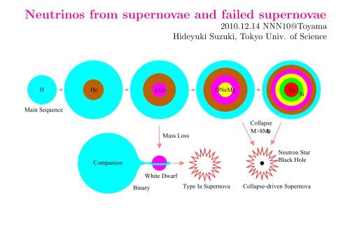
<strong>Neutrinos</strong> <strong>from</strong> <strong>supernovae</strong> <strong>and</strong> <strong>failed</strong> <strong>supernovae</strong><br />
2010.12.14 NNN10@Toyama<br />
Hideyuki Suzuki, Tokyo Univ. of Science<br />
H<br />
He CO ONeMg Fe Si<br />
Main Sequence<br />
Mass Loss<br />
Collapse<br />
M>8M<br />
Companion<br />
Neutron Star<br />
Black Hole<br />
Binary<br />
White Dwarf<br />
Type Ia Supernova<br />
Collapse-driven Supernova
1 Collapse-Driven Supernova Explosion<br />
SN Core (T ∼ 10MeV, ρ > ∼ 10 14 g/cm 3 )<br />
• τ weak ≪ τ dyn Neutrino Trapping<br />
⇒ <strong>Neutrinos</strong> are also in thermal equilibrium <strong>and</strong> in chemical equilibrium<br />
n ν ∼ n γ ∼ n e<br />
• mean free path length λ ν ≫ λ γ , λ e , λ N<br />
⇒ <strong>Neutrinos</strong> carry the energy <strong>and</strong> drive the evolution of the core<br />
⇒ SN core can be seen by neutrinos (neutrinosphere)<br />
SN as a neutrino source<br />
• source of all species (ν e ,¯ν e ,ν µ ,¯ν µ ,ν τ ,¯ν τ )<br />
• T < O(100MeV) = m µ ⇒ n e −<br />
≫ n µ , n τ : ν x ≡ ν µ , ¯ν µ , ν τ , ¯ν τ<br />
• ∫ L ν dt ∼ O(10 53 )erg ∼ 10 4 L ν⊙ τ ⊙ ∼ 10 2 L γ⊙ τ ⊙<br />
τ ∼ O(10)sec, d > O(10 18 )cm<br />
• Spectral difference: hierarchy of average energy(O(10)MeV)<br />
σ νe > σ¯νe > σ νx ⇒ 〈ω νe 〉
H<br />
He<br />
CO<br />
ONeMg<br />
Si<br />
νe<br />
Fe<br />
Fe core<br />
9−10<br />
ρ 3<br />
c =10 g/cm<br />
<strong>Neutrinos</strong>phere<br />
11<br />
ρ >10 g/cm<br />
c<br />
3<br />
ν trapping (ρ > 10 10 − 10 12 g/cm 3 )<br />
ν e <strong>from</strong> e − A −→ ν e A ′ <strong>and</strong> e − p −→ ν e n<br />
main opacity source: coherent scattering ν e A −→ ν e A<br />
cross section σ ∝ A 2 ων: 2 λ νA < λ νN<br />
(ν wave length ¯hc<br />
E<br />
E ν<br />
∼ 20fm( ν<br />
10MeV )−1 ≫ nuclear size 1.2A 1 3 fm ∼ 5fm( A 56 ) 1 3 )<br />
collapse<br />
σ∼E^2<br />
increase<br />
opaque<br />
ν<br />
trapping<br />
ν<br />
degenerate<br />
µ(ν) increase<br />
coherent<br />
scattering<br />
nuclei survive<br />
e capture suppress<br />
not so n−rich<br />
Positive feedback (Sato 1975)
νeneutronization<br />
burst<br />
shock stall<br />
ν(all)<br />
ρ c<br />
bounce<br />
14<br />
>10 g/cm<br />
3<br />
Proto<br />
Neutron<br />
Star<br />
shock wave<br />
τ(collapse)~O(10−100)ms<br />
τ (neutronization burst)
Prompt explosion (Hillebr<strong>and</strong>t, Nomoto <strong>and</strong> Wolff 1984). M MS = 9M ⊙<br />
Failed Prompt explosion (Hillebr<strong>and</strong>t 1987). M MS = 20M ⊙
Wilson’s Delayed explosion model (Colgate 1989).
shock revival<br />
νwind<br />
PNS cooling<br />
ν heating<br />
Hot Bubble<br />
t(core exp.)=O(1)s<br />
τ(PNS cooling)=O(10)s<br />
Supernova<br />
Explosion<br />
Neutron Star<br />
t(SNE)=hours−day<br />
SN1987A<br />
Crab nebula (remnant of<br />
SN1054)
Classical Simulations<br />
Totani et al., 1998<br />
early phase: hierarchy of average energy<br />
late phase: n-rich matter interacts ¯ν e <strong>and</strong><br />
ν x almost equally. degeneracy prohibits<br />
ν e interactions, too.<br />
neutrinos <strong>from</strong> protoneutron star cooling phase<br />
(Suzuki 2002)
Energetics<br />
• ∆E G =<br />
(<br />
GM<br />
2<br />
core<br />
R Fe core<br />
− GM 2 core<br />
R NS<br />
)<br />
∼ O(10 53 )erg<br />
• E kin (obs.)∼O(10 51 )erg, E rad (obs.)∼O(10 49 )erg, E GW (sim.)∼O(10 51 )erg<br />
• rest O(10 53 )erg ∼ E ν<br />
cf. E ν (SNIa) < 10 49 erg<br />
ν e ’s <strong>from</strong> neutronization of all protons<br />
26 M Fe core<br />
〈E νe 〉 ∼ 1.2 · 10 52 erg M Fe core 〈E νe 〉<br />
m Fe<br />
1.4M ⊙ 10MeV ∼ O(0.1) × E ν tot<br />
=⇒ thermal ν ≫ neutronization ν e =⇒ ν e , ¯ν e , ν x : roughly equipartiton
Neutrino Transfer<br />
distibution function f νi (t, ⃗r, ⃗p ν ) (7 independent variables)<br />
∂f ν<br />
+ d⃗r ∂f ν<br />
∂t p dt p ∂⃗r + d⃗p (<br />
ν ∂f ν ∂fν<br />
=<br />
dt p ∂⃗p ν<br />
∂t p<br />
)ν int.<br />
• Spherically symmetric case:<br />
f νi (t, r, ω ν = p ν c, µ = cos θ) (4 independent variables)<br />
⇒ Fully general relativistic Boltzmann solver<br />
(Mezzacappa, Burrows, Janka, Sumiyoshi+Yamada > ∼ 2000)<br />
• Non-spherical case: 2D/3D ν transfer in progress<br />
Neutrino Interactions (minimal st<strong>and</strong>ard: Bruenn’85)<br />
e − p ←→ ν e n e + n ←→ ¯ν e p e − A −→ ν e A ′ e + A −→ ¯ν e A ′<br />
e − e + ←→ ν¯ν plasmon ←→ ν¯ν NN −→ NNν¯ν ν e¯ν e ←→ ν x¯ν x<br />
νN −→ νN νA −→ νA νe ± −→ νe ± νν ′ −→ νν ′
Equation of States (EOS) for high density matter (T ≠ 0)<br />
• Lattimer-Swesty 1991: FORTRAN code<br />
Liquid Drop model: K s = 180, 220, 375MeV, S v = 29.3MeV<br />
E/n ∼ −B + K s (1 − n/n s ) 2 /18 + S v (1 − 2Y e ) 2 + · · ·<br />
• Shen’s EOS table (Shen et al., 1998)<br />
RMF (n,p,σ, ρ, ω) with TM1 parameter set(g ρ , · · ·) ⇐ Nuclear data including<br />
unstable nuclei<br />
ρ B , n B , Y e , T , F , U, P , S, A, Z, M ∗ , X n , X p , X α , X A , µ n , µ p<br />
grids: wide range T = 0, 0.1 ∼ 100MeV ∆ log T = 0.1<br />
Y e = 0, 0.01 ∼ 0.56 ∆ log Y e = 0.025<br />
ρ B = 10 5.1 ∼ 10 15.4 g/cm 3 ∆ log ρ B = 0.1<br />
Extension with hyperons (Ishizuka, Ohnishi), quarks (Nakazato)
Modern Simulations<br />
Light ONeMg core + CO shell(1.38M ⊙ ): weak explosion (O(10 50 )erg)<br />
(Progenitor: Nomoto 8-10M ⊙ )<br />
ν-heating + nuclear reaction ⇒ weak explosion<br />
res (prompt explosions,<br />
ups (Fryer et al. 1999).<br />
ional<br />
Fig. 1. Mass trajectories for the simulation with the W&H EoS as a<br />
function of post-bounce time (t pb ). Also plotted: shock position (thick<br />
solid line starting at time zero <strong>and</strong> rising to the upper right corner),<br />
gain radius (thin dashed line), <strong>and</strong> neutrinospheres (ν e : thick solid;<br />
¯ν e : thick dashed;ν µ , ¯ν µ ,ν τ , ¯ν τ : thick dash-dotted). In addition, the<br />
composition interfaces are plotted with different bold, labelled lines:<br />
the inner boundaries of the O-Ne-Mg layer at∼0.77 M ⊙ , of the C-O<br />
layer at∼1.26 M ⊙ , <strong>and</strong> of the He layer at 1.3769 M ⊙ . The two dotted<br />
lines represent the mass shells where the mass spacing between<br />
the plotted trajectories changes. An equidistant spacing of 5×10 −2 M ⊙<br />
was chosen up to 1.3579M ⊙ , between that value <strong>and</strong> 1.3765M ⊙ it was<br />
1.3×10 −3 M ⊙ , <strong>and</strong> 8×10 −5 M ⊙ outside.<br />
Fig. 3. Velocity profiles as functions of radius for different postbounce<br />
times for the simulation with the W&H EoS. The insert shows<br />
the velocity profile vs. enclosed mass at the end of our simulation.<br />
Kitaura et al., AAp 450(2006)345<br />
(Mezzacappa’07: 11.2M ⊙ model explodes, too)
L [10 52 erg s -1 ]<br />
4<br />
3<br />
2<br />
1<br />
L/10<br />
Accretion Phase<br />
Cooling Phase<br />
ν e<br />
ν e<br />
ν µ/τ<br />
10 0<br />
10 -1<br />
0<br />
10 -2<br />
[MeV]<br />
12<br />
10<br />
10<br />
8<br />
5<br />
0 0.05 0.1 0.15 0.2 2 4 6 8<br />
4<br />
Time after bounce [s]<br />
Neutrino luminosities <strong>and</strong> average energies at infinity for 8.8M ⊙<br />
L. Hüdepohl et al., PRL104 (2010) 251101<br />
progenitor.
Phase transition into quark matter<br />
Luminosity [10 53 erg/s]<br />
1<br />
0<br />
Luminosity [10 53 erg/s]<br />
1<br />
0<br />
0.255 0.26 0.265<br />
Time after bounce [s]<br />
rms Energy [MeV]<br />
30<br />
25<br />
20<br />
15<br />
10<br />
0 0.1 0.2 0.3 0.4 0.5<br />
Time after bounce [s]<br />
FIG. 1: Neutrino luminosities <strong>and</strong> rms neutrino energies as<br />
functions of time after bounce, sampled at 500 km radius in<br />
the comoving frame, for a 10 M ⊙ progenitor star as modeled<br />
in [17]: ν e in solid (blue), ¯ν e in dashed (red), <strong>and</strong> ν µ/τ in<br />
dot-dashed (green). In contrast to the deleptonization burst<br />
just after bounce (t ∼ 5 ms) the second burst at t ∼ 257−261<br />
ms is associated with the QCD phase transition. The inset<br />
shows the second burst blown up.<br />
Dasgupta et al., PRD81 (2010) 103005<br />
The second shock wave merges the first shock wave leading to explosion.<br />
¯ν e > ν e in the second burst (protonization)
Modern simulations with GR 1D Boltzmann ν-transfer<br />
canonical models: no explosion<br />
Newton+O(v/c)<br />
Relativistic<br />
10 3 Time After Bounce [s]<br />
Radius [km]<br />
10 2<br />
10 1<br />
0 0.1 0.2 0.3 0.4 0.5<br />
NH 13M ⊙ , GR Boltzman, LS EOS+Si burning<br />
Liebendörfer et al., Phys.Rev. D63 (2001) 103004<br />
(astro-ph/0006418 v2) Fig.6<br />
10 4<br />
Fig. 1.—Trajectories of selected mass shells vs. time <strong>from</strong> the start of the<br />
simulation. The shells are equidistantly spaced in steps of 0.02 M ,, <strong>and</strong> the<br />
trajectories of the outer boundaries of the iron core (at 1.28 M ,) <strong>and</strong> of the<br />
silicon shell (at 1.77 M ,) are indicated by thick lines. The shock is formed<br />
at 211 ms. Its position is also marked by a thick line. The dashed curve shows<br />
the position of the gain radius.<br />
WW 15M ⊙ , M Fe = 1.28M ⊙ , NR Boltzmann<br />
(tangent-ray method), only ν e ,¯ν e , without<br />
e − e + ↔ ν ¯ν, LS EOS, Rampp et al., ApJ 539<br />
(2000) L33 Fig.1<br />
10 3<br />
radius [km]<br />
10 2<br />
10 1<br />
10 0<br />
0.0<br />
0.2<br />
0.4<br />
time [sec]<br />
15M ⊙ , Shen EOS, Sumiyoshi et al., 2005.<br />
0.6<br />
0.8<br />
1.0<br />
Fig. 5.—Radial position (in km) of selected mass shells as a function of<br />
time in our fiducial 11 M model.<br />
NR 1D Boltzmann ν-transfer, Thompson et al.,<br />
ApJ 592 (2003) 434 Fig.5
Comparison between Boltzmann solvers<br />
Fig. 5.—(a) Shock position as a function of time for model N13. The shock in VERTEX (thin line) propagates initially faster <strong>and</strong> nicely converges after its maximum<br />
expansion to the position of the shock in AGILE-BOLTZTRAN (thick line). (b) Neutrino luminosities <strong>and</strong> rms energies for model N13 are presented as functions of<br />
time. The values are sampled at a radius of 500 km in the comoving frame. The solid lines belong to electron neutrinos <strong>and</strong> the dashed lines to electron antineutrinos. The<br />
line width distinguishes between the results <strong>from</strong> AGILE-BOLTZTRAN <strong>and</strong> VERTEX in the same way as in (a). The luminosity peaks are nearly identical; the rms<br />
energies have the tendency to be larger in AGILE-BOLTZTRAN.<br />
Liebendörfer et al., ApJ620(2005)840 Fig.5
2 Failed <strong>supernovae</strong><br />
implicit GR hydrodynamics + Boltzmann ν transfer code<br />
Sumiyoshi, Yamada, Suzuki, Chiba PRL97(2006) 091101<br />
Fig. 1.—Radial trajectories of mass elements of the core of a 40 M star as a<br />
function of time after bounce in the SH model. The location of the shock wave is<br />
shown by a thick dashed line.<br />
Fig. 2.—Radial trajectories of mass elements of the core of a 40 M star as a<br />
function of time after bounce in the LS model. The location of the shock wave is<br />
shown by a thick dashed line.<br />
luminosity [erg/s]<br />
2x10 53 1<br />
0<br />
0.0<br />
0.5<br />
1.0<br />
1.5<br />
time after bounce [sec]<br />
luminosity [erg/s]<br />
2x10 53 1<br />
0<br />
0.0<br />
0.5<br />
1.0<br />
time after bounce [sec]<br />
Progenitor 40M ⊙ , left: Shen EOS, right: Lattimer-Swesty EOS 180<br />
1.5<br />
L ν increases due to<br />
matter accretion<br />
ν x < ν e , ¯ν e <strong>from</strong> accreted<br />
matter<br />
Burst duration time<br />
strongly depends on<br />
EOS!
(a)<br />
Luminosity [10 53 erg/s]<br />
rms Energy [MeV]<br />
6<br />
5<br />
4<br />
3<br />
2<br />
1<br />
0<br />
40<br />
35<br />
30<br />
25<br />
20<br />
15<br />
10<br />
5<br />
e Neutrino<br />
e Antineutrino<br />
µ/τ <strong>Neutrinos</strong><br />
0 0.2 0.4 0.6 0.8 1 1.2 1.4<br />
Time After Bounce [s]<br />
(b)<br />
0 0.2 0.4 0.6 0.8 1 1.2 1.4<br />
Time After Bounce [s]<br />
Figure 2. Luminosities <strong>and</strong> mean energies during the post bounce phase<br />
of a core collapse simulation of a 40 M ⊙ progenitor model <strong>from</strong><br />
Woosley <strong>and</strong> Weaver (1995). Comparing eos1 (thick lines) <strong>and</strong> eos2<br />
(thin lines).<br />
Fischer et al., 2008
Failed supernova neutrinos: expected observation by SK<br />
Nakazato et al., PRD78 (2008) 083014<br />
FIG. 5: Time-integrated spectra before the neutrino oscillation for models W40S (left) <strong>and</strong> W40L (right). Solid, dashed <strong>and</strong><br />
dot-dashed lines represent the spectra of νe, ¯νe <strong>and</strong> νx, respectively.<br />
FIG. 8: Time-integrated total event number of <strong>failed</strong> supernova neutrinos for the normal mass hierarchy (left) <strong>and</strong> the inverted<br />
mass hierarchy (right). Error bars represents the upper <strong>and</strong> lower limits owing to the different nadir angles. The upper <strong>and</strong><br />
lower sets represent models W40S <strong>and</strong> W40L, respectively.<br />
θ 13 dependence for W40S vs. W40L<br />
FIG. 9 (color online). Time-integrated spectra for the total event number of <strong>failed</strong> supernova neutrinos for the normal mass hierarchy<br />
with sin 2 13 ¼ 10 8 (upper left), the normal mass hierarchy with sin 2 13 ¼ 10 2 (upper right), the inverted mass hierarchy with<br />
sin 2 13 ¼ 10 5 (lower left), <strong>and</strong> the inverted mass hierarchy with sin 2 13 ¼ 10 2 (lower right). Results obtained without the Earth<br />
effects are shown. Solid, long-dashed, short-dashed, dot-dashed, <strong>and</strong> dotted lines represent models W40S, W40L, T50S, T50L, <strong>and</strong><br />
H40L, respectively.<br />
EOS (S,L), Progenitors (W40, T50, H40)
hyperon EOS vs. soft nucleon EOS<br />
50<br />
40<br />
10 -1<br />
10 -2<br />
Λ<br />
Σ 0<br />
n<br />
p<br />
α<br />
10 -1<br />
10 -2<br />
Λ<br />
Ξ −<br />
Σ −<br />
n<br />
p<br />
α<br />
< E ν > [MeV]<br />
30<br />
20<br />
10<br />
0<br />
10 -3<br />
10 -4<br />
Ξ −<br />
10 -3<br />
10 -4<br />
Ξ 0<br />
L ν [erg/s]<br />
2x10 53 1<br />
10 -5<br />
0<br />
10 0 20x10 5<br />
Σ − Ξ 0<br />
Σ + 10<br />
20<br />
radius [km]<br />
10 -5<br />
0<br />
10 0 20x10 5<br />
Σ 0 Σ + 10<br />
20<br />
radius [km]<br />
0<br />
0.0<br />
0.5<br />
1.0<br />
time after bounce [sec]<br />
1.5<br />
Fig. 2.— Mass fractions of hyperons in model IS are shown as a function of radius at t pb =500<br />
(left) <strong>and</strong> 680 ms (right).<br />
Sumiyoshi et al., Astrophys. J. 690 (2009) L43-L46<br />
Fig. 3.— Average energies <strong>and</strong> luminosities of ν e (solid), ¯ν e (dashed) <strong>and</strong> ν µ/τ (dash-dotted)<br />
for model IS are shown as a function of time after bounce. The results for model SH <strong>and</strong> LS<br />
are shown by thin lines with the same notation.<br />
increase of degree of freedom<br />
→ Soft EOS<br />
Hyperon EOS vs. Lattimer-Swesty EOSs<br />
(LS180/220)(Nakazato et al., 2010)<br />
might be distinguishable by the time profile<br />
Good probe to properties of high density matter
3 Non-spherial explosion<br />
SN1987A observations<br />
• polarization<br />
• material mixing (large v Fe > 3000km/sec(Fe II IR line), early detection of<br />
X-ray, 847keV/1238keV 60 Co line), slow H velocity (∼ 800km/sec)<br />
• asymmetric image<br />
⇒ fluid instability, rotation, magnet field: multi-dimensional simulation<br />
HST image of SN1987A on 1994.2 <strong>and</strong> 2003.11.28
Nomoto et al., astro-ph/0308136
2D/3D Hydrodynamics + simplified ν-transfer + full/approximated GR<br />
At present, evolution of f ν (t, ⃗r, ⃗p ν ) cannot be calculated.<br />
SASI: St<strong>and</strong>ing Accretion Shock Instability Blondin et al., 2003<br />
Instability modes with l = 1, 2 grow between stalled shock wave <strong>and</strong> protoneutron<br />
star<br />
(amplifying advective-accoustic cycle)<br />
It helps neutrino heating (longer advection time) ? ⇒ successful explosion<br />
Accoustic Explosion? Burrows et al., 2006<br />
accretion → excitation of g-mode in PNS → sound wave<br />
→ dissipation behind the shock front ? → robust explosion<br />
rotation/magnetic field?<br />
Angular momentum of core might be small (Heger et al., 2005)<br />
jet-like explosion by non-spherical neutrino heating?<br />
suppresion of instability due to rotation?<br />
practically strong magnetic field ? → Magnetar (B = 10 15 G)<br />
Many groups are at work.<br />
Garching, LANL, ORNL, Basel, Princeton/Caltech,<br />
NAOJ/Waseda, Kyoto ...
Janka et al.., 2006, non-rotating 11.2M ⊙ 2D simulation<br />
⇒ weak explosion due to SASI+ν-heating<br />
Simulation for π 4 ≤ θ ≤ 3π 4<br />
does not explode, 0 ≤ θ ≤ π: explodes<br />
instability modes with l = 1, 2(SASI) evolve → kick velocity?<br />
entropy profiles: Janka et al., astro-ph/0612072<br />
Figure 4: Four stages (at postbounce times of 141.1ms, 175.2ms, 200.1ms, <strong>and</strong> 225.7ms) during the evolution<br />
of a (non-rotating), exploding two-dimensional 11.2M ⊙ model [12], visualized in terms of the entropy. The scale<br />
is in km <strong>and</strong> the entropies per nucleon vary <strong>from</strong> about 5k B (deep blue), to 10 (green), 15 (red <strong>and</strong> orange),<br />
up to more than 25k B (bright yellow). The dense neutron star is visible as low-entropy (< ∼<br />
5k B per nucleon)<br />
circle at the center. The computation was performed in spherical coordinates, assuming axial symmetry, <strong>and</strong><br />
employing the “ray-by-ray plus” variable Eddington factor technique of Refs. [41, 11] for treating ν transport in<br />
multi-dimensional supernova simulations. Equatorial symmetry is broken on large scales soon after bounce, <strong>and</strong><br />
low-mode hydrodynamic instabilities (convective overturn in combination with the SASI) begin to dominate the<br />
τ adv ↗> τ heat , wider heating region: SASI helps ν-heating
Marek et al., Astron. Astrophys. 496 (2009) 475<br />
20<br />
2•10 9<br />
20<br />
2•10 9<br />
s[kB/baryon]<br />
15<br />
10<br />
0<br />
-2•10 9<br />
vr [cm/s]<br />
s[kB/baryon]<br />
15<br />
10<br />
0<br />
-2•10 9<br />
vr [cm/s]<br />
5<br />
-4•10 9<br />
5<br />
-4•10 9<br />
180 120 60 0<br />
60 120 180<br />
r [km]<br />
180 120 60 0<br />
60 120 180<br />
r [km]<br />
s[kB/baryon]<br />
20<br />
15<br />
10<br />
5<br />
180 120 60 0<br />
60 120 180<br />
r [km]<br />
2•10 9<br />
0<br />
-2•10 9<br />
-4•10 9<br />
vr [cm/s]<br />
s[kB/baryon]<br />
25<br />
20<br />
15<br />
10<br />
5<br />
180 120 60 0<br />
60 120 180<br />
r [km]<br />
Fig. 3. Four representative snapshots <strong>from</strong> the 2D simulation with the L&S EoS at post-bounce times of 247 ms (top left), 255 ms (top right),<br />
322 ms (bottom left), <strong>and</strong> 375 ms (bottom right). The lefth<strong>and</strong> panel of each figure shows color-coded the entropy distribution, the righth<strong>and</strong><br />
panel the radial velocity component with white <strong>and</strong> whitish hues denoting matter at or near rest; black arrows in the righth<strong>and</strong> panel indicate the<br />
direction of the velocity field in the post-shock region (arrows were plotted only in regions where the absolute values of the velocities were less<br />
than 2×10 9 cm s −1 ). The vertical axis is the symmetry axis of the 2D simulation. The plots visualize the accretion funnels <strong>and</strong> expansion flows in<br />
the SASI layer, but the chosen color maps are unable to resolve the convective shell inside the nascent neutron star.<br />
4•10 9<br />
2•10 9<br />
0<br />
-2•10 9<br />
-4•10 9<br />
vr [cm/s]<br />
Rs,max [km], Rns [km]<br />
250<br />
200<br />
150<br />
100<br />
50<br />
L&S-EoS<br />
H&W-EoS<br />
0<br />
0 100 200<br />
t pb [ms]<br />
300 400<br />
Rs [km]<br />
L&S-EoS<br />
248 ms<br />
270 ms<br />
300 ms<br />
H&W-EoS<br />
-250 -150 50 50 150 250<br />
R s [km]<br />
Fig. 4. Left: maximum shock radii (solid lines) <strong>and</strong> proto-neutron star radii (dashed lines) as functions of post-bounce time for the 2D simulations<br />
with different nuclear equations of state. The neutron star radii are determined as the locations where the rest-mass density is equal to 10 11 g cm −3 .<br />
Right: shock contours at the different post-bounce times listed in the figure. The vertical axis of the plot is the symmetry axis of the simulation.<br />
319 ms<br />
380 ms<br />
200<br />
100<br />
0<br />
-100<br />
-200<br />
Rs [km]
Marek et al., Astron. Astrophys. 496 (2009) 475<br />
100<br />
ν e<br />
100<br />
ν e<br />
L [10 51 erg/s]<br />
80<br />
60<br />
40<br />
L&S-EoS<br />
H&W-EoS<br />
L [10 51 erg/s]<br />
80<br />
60<br />
40<br />
L&S-EoS<br />
H&W-EoS<br />
20<br />
1D<br />
2D<br />
0<br />
0 100 200<br />
t pb [ms]<br />
300 400<br />
20<br />
1D<br />
2D<br />
0<br />
0 100 200<br />
t pb [ms]<br />
300 400<br />
L [10 51 erg/s]<br />
L [10 51 erg/s]<br />
80<br />
60<br />
40<br />
L&S-EoS<br />
H&W-EoS<br />
20<br />
1D<br />
2D<br />
0<br />
0 100 200<br />
t pb [ms]<br />
300 400<br />
50<br />
40<br />
30<br />
20<br />
10<br />
L&S-EoS<br />
H&W-EoS<br />
1D<br />
2D<br />
0<br />
0 100 200<br />
t pb [ms]<br />
300 400<br />
¯ν e<br />
ν x<br />
L [10 51 erg/s]<br />
L [10 51 erg/s]<br />
80<br />
60<br />
40<br />
20<br />
L&S-EoS<br />
H&W-EoS<br />
1D<br />
2D<br />
0<br />
0 100 200<br />
t pb [ms]<br />
300 400<br />
50<br />
40<br />
30<br />
20<br />
10<br />
L&S-EoS<br />
H&W-EoS<br />
1D<br />
2D<br />
0<br />
0 100 200<br />
t pb [ms]<br />
300 400<br />
Fig. 6. Isotropic equivalent luminosities of electron neutrinos (top), electron antineutrinos (middle), <strong>and</strong> one kind of heavy-lepton neutrinos (ν µ,<br />
¯ν µ,ν τ, or ¯ν τ; bottom) versus time after core bounce as measurable for a distant observer located along the polar axis of the 2D spherical coordinate<br />
grid (solid lines). The dashed lines display the radiated luminosities of the corresponding spherically symmetric (1D) simulations. The evaluation<br />
was performed at a radius of 400 km (<strong>from</strong> there the remaining gravitational redshifting to infinity is negligible) <strong>and</strong> the results are given for an<br />
observer at rest relative to the stellar center. While the left column shows the (isotropic equivalent) luminosities computed <strong>from</strong> the flux that is<br />
radiated away in an angular grid bin very close to the north pole, the right column displays the emitted (isotropic equivalent) luminosities when<br />
the neutrino fluxes are integrated over the whole northern hemisphere of the grid (see Eqs. (2) <strong>and</strong> (4), respectively).<br />
¯ν e<br />
ν x<br />
〈ǫν〉 [MeV]<br />
〈ǫν〉 [MeV]<br />
〈ǫν〉 [MeV]<br />
18<br />
16<br />
14<br />
12<br />
10<br />
L&S-EoS<br />
ν e<br />
¯ν e<br />
ν x<br />
8<br />
0 100 200<br />
t pb [ms]<br />
300 400<br />
18<br />
16<br />
14<br />
12<br />
10<br />
ν e<br />
¯ν e<br />
ν x<br />
8<br />
0 100 200<br />
t pb [ms]<br />
300 400<br />
18<br />
16<br />
14<br />
12<br />
10<br />
L&S-EoS<br />
L&S-EoS<br />
ν e<br />
¯ν e<br />
ν x<br />
8<br />
0 100 200<br />
t pb [ms]<br />
300 400<br />
〈ǫν〉 [MeV]<br />
〈ǫν〉 [MeV]<br />
〈ǫν〉 [MeV]<br />
18<br />
16<br />
14<br />
12<br />
10<br />
H&W-EoS<br />
ν e<br />
¯ν e<br />
ν x<br />
8<br />
0 100 200<br />
t pb [ms]<br />
300 400<br />
18<br />
16<br />
14<br />
12<br />
10<br />
H&W-EoS<br />
ν e<br />
¯ν e<br />
ν x<br />
8<br />
0 100 200<br />
t pb [ms]<br />
300 400<br />
18<br />
16<br />
14<br />
12<br />
10<br />
H&W-EoS<br />
ν e<br />
¯ν e<br />
ν x<br />
8<br />
0 100 200<br />
t pb [ms]<br />
300 400<br />
Fig. 7. Mean energies of radiated neutrinos as functions of post-bounce time for our 1D simulations (top) <strong>and</strong> 2D models (middle <strong>and</strong> bottom) with<br />
both equations of state (the lefth<strong>and</strong> panels are for the L&S EoS, the right ones for the H&W EoS). The displayed data are defined as ratios of<br />
the energy flux to the number flux <strong>and</strong> correspond to the luminosities plotted with dashed <strong>and</strong> solid lines in Fig. 6. The panels in the middle show<br />
results for a lateral grid zone near the north polar axis, the bottom panels provide results that are averaged over the whole northern hemisphere of<br />
the computational grid. In all cases the evaluation has been performed in the laboratory frame at a distance of 400 km <strong>from</strong> the stellar center.<br />
〈ω¯νe 〉 > 〈ω νx 〉 but 〈ω¯νe 〉 rms < 〈ω νx 〉 rms
Summary<br />
• state-of-the-art 1D simulation<br />
light core explodes weakly<br />
canonical cores do not explode<br />
black hole formation? explode with non-sphericity?/unknown EOS?<br />
• 2D/3D simulations are still in progress<br />
• <strong>Neutrinos</strong> <strong>from</strong> <strong>failed</strong> <strong>supernovae</strong> are good probe to high density matter<br />
Today’s Lesson:<br />
Supernova neutrinos will come to us suddenly, we must be always ready.