Stochastic Dynamic Models for Political Regime Change and ...

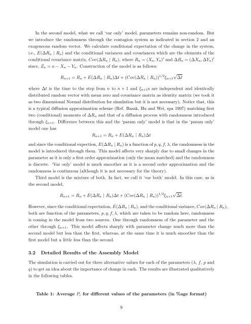
In the second model, what we call ‘var only’ model, parameters remains non-random. But
we introduce the randomness through the contagion system as indicated in section 2 and an
exogeneous random vector. We calculate conditional expectation of the change in the system,
i.e., E(∆R n | R n ) and the conditional variances and covariances which are the elements of the
conditional covariance matrix, Cov(∆R n | R n ), where R n = (X n , Y n ) ′ and ∆R n = (∆X n , ∆Y n ) ′
since, Z n = n − X n − Y n . Construction of the model is as follows:
√
R n+1 = R n + E(∆R n | R n )∆t + (Cov(∆R n | R n )) 1/2 ξ n+1 ∆t
where ∆t is the time to the step from n to n + 1 and ξ n+1 s are independent and identically
distributed random vector with mean zero and covariance matrix as identity matrix (we took it
as two dimensional Normal distribution for simulation but it is not necessary). Notice that, this
is a typical diffusion approximation scheme (Ref. Basak, Hu and Wei, spa 1997) matching first
two (conditional) moments of ∆R n and that of a diffusion process with randomness introduced
through ξ n+1 . Difference between this and the ‘param only’ model is that in the ‘param only’
model one has
R n+1 = R n + E(∆R n | R n )∆t
and since the conditional expection, E(∆R n | R n ) is a function of p, q, f, λ, the randomness in the
model is introduced through them. This model affects very sharply due to small changes in the
parameter as it is only a first order approximation (only the mean matched) and the randomness
is discrete. ‘Var only’ model is much smoother as it is a second order approximation and the
randomness is continuous (although it is not necessary for the theory).
Third model is the mixture of both. In fact, we call it ‘var both’ model. In this case, as in
the second model,
√
R n+1 = R n + E(∆R n | R n )∆t + (Cov(∆R n | R n )) 1/2 ξ n+1 ∆t.
However, since the conditional expectation, E(∆R n | R n ), and the conditional variance, Cov(∆R n | R n ),
both are function of the parameters, p, q, f, λ, which are taken to be random here, randomness
is coming in the model from two sources. One through randomness of the parameter and the
other through ξ n+1 . This model affects sharply with parameter change much more than the
second model but less than the first, whereas, at the same time it is much smoother than the
first model but a little less than the second.
3.2 Detailed Results of the Assembly Model
The simulation is carried out for three alternative values for each of the parameters (λ, f, p and
q) to get an idea about the importance of change in each. The results are illustrated qualitatively
in the following tables.
Table 1: Average P c for different values of the parameters (in %age format)
9