Stochastic Dynamic Models for Political Regime Change and ...

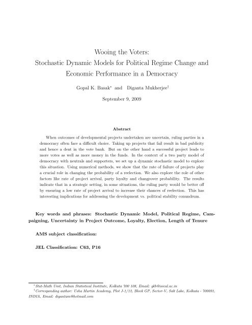
Wooing the Voters:
Stochastic Dynamic Models for Political Regime Change and
Economic Performance in a Democracy
Gopal K. Basak ∗ and Diganta Mukherjee †
September 9, 2009
Abstract
When outcomes of developmental projects undertaken are uncertain, ruling parties in a
democracy often face a difficult choice. Taking up projects that fail result in bad publicity
and hence a dent in the vote bank. But on the other hand a successful project leads to
more votes as well as more money in the funds. In the context of a two party model of
democracy with neutrals and supporters, we set up a dynamic stochastic model to explore
this situation. Using numerical methods, we show that the rate of failure of projects play
a crucial role in changing the probability of a reelection. We also explore the role of other
factors like rate of project arrival, party loyalty and changeover probability. The results
indicate that in a strategic setting, in some situations, the ruling party would be better off
by ensuring a low rate of project arrival to increase their chances of reelection. This has
interesting implications for addressing the development vs. political stability conundrum.
Key words and phrases:
Stochastic Dynamic Model, Political Regime, Campaigning,
Uncertainty in Project Outcome, Loyalty, Election, Length of Tenure
AMS subject classification:
JEL Classification: C63, P16
∗ Stat-Math Unit, Indian Statistical Institute, Kolkata 700 108, Email: gkb@isical.ac.in
† Corresponding author: Usha Martin Academy, Plot J-1/12, Block GP, Sector-V, Salt Lake, Kolkata - 700091,
INDIA, Email: digantam@hotmail.com

1 Introduction
In general, an improvement in political conditions will lead to faster and sustained growth. In
this scenario of politically enhanced growth, the effects of political institutions on growth may
persist over a long period of time (Barro 1997). For example, when a nation increases its
level of economic freedom from a minimal to a maximal level as the result of political change,
tremendous room will be created for long-run economic growth. The long-run growth rate of a
country is determined also by politics, along with economic behavior and demographic trends.
There is indeed a school of thought that political markets are inherently inefficient and
competition among the players causes excessive rent-seeking activity (Tullock 1967, 1983,
1989; McCormick et al. 1984). The existing literature, in the context of trade policy, also
argues that competitive rent-seeking results in an efficiency loss to the economy (Krueger 1974,
Bhagwati 1982, Grossman and Helpman 1994). Laband and Sophocleus (1992), for
instance, estimate that rent seeking in allocating transfers cost the US at least one-fourth of
its GDP in 1985. Also growth of government debt is positively related to the frequency of
government change De Haan and Strum 1994. Persson and Svensson (1989) have shown
that a conservative government, which favors a low level of government spending but knows that
it will probably be replaced by a government in favour of higher spending levels, will borrow
more than when it was certain to stay in office. In this context see also Alesina and Perotti
1996, Volkerink and De Haan 1999, Perotti and Kontopoulos 2002. Uppal (2009),
examines the effect of legislative turnover on government expenditures in a panel of 15 Indian
states during 1980-2000. He finds that political turnover promotes government expenditure (his
results are ribust with respect to alternative specifications of per capita or as percentage of
GDP). De Haan and Strum 1994 have examined whether the number of government changes
may help explain cross-country differences in public debt growth. It is very interesting that the
frequency of government changes apparently does matter. This result is broadly in accordance
with the conclusions of Grilli, Masciandaro and Tabellini, (1991). Jong-A-Pin and
De Haan (2007) finds that economic growth accelerations are preceded by economic reforms.
Furthermore, they find that growth accelerations are more likely to happen after the start of
a new political regime. The dataset used by them consists of 106 countries over the period
1957-1993 of which 57 countries experienced at least one growth acceleration. More specifically,
the findings are that the effect of economic reform on the probability of a growth acceleration is
highly significant in all specifications. However, the results for political regime changes are less
clear. Political regime changes are in general not related to growth accelerations, but there is a
negative and significant effect of regime duration for all specifications. This implies that growth
accelerations are more likely to happen after the start of a new political regime. For a survey
on the relationship between economic growth and political regimes see Przeworski, Alvarez,
Cheibub and Limongi (2000).
But there is also a counter literature, for instance in the development literature, that asserts
the concept of antagonistic growth, which refers to a situation where democratic governments
1

face the possibly untenable problem of resolving conflicting claims of vested interests while
concurrently pursuing sustainable paths for growth (Foxley, MacPherson and ODonnell
1986). Nordhaus (1975) shows that an opportunistic incumbent, who has an informational
advantage over the voters, follows a suboptimal policy right before elections to increase his or her
chances of reelection, leading to political business cycles. Besley and Burgess (2002) argue
that the resolution of informational disadvantage make the governments more accountable. They
find that state governments in India respond better to natural calamities where the newspaper
circulation, which mitigates the informational disadvantage of voters, is high.
Lyne (2008), in the context of democratic accountability and development in Brazil and
Venezuela, argues that the project choices made by the governments in these countries were
among the more economically inefficient alternatives available within an inward oriented program.
But policies that are economically inefficient can be highly politically advantageous in
a system where structural conditions favor the clientelistic equilibrium. If economically detrimental
policies maximize the transformation of government power and resources into goods for
quid pro quo exchange, then politicians competing in clientelistic systems will favor them over
economically superior choices. Despite the unfavorable economic consequences, permanent subsidies,
capital intensity and high and variable protection turn out to be the more competitive
political choice when voters opt for quid pro quo. Lahiri (2000) argues competitive politics in
India has damaged any chances of fiscal prudence by the states for the want of securing their
vote bank.
Feng (2005) has done a very interesting study of the interplay between economic performance
and political events with a simultaneous equations model with growth, government
change and degree of democracy as endogenous variables. Using data from several south-east
asian countries he shows that not only growth is stimulated by regime changes, in turn it also
facilitates regime changes. The results found are robust with respect to specifications.
Noting the interplay between the political process and the economic process, we try to model
the strategic role of elected policy makers in undertaking development projects whose outcomes
are uncertain. The activities considered for the ruling party are deciding to undertake and
executing development projects, whose outcomes are uncertain in nature. Thus the projects, if
undertaken, can be both beneficial or detrimental to the popularity of the ruling party. Also, the
budget available to the ruling party would be related to the decision of undertaking projects. A
successful project adds to the populatiry of the elected government but a failed one will reduce
their chances of being re-elected. Thus, the perceived or prevalent rate of success of development
projects could play a key role in the government’s decision to undertake such projects.
The process of a party coming to power in a democratic country depends on how the voters
support them in the elections. Although the election is a discrete event taking place at prespecified
intervals of time, the whole process of alluring/increasing voters/supporters to a party
(political campaigning process) goes on continuously between the elections. One usually also
holds the party accountable for its deeds when in power (public works, development projects
undertaken etc.) and votes accordingly. Or, at least that is the standard assumption.
2

Our aim is to study the voting process as a three population (X, Y, Z) model (for a two
party system with support base X and Y), with third population (Z) being passive towards any
party even though they cast votes during election (assumptions need be taken on their voting
behaviour also). We would like to study how, in an election X or Y becomes the winner and
how it depends on their deeds during the time interval between the two elections.
In this direction, understanding the dynamics of (X, Y, Z) under some suitable standard
assumptions would be important. Further, we would like to investigate what happens if the
standard assumptions are violated. We would develop relevant theoretical results and also simulate
the dynamics to see the changing pattern at different times and in the long run.
Specific theoretical questions:
1. What are the significant events for causing government change: Investment in campaigning
or new projects happening?
What would be the dynamics under the influence of such events.
2. What are the conditions conducive to continuance (one party staying in power over repeated
elections)? How to find P (x t+s > 1 2 |x t > 1 2 ) (x t being the share of X in the
population)?
3. What are the conditions for transition?
4. What would be reliable estimates of transition probabilities and what would be the form
of a long run distribution of the population in types X, Y and Z?
Section 2 describes our model with the alternative variations. The relevant theoretical discussions
on results, both for passive and strategic behaviour, are presented in several subsections.
The full Assembly model is discussed in section 3. In different subsections we discuss the modelling
strategy, empirical results and strategic considerations. Section 4 mentions a few possible
extensions to our basic model. These could be taken up in future work. Finally section 5
concludes.
2 The Two Party Model
2.1 Single Constituency (Local) Model
As mentioned above, the political parties engage in two kinds of activities. One of a developmental
nature where the ruling party execute projects. These projects arrive randomly at a rate
λ > 0 per unit of time. If taken up, it may result in a success or failure (with probability f).
A successful project results in additional funds for the ruling party as well as positive publicity.
Whereas a failed project creates negative publicity. Publicity (positive or negative) results in
increased or reduced support. In case of positive outcome, neutral or opposing party supporters
3

may join the ruling party (with some exogenously given probability p and (1 − p)). In case of
a failure the party supporters may leave the party and convert to neutral or opposing party
supporters with same probabilities (p and (1 − p)). The flow of events for this is depicted in the
figure below.
The second activity that both parties engage in is political campaigning with available funds
that helps in bringing opposition or neutrals to the party fold. The rate of conversion depends
on the fund spent and an exogenous loyalty parameter (q). Apart from these two party based
activities, there is also some switching over that happens autonomously through interaction
between the three types of individuals in the population. The rates of conversion are also exogenously
given.
[Please see Project tree diagram at the end]
First we start with passive players (non-strategic).
• Take time period ∆t = 1 month, so there will be 60 periods between elections.
First we study the probability of change at the first election, simulating 1000 times.
• Then we trace for 10 consecuive elections, 50 years (= 600 periods), simulating 1000 times.
To calculate average tenure / number of government changes in the 50 year period.
• Look at comparative statics, for alternative choices of parameter values.
{ }
X0 Y 0 Z 0
We start with a population distribution given by
40 35 25
We explore the dynamics for the following choice of values of the parameters:
λ : 0.1, 0.2, 0.3 rate of project arrival
f : 0.5, 0.7, 0.9 probability of failure
p : 0.2, 0.25, 0.3 probability of switching to Z due to project failure
q : 0.7, 0.8, 0.9 probability to stay on (not switch due to campaign)
Here q is the loyalty parameter ∈ (0, 1).
We may assume that either Z gets equally divided in time of voting or some random behaviour
(e.g. β fraction vote for Y where β ∼ B(λf + 1 2 , 1 2 ). So that E(β) = λf+ 1 2
λf+1 .)
Campaigning effects are modelled as follows:
For the ruling party, R n : γ 1 (R n )(1 − q) Yn
N
(for Y → X)
and γ 0 (R n ) Zn
N
(for Z → X)
and for the Opposition, O n :
γ 1 (x) = x
2+x
γ 0 (x) = x
1+x
and
γ 1 (O n )(1 − q) Xn
N
(for X → Y )
γ 0 (O n ) Zn
N
(for Z → Y )
4

R n (0) = 1 and R n (t + 1) = R n (t) + λ(1 − f).
O n = 1, constant over time.
The effect of interaction among the individuals in the population is given by the following
parameters depicting the tendency to switch:
Y → X β 1
X → Y β 1
Y → Z β −
X → Z β −
Z → Y β +
Z → X β +
The β parameters must be o( 1 N
) to keep the interaction effect in control. We choose the
following values:
β + = 0.3
β − = 0.2
β 1 = 0.1
With the above, the transition probabilities in the simplified 3-dimensional model can be
evaluated as follows (omitting time subscripts):
P (Y → X)
P (Z → X)
P (X → Z)
P (Y → Z)
P (X → Y )
P (Z → Y )
P (φ)
= γ 1 (R n )(1 − q) Y N + β 1 XY
N
= γ 0 (R n ) Z N + β + XZ
N
X(Y +Z)
= β − N
+ λfp X N
= β −
Y (X+Z)
N
= γ 1 (O n )(1 − q) X N + β 1 XY
N
= γ 0 (O n ) Z N + β + Y Z
N
= 1 - all of the above
+ λ(1 − f)(1 − p) Y N
+ λ(1 − f)p Z
N
+ λf(1 − p) X N
Hence, the change expectations are as follows:
E(∆X) = −(λf + γ 1 (O n )(1 − q)) X N + (γ 1(R n )(1 − q) + λ(1 − f)(1 − p)) Y N
+(γ 0 (R n ) + λ(1 − f)p) Z N − β XY
−
N
+ (β + − β − ) XZ
N
E(∆Y ) = (λf(1 − p) + γ 1 (O n )(1 − q)) X N − (γ 1(R n )(1 − q) + λ(1 − f)(1 − p)) Y N
+γ 0 (O n ) Z N − β XY
−
N
+ (β + − β − ) Y Z
N
E(∆Z) = λfp X N − (γ 0(R n ) + γ 0 (O n ) + λ(1 − f)p) Z N
XY
+2β −
N
− (β + − β − ) XZ
N
− (β + − β − ) Y Z
N
This is by construction closed, E(∆X) + E(∆Y ) + E(∆Z) = 0.
(1)
5

The second moments can be calculated as follows:
E(∆X) 2 = (λf + γ 1 (O n )(1 − q)) X N + (γ 1(R n )(1 − q) + λ(1 − f)(1 − p)) Y N
+(γ 0 (R n ) + λ(1 − f)p) Z N + (2β 1 + β − ) XY
N
+ (β + + β − ) XZ
N
E(∆Y ) 2 = (λf(1 − p) + γ 1 (O n )(1 − q)) X N + (γ 1(R n )(1 − q) + λ(1 − f)(1 − p)) Y N
+γ 0 (O n ) Z N + (2β 1 + β − ) XY
N
+ (β + + β − ) Y Z
N
E(∆Z) 2 = λfp X N + (γ 0(R n ) + γ 0 (O n ) + λ(1 − f)p) Z N + 2β −
+(β + + β − ) XZ
N
+ (β + + β − ) Y Z
N
XY
N
E(∆X∆Y ) = −(λf(1 − p) + γ 1 (O n )(1 − q)) X N + (γ 1(R n )(1 − q) + λ(1 − f)(1 − p)) Y N
−2β 1
XY
N
E(∆X∆Z) = −(γ 0 (R n ) + λ(1 − f)p) Z N − λfpX N − β −
E(∆Y ∆Z) = −γ 0 (O n ) Z N − β XY
−
N
− (β + + β − ) Y Z
N
XY
N
− (β + + β − ) XZ
N
(2)
2.2 Comparative Statics
We first study the probability of change P c at the end of one five year period (= 1 unit of time).
Consider the following expressions (this will hold if E(∆X) > 0 to start with, otherwise not
necessary):
1.
and
∂E(∆X)
∂f
∂E(∆Y )
∂f
= −λ X N − λ(1 − p) Y N − λp Z N < 0
= λ(1 − p) X N + λ(1 − p) Y N > 0
Also,
So, if X > Z then ∂E(∆X)2
∂f
∂E(∆X) 2
∂f
> 0. Therefore,
= λ X N − λ(1 − p) Y N − λp Z N
∂V (∆X)
∂f
> 0 if X > Z. Implies ∂Pc
∂f > 0.
6

2.
∂E(∆X)
∂λ
So f ≥ 1 2 ⇒ ∂E(∆X)
∂λ
< 0.
∂E(∆Y )
∂λ
Again, f ≥ 1 2 ⇒ ∂E(∆Y )
∂λ
> 0.
Also
Therefore,
∂V (∆X)
∂λ
∂E(∆X) 2
∂λ
= −f X N + (1 − f)(1 − p) Y N + (1 − f)p Z N
= f(1 − p) X N − (1 − f)(1 − p) Y N
= f X N + (1 − f)(1 − p) Y N + (1 − f)p Z N > 0
> 0 if f ≥ 1 2 . Implies, if f ≥ 1 2 , ∂Pc
∂λ > 0.
3.
So, Y < Z ⇒ ∂E(∆X)
∂p
> 0.
∂E(∆X)
∂p
= −λ(1 − f) Y N + λ(1 − f) Z N
∂E(∆Y )
∂p
= −λf X N + λ(1 − f) Y N
Therefore, f ≥ 1 2 ⇒ ∂E(∆Y )
∂p
4. No definitive answers for q
< 0. So, Y < Z, f ≥ 1 2 ⇒ ∂Pc
∂λ
< 0 likely.
We next simulate (∆X, ∆Y ) (in MATLAB) using N 2 (MVNRND command) with the above
moments (scaled by 1 month = dt = 1/60 = 0.0167) and generate ∆Z using the relation ∆Z =
−(∆X + ∆Y ). The main observations are as follows:
• If Z is bigger then P c decreases for f = 0.8. For f = 0.2, no pattern, for f = 0.5, there is
a mild decrease.
• For any distribution, ∂Pc
∂q > 0.
• ∂Pc
∂f > 0.
• For f = 0.5, ∂Pc
∂λ
increases in q.
• For any λ, ∂Pc
∂p
< 0 (for a fixed q).
We next study the (deterministic) pattern of change over time in the first moment of (X, Y, Z)
using a differential equation approach. To solve, we again use MATLAB (command: ODE45).
The results are qualitatively consistent with the stochastic approach.
7

2.3 Active Players
Finally, one needs to look at the Strategic Choice of λ in this. Here, the budget allocation may
be assumed to be identically distributed, and hence we may look at only one seat and solve the
allocation problem.
Recall that E(∆X) = −(λf + γ 1 (O n )(1 − q)) X N + (γ 1(R n )(1 − q) + λ(1 − f)(1 − p)) Y N
Therefore,
∂E
∂λ = −f X {
N + (1 − q)γ 1(R ′ n ) ∂R }
n
Y
∂λ + (1 − f)(1 − p)) N
= −f X N + { (1 − q)γ ′ 1(R n ) + (1 − p)) } (1 − f) Y N
(3)
if f is large (close to 1) then choice of λ would be close to 0.
3 Assembly Model
We now have multiple seats, shared between the two parties according to majority in each
constituency. Again we study the single elecion, tenure and comparative statics for
passive parties. To study the tenure pattern, we look at the pattern of government change over
a 50 year period with the stochastic approach.
In order to study the dynamics our proposed model in a robust way, we have carried out
simulation exercise with three variants of the model. One that considers the uncertainty in the
event probabilities only (model 1), the second considering the fluctuation through variance only
(model 2) and a final model (model 3) that considers both.
3.1 The Modelling Strategy
Here we have proposed three basic models each of which originated from a typical contagion
type model used in epidemiology. Contagion type of model of spread is used to come up with
the dynamic change of voter’s opinion that happens in a small time interval, say ∆t. We then
go on to use three type of modeling procedure to come up with the final models.
Basic idea is in a small time ∆t, when numbers of people in the three different group change,
(X n , Y n , Z n ) → (X n+1 , Y n+1 , Z n+1 ), since it is a small time interval and the total population has
been taken to be fixed (when growth of population is not considered), exactly one of the X, Y, Z
decreases causing exactly one of the other to increase. This event has been assumed to occur
with probability as in the contagion (disease) type model with some parameter p (probability of
switching to Z due to project failure), q (probability to stay on (not switch due to campaign)),
f (probability of failure) , λ (rate of project arrival) as mentioned in section 2.
Thus in the first model what we call ‘param only’ model we take these parameters to be
random and follow a Bernouli distribution (independent and different for different parameters)
indicating that the event occurs when Bernouli distribution takes the value 1, otherwise does
not occur. This model affects model very sharply with small changes in the parameter. We
compare this in the context of the other two models given below.
8

In the second model, what we call ‘var only’ model, parameters remains non-random. But
we introduce the randomness through the contagion system as indicated in section 2 and an
exogeneous random vector. We calculate conditional expectation of the change in the system,
i.e., E(∆R n | R n ) and the conditional variances and covariances which are the elements of the
conditional covariance matrix, Cov(∆R n | R n ), where R n = (X n , Y n ) ′ and ∆R n = (∆X n , ∆Y n ) ′
since, Z n = n − X n − Y n . Construction of the model is as follows:
√
R n+1 = R n + E(∆R n | R n )∆t + (Cov(∆R n | R n )) 1/2 ξ n+1 ∆t
where ∆t is the time to the step from n to n + 1 and ξ n+1 s are independent and identically
distributed random vector with mean zero and covariance matrix as identity matrix (we took it
as two dimensional Normal distribution for simulation but it is not necessary). Notice that, this
is a typical diffusion approximation scheme (Ref. Basak, Hu and Wei, spa 1997) matching first
two (conditional) moments of ∆R n and that of a diffusion process with randomness introduced
through ξ n+1 . Difference between this and the ‘param only’ model is that in the ‘param only’
model one has
R n+1 = R n + E(∆R n | R n )∆t
and since the conditional expection, E(∆R n | R n ) is a function of p, q, f, λ, the randomness in the
model is introduced through them. This model affects very sharply due to small changes in the
parameter as it is only a first order approximation (only the mean matched) and the randomness
is discrete. ‘Var only’ model is much smoother as it is a second order approximation and the
randomness is continuous (although it is not necessary for the theory).
Third model is the mixture of both. In fact, we call it ‘var both’ model. In this case, as in
the second model,
√
R n+1 = R n + E(∆R n | R n )∆t + (Cov(∆R n | R n )) 1/2 ξ n+1 ∆t.
However, since the conditional expectation, E(∆R n | R n ), and the conditional variance, Cov(∆R n | R n ),
both are function of the parameters, p, q, f, λ, which are taken to be random here, randomness
is coming in the model from two sources. One through randomness of the parameter and the
other through ξ n+1 . This model affects sharply with parameter change much more than the
second model but less than the first, whereas, at the same time it is much smoother than the
first model but a little less than the second.
3.2 Detailed Results of the Assembly Model
The simulation is carried out for three alternative values for each of the parameters (λ, f, p and
q) to get an idea about the importance of change in each. The results are illustrated qualitatively
in the following tables.
Table 1: Average P c for different values of the parameters (in %age format)
9

Model 1
p 0.2 0.25 0.3
avg. P c 31.33 31.15 30.52
q 0.7 0.8 0.9
avg. P c 28.07 31.81 33.11
λ 0.1 0.2 0.3
avg. P c 29.63 31.11 32.26
f 0.5 0.7 0.9
avg. P c 0 0 93
Model 2
p 0.2 0.25 0.3
avg. P c 24.74 22 22.22
q 0.7 0.8 0.9
avg. P c 21.33 23.07 24.56
λ 0.1 0.2 0.3
avg. P c 22.63 22.19 24.15
f 0.5 0.7 0.9
avg. P c 12.7 21.48 34.78
Model 3
p 0.2 0.25 0.3
avg. P c 20.26 21.56 19.81
q 0.7 0.8 0.9
avg. P c 18.41 20.11 23.11
λ 0.1 0.2 0.3
avg. P c 20.22 18.89 22.52
f 0.5 0.7 0.9
avg. P c 10.96 18.96 31.7
We first look at the change in average value of P c with one variable of the model at a time. In
all the three variants of the model P c changes very little with p or λ. There is also no monotonic
pattern. With changes in q, there does exist an increasing pattern but the rate of change is
small. The parameter that has the strongest effect on the value of P c is f which has a strong
positive effect in all three variants. So, unconditionally, f is seen to have the maximum effect
on rate of change. For model 1, it suddenly jumps to 93% from 0 when value of f becomes 0.9.
In the other cases also the probability of change is around 10% when f is 0.5 and becomes more
than 30% for f = 0.9.
Table 2: Conditional effect of the parameters on P c
Results are presented in the order of the models (1,2,3)
10

λ f p q
P c |f (+,+,+)
P c |q (+,0,+)
P c |λ (0,+,0)
P c |q (0,+,+)
P c |λ (+,0,0)
P c |f (+,+,+)
P c |q (0,0,+)
P c |f (+,+,+)
P c |λ (+,0,0)
The corresponding detailed results are presented in the three dimensional plots in figures at
the end of the paper.
As there might be cross effects in conjunction with other parameters, we investigate this by
fixing the other parameters at each level and study the effect of each parameter on P c . Conditioal
on other parameters, the failure rate, f, has the maximum impact in the expected direction on
the probability of change. With a rising f, P c also rises. We find that if we fix f or q (loyalty)
then conditionally λ has the expected positive effect also.
Coming to the switching parameter p, again conditional results are quite definitive, P c rises
in p for fixed level of λ, f or q. Finally, the loyalty parameter q has the same effect for any level
of f and λ. Other conditioning values turn out to be non-monotonic.
As a conditioning factor, f has the maximum impact on the results as all the parameters
λ, p and q raises P c in all the three variants of the model for each fixed level of f. The second
most important conditioning factor is q. The effect of λ, f and q on P c , conditionally on p, is
non-monotonic. This implies that switch parameter plays the role of a strategy shifter. The
optimal behaviour of the political parties in terms of controlling the value of λ (project arrival
rate) will be different for different levels of p.
Looking at the distribution of the length of tenure (see figure at the end of the paper) in
all three variants of the model, it can be easily seen that the average length increases as we
introduce more variation in the model (from model 1 to 2 to 3). This corroborates the finding
in Table 1 that the rate of change is higher in model 1 than in model 2 and 3.
3.3 Strategic Players
We now move on to the strategic part, but now the choice of both λ as well as campaign
budget allocation among different seats needs to be studied.
So the objective would be to MaxE(∆X) etc. over λ and over simultaneous choice of
{R ni , O ni }, i = seats and n = time.
11

We know that ∑ seats R ni = R n = R n−1 + λ(1 − f), so it depends on λ again. ∑ seats O ni =
O n = 1.
So a stochastic optimal control problem to be formulated.
For budget allocation we have,
∂E
∂R ni
= γ ′ 1 (R ni)(1 − q) Y i
N i
Therefore, the marginal condition will imply γ 1 ′ (R ni)(1 − q) Y i
N i
Thus, y i > y j
concave.
Then, for choice of λ,
= γ ′ 1 (R ni)(1 − q)y i (say).
= γ 1 ′ (R nj)(1 − q) Y j
N j
= τ (say).
⇒ γ 1 ′ (R ni) < γ 1 ′ (R nj) ⇒ R ni > R nj , as γ 1 is assumed to be increasing and
∑
i
∂E(X i )
∂λ
= ∑ i
[ −fXi + (1 − f)y i
{ (1 − q)γ
′
i (R ni ) + (1 − p) }]
= −f ∑ i
x i + (1 − f)(1 − q) ∑ i
y i γ ′ 1(R ni ) + (1 − f)(1 − p) ∑ i
y i
= −f ∑ i
x i + (1 − f)(1 − p) ∑ i
y i + (1 − f)Kτ
= K [f ¯x + (1 − f)(1 − p)ȳ + (1 − f)τ] (4)
If X is small in a particular seat and τ is large (i.e. q small, less loyalty), then ruling party
may choose a large λ.
3.4 Empirical Issues
1. As we have assumed dt = 0.0167 = 1 month in calendar time, then one needs to carefully
calibrate the population size also (1 lac or 1 million preferred) so that we can have λ =
0.1 / 0.2 / 0.3 realistically.
2. We would like to estimate the relevant parameters of the model for a given democracy and
make estimates and forecasts (calibration exercise). So to estimate λ and f from actual
data (MOU vs. project actually happening)
3. Also, comparing the estimates and forecasts for two democratic systems would be an
interesting issue.
4 Possible Extensions
• We propose to generalize the model to accomodate a multi-party system.
• We started with the 3-dimensional model (X, Y, Z). One then needs to go on to the 5-
dimensional model (X m , X s , Z, Y s , Y m ), distinguishing between members and supporters.
• Possible asymmetry in campaigning: We can consider that the campaigning effects
are asymmetric across consituencies. Then the budget allocation may also be asymmetric.
To study the optimisation problem in this situation.
12

• Asymmetric perception of failure rate: Information does not reach all equally well.
If perceived ”fail” is low for some people, does it help longer tenures?
Suggested solution: introduce a stochastic ”f”. Higher variance (more information asymmetry,
feature of LDCs) ⇒ longer tenure?
• Population growth: If all groups grow equally, then no change in proportions and results
unchanged.
If Z grows faster than X or Y, then may assume Z has net growth, X & Y stationary. Also
the reverse case. Results to be studied.
X, Y grows at rate α 1 and Z grow at rate α 2 . Then cases to be considered are
(i) α 1 = α 2
(ii) α 1 > α 2
(iii) α 1 < α 2 .
• Episodic event: War or Natural Calamity. Should have both short term and long term
impact. May be modelled by ”delay” equations.
5 Concluding Remarks
When outcomes of developmental projects undertaken are uncertain, ruling parties in a democracy
often face a difficult choice. Taking up projects that fail result in bad publicity and hence
a dent in the vote bank. But on the other hand a successful project leads to more votes as well
as more money in the funds. In the context of a two party model of democracy with neutrals
and supporters, we set up a dynamic stochastic model to explore this situation.
Using numerical methods, we show that the rate of failure of projects play a crucial role in
changing the probability of a reelection. We also explore the role of other factors like rate of
project arrival, party loyalty and changeover probability. We have studied the unconditional and
conditional (fixing the value of other parameters at different levels) effect of all the parameters
on the probability of change. The results throw up some interesting patterns on joint effects
that are quite intriguing and calls for further research.
The results indicate that in a strategic setting, in some situations, the ruling party would be
better off by ensuring a low rate of project arrival to increase their chances of reelection. This
has interesting implications for addressing the development vs. political stability conundrum.
The model that we have considered here relies on three alternative formulations of the
uncertainty inherent in the situation under study. The results are accordingly more or less
sensitive to changes in the value of the parameters. A comparative study of this has also been
made.
In the sequel we have pointed out some possible future directions of research in this area.
there are many interesting alternatives to be explored both theoretically or numerically as well
as empirically using available databases or primary data specifically collected for this purpose.
13

References
1. Alesina, A. and R. Perrotti (1996). Income distribution, political instability, and investment.,
European Economic Review, 40, 1203-28.
2. Robert J. Barro, 1997. Myopia and Inconsistency in the Neoclassical Growth Model,
NBER Working Papers 6317, National Bureau of Economic Research, Inc.
3. Besley, T. and R. Burgess (2002). The political economy of government responsiveness:
theory and evidence from India, Quarterly Journal of Economics, 4, 1415-51.
4. Bhagwati, J. (1982). Directly Unproductive Profit-Seeking (DUP) Activities, Journal of
Political Economy, 90(5), 988-1002.
5. De Haan, J., and J. Strum (1994). Political and institutional determinants of fiscal policy
in the European Community, Public Choice, 80, 157-72.
6. Feng, Y. (2005). Democracy, Governance, and Economic Performance: Theory and Evidence,
MIT Press.
7. Foxley, Alejandro, Michael S. MacPherson and Guillermo ODonnell (1986). Development,
Democracy, and the Art of Trespassing: Essays in Honor of Albert O. Hirschman (Notre
Dame: The University of Notre Dame Press).
8. Grilli, V., Masciandaro, D. and Tabellini, G. (1991). Political and monetary institutions
and pub- lic financial policies in the industrial countries. Economic Policy, Nr. 13: 341-392.
9. Grossman, G. and E. Helpman (1994). Protection for Sale, American Economic Review,
84(4), 833-50.
10. Jong-A-Pin, R. and J. De Haan (2007). Political Regime Change, Economic Reform And
Growth Accelerations, Cesifo Working Paper No. 1905.
11. Krueger, A. (1974). The political economy of the rent-seeking society, American Economic
Review, 64(3), 291-303.
12. Laband, D. and John P. Sophocleus (1992). An estimate of resource expenditures of
transfer activity in the United States, Quarterly Journal of Economics, 107(3), 959-83.
13. Lahiri, A. (2000). Sub-national public finance in India, Economic and Political Weekly,
35(18), 1539-49.
14. Lyne, M. M. (2008). The Voters Dilemma and Democratic Accountability: Explaining
the Democracy-Development Paradox, forthcoming, The Pennsylvannia State University
Press.
14

15. McCormick, R. E.,W. F. Shughart II, and R. E. Tollison (1984). The disinterest in deregulation,
American Economic Review, 74(5), 1075-79.
16. Nordhaus, W. D. (1975). The political business cycle, Review of Economic Studies, 42(2),
169-90.
17. Perotti, R., and Y. Kontopoulos (2002). Fragmented fiscal policy, Journal of Public Economics,
86, 191-222.
18. Persson, T., and L. E. O. Svensson (1989). Why a stubborn conservative would run a
deficit policy with time-inconsistent preferences, Quarterly Journal of Economics, 104(2),
325-45.
19. Przeworski, A., Alvarez, M., Cheibub, J. A. and Limongi, F. (2000), Democracy and
Development: Political Regimes and Economic Well-being in the World, 1950-1990, New
York: Cambridge University Press.
20. Tullock, G. (1967). The welfare costs of tariffs, monopolies and thefts, Western Economic
Journal, 5, 224-32.
21. Tullock, G. (1983). Economics of income redistribution. Boston, MA: Kluwer-Nijhoff.
22. Tullock, G. (1989). The economics of special privilege and rent seeking. Boston,MA:
Kluwer-Nijhoff.
23. Uppal, Y. (2009). Does legislative turnover adversely affect state expenditure policy?
Evidence from Indian state elections, mimeo, Department of Economics, Youngstown State
University, USA.
24. Volkerink, J., and J. De Haan (2001). Fragmented government effects on fiscal policy:
New evidence, Public Choice, 109, 221-42.
15

Project Tree Diagram
(1-p)
X → Y: λ f (1-p) X n
Failure (f) X → Z: λf p X n
p
Project (rate
of arrival λ)
Success (1-f) (1-p) Y → X: λ (1- f) (1-p) Y n
P
Z → X: λ (1- f) p Z n
16

Model 1
count change
100
50
1 0
0.8
0.6
f
0
0.2
lamda
0.4
count change
35
30
0.4
25
0.3
p
0.2
0
0.2
lamda
0.4
count change
35
30
25
0.9 0.8
0.7
q
0
0.2
lamda
0.4
count change
100
50
0.4 0
0.3
p
0.2
0.6
f
0.8
1
count change
100
50
18
0
0.9 0.8
0.7
q
0.6
f
0.8
1
count change
35
30
25
0.9 0.8
0.7
q
0.2
p
0.3
0.4

Model 2
count change
40
20
0
1
0.8
0.6
f
0
0.2
lamda
0.4
count change
30
25
0.4
20
0.3
p
0.2
0
0.2
lamda
0.4
count change
30
25
20
0.9 0.8
0.7
q
0
0.2
lamda
0.4
count change
40
20
0.4 0
0.3
p
0.2
0.6
f
0.8
1
count change
40
20
19
0
0.9 0.8
0.7
q
0.6
f
0.8
1
count change
30
20
10
0.9 0.8
0.7
q
0.2
p
0.3
0.4

Model 3
count change
40
20
0
1
0.8
0.6
f
0
0.2
lamda
0.4
count change
25
20
0.4
15
0.3
p
0.2
0
0.2
lamda
0.4
count change
30
20
10
0.9 0.8
0.7
q
0
0.2
lamda
0.4
count change
40
20
0.4 0
0.3
p
0.2
0.6
f
0.8
1
count change
40
20
20
0
0.9 0.8
0.7
q
0.6
f
0.8
1
count change
25
20
15
0.9 0.8
0.7
q
0.2
p
0.3
0.4

Model 1
Model 2
Model 3
21