Numerical Solution of Cauchy Problems for Elliptic ... - COMSOL.com
Numerical Solution of Cauchy Problems for Elliptic ... - COMSOL.com
Numerical Solution of Cauchy Problems for Elliptic ... - COMSOL.com

You also want an ePaper? Increase the reach of your titles
YUMPU automatically turns print PDFs into web optimized ePapers that Google loves.
Presented at the <strong>COMSOL</strong> Multiphysics User's Conference 2005 Boston<br />
<strong>Numerical</strong> <strong>Solution</strong> <strong>of</strong> <strong>Cauchy</strong> <strong>Problems</strong> <strong>for</strong><br />
<strong>Elliptic</strong> Equations in “Rectangle-like”<br />
Geometries<br />
Fredrik Berntsson and Lars Eldén<br />
Department <strong>of</strong> Mathematics, Linköping University<br />
Oktober 2005<br />
– Femlab Conference 2005 –
Presented at the <strong>COMSOL</strong> Multiphysics User's Conference 2005 Boston<br />
Overview<br />
• Introduction, Motivating Example<br />
• Ill–posedness, Stabilization<br />
• <strong>Numerical</strong> Test problem in FEMLAB<br />
• Trans<strong>for</strong>mation to rectangular geometry. Mapping <strong>of</strong> Normal derivatives.<br />
• <strong>Numerical</strong> solution <strong>of</strong> Test problem<br />
• Conclusions, Future Work<br />
– Femlab Conference 2005 – 1
Presented at the <strong>COMSOL</strong> Multiphysics User's Conference 2005 Boston<br />
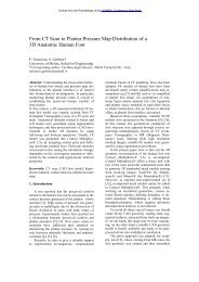
Motivating example: Ilmenite iron melting furnace<br />
Thermocouple<br />
Electrode<br />
Level K to<br />
level D<br />
thermocouples<br />
with level K<br />
highest<br />
Center<br />
Under<br />
electrodes<br />
Between<br />
electrodes<br />
The furnace material properties are temperature dependent.<br />
Problem: find the inner shape <strong>of</strong> the furnace.<br />
Nonlinear, and (rather) <strong>com</strong>plex geometry<br />
PhD thesis: I M Skaar, Monitoring the Lining <strong>of</strong> a Melting Furnace, NTNU, Trondheim, 2001<br />
– Femlab Conference 2005 – 2
Presented at the <strong>COMSOL</strong> Multiphysics User's Conference 2005 Boston<br />
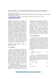
Irregular geometry - non-constant coefficient<br />
Map the region to a rectangle:<br />
liquid steel<br />
liquid steel<br />
<strong>Cauchy</strong> data<br />
Find lining: the interface between iron and furnace<br />
– Femlab Conference 2005 – 3
Presented at the <strong>COMSOL</strong> Multiphysics User's Conference 2005 Boston<br />
The <strong>Cauchy</strong> Problem <strong>for</strong> Laplace’s equation<br />
Classical ill-posed problem (Hadamard, 1900-1930)<br />
u xx + u yy = 0,<br />
u(x,0) = 0, −∞ ≤ x ≤ ∞,<br />
∂u<br />
∂x (x, 0) = 1 sin(nx), −∞ ≤ x ≤ ∞.<br />
n<br />
<strong>Solution</strong>:<br />
u(x,y) = 1 sin(nx) sinh(ny).<br />
n2 Large n: arbitrarily small data, arbitrarily large solution.<br />
The solution does not depend continuously on the data!<br />
– Femlab Conference 2005 – 4
Presented at the <strong>COMSOL</strong> Multiphysics User's Conference 2005 Boston<br />
Ill–posed <strong>Cauchy</strong> Problem on Unit Square<br />
y<br />
1<br />
(a(u)u x ) x +(a(u)u y ) y<br />
u x =0 u x =0<br />
u=g, u y =h<br />
1 x<br />
– Femlab Conference 2005 – 5
Presented at the <strong>COMSOL</strong> Multiphysics User's Conference 2005 Boston<br />
By separation <strong>of</strong> variables:<br />
Fourier analysis<br />
T(x,y)=A 0 y + B 0 +<br />
∞∑<br />
(A k e kπy + B k e −kπy )cos(kπx),<br />
k=1<br />
Fourier coefficients {A k } and {B k } satisfy (<strong>for</strong> k>0):<br />
( ) ( ) ( )<br />
1 1 Ak ĝk<br />
= ,<br />
kπ −kπ B k ĥ k<br />
where {ĝ k } and {ĥk} are the Fourier–cosine coefficients <strong>of</strong> g(x) and h(x)<br />
Since e kπy → ∞ as k → ∞ the problem is severely ill–posed!<br />
– Femlab Conference 2005 – 6
Presented at the <strong>COMSOL</strong> Multiphysics User's Conference 2005 Boston<br />
Rewrite as an Initial value problem:<br />
( ) (<br />
u 0 a<br />
=<br />
−1<br />
au y<br />
y<br />
− ∂<br />
∂x a ∂<br />
∂x<br />
0<br />
) (<br />
u<br />
au y<br />
)<br />
, 0≤y ≤1,<br />
(<br />
u(x, 0)<br />
u y (x, 0)<br />
) ( )<br />
g<br />
= .<br />
h<br />
The unbounded x-derivative makes the problem ill-posed!<br />
Approximation <strong>of</strong> derivative:<br />
∂<br />
∂x<br />
(<br />
a(u) ∂v )<br />
∂x<br />
≈ ¯D(A ¯DV )<br />
A diagonal matrix, depends on u<br />
¯D bounded differentiation matrix, spectral or otherwise<br />
Resulting stable problem is solved using standard code (ode45) in Matlab.<br />
– Femlab Conference 2005 – 7
Presented at the <strong>COMSOL</strong> Multiphysics User's Conference 2005 Boston<br />
Approximate u(x) by a least squares cubic spline s(x).<br />
Then set u ′ (x)≈s ′ (x).<br />
α −3<br />
α −2<br />
α −1<br />
α 0<br />
α 1<br />
α 2<br />
α 3<br />
α 4<br />
α 5<br />
α 6<br />
α 7<br />
The basis functions Bj 3 (x), <strong>for</strong> j =−1,...,5.<br />
Choose a coarse grid =⇒ bounded differentiation operator.<br />
Advantage: flexible at boundaries.<br />
– Femlab Conference 2005 – 8
Presented at the <strong>COMSOL</strong> Multiphysics User's Conference 2005 Boston<br />
A <strong>Numerical</strong> Model Problem<br />
The Heat Equation<br />
(a(u)u x ) x + (a(u)u y ) y =0, in Ω<br />
Boundary Conditions<br />
∂u<br />
u = g,<br />
∂n = h, on L 1,<br />
∂u<br />
∂n = 0, on L 2 and L 3 ,<br />
– Femlab Conference 2005 – 9
Presented at the <strong>COMSOL</strong> Multiphysics User's Conference 2005 Boston<br />
Test problem generated in FEMLAB<br />
Sides: insulated<br />
Upper boundary: 1450 o<br />
Lower boundary: 800 o<br />
Temperature-dependent<br />
conductivity<br />
– Femlab Conference 2005 – 10
Presented at the <strong>COMSOL</strong> Multiphysics User's Conference 2005 Boston<br />
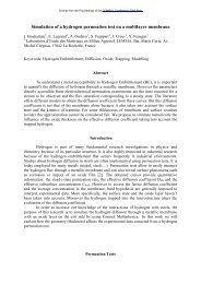
18<br />
Thermal conductivity<br />
16<br />
Thermal conductivity [ W/m o C ]<br />
14<br />
12<br />
10<br />
8<br />
6<br />
4<br />
2<br />
0 200 400 600 800 1000 1200 1400 1600<br />
Temperature [ o C ]<br />
The thermal conductivity <strong>for</strong> magnesia brick, as a function <strong>of</strong> temperature.<br />
– Femlab Conference 2005 – 11
Presented at the <strong>COMSOL</strong> Multiphysics User's Conference 2005 Boston<br />
Constructed solution (direct problem solved using FEMLAB):<br />
Temperature and Heat-Flux data along the lower boundary is used to<br />
identify the upper boundary!<br />
– Femlab Conference 2005 – 12
Presented at the <strong>COMSOL</strong> Multiphysics User's Conference 2005 Boston<br />
Trans<strong>for</strong>mation <strong>of</strong> the Problem<br />
The Con<strong>for</strong>mal Mapping<br />
(x, y) = φ(ξ,η) = [x(ξ, η), y(ξ, η)]<br />
The problem is trans<strong>for</strong>med into<br />
⎧<br />
⎪⎨<br />
⎪⎩<br />
(a(v)v ξ ) ξ + (a(v)v η ) η = 0, 0
Presented at the <strong>COMSOL</strong> Multiphysics User's Conference 2005 Boston<br />
Trans<strong>for</strong>mation <strong>of</strong> the area<br />
3.5<br />
3<br />
2.5<br />
2<br />
1.5<br />
1<br />
0.5<br />
0<br />
−0.5<br />
−1<br />
−1.5<br />
−2<br />
−3 −2 −1 0 1 2 3<br />
Con<strong>for</strong>mal mapping <strong>of</strong> the auxilliary domain onto a rectangle. Actual grid<br />
is finer!<br />
– Femlab Conference 2005 – 14
Presented at the <strong>COMSOL</strong> Multiphysics User's Conference 2005 Boston<br />
Computed flux data on the square<br />
4600<br />
4400<br />
4200<br />
4000<br />
3800<br />
3600<br />
3400<br />
3200<br />
−2 −1.5 −1 −0.5 0 0.5 1 1.5 2<br />
Trans<strong>for</strong>med using Con<strong>for</strong>mal mapping (blue curve). No noise added!<br />
– Femlab Conference 2005 – 15
Presented at the <strong>COMSOL</strong> Multiphysics User's Conference 2005 Boston<br />
Computed heat-flux on original Domain<br />
3500<br />
3000<br />
2500<br />
2000<br />
1500<br />
1000<br />
500<br />
0 1 2 3 4 5 6<br />
The Heat-Flux ∂u<br />
∂n on L 1 <strong>com</strong>puted by FEMLAB<br />
– Femlab Conference 2005 – 16
Presented at the <strong>COMSOL</strong> Multiphysics User's Conference 2005 Boston<br />
Trans<strong>for</strong>mation <strong>of</strong> normal derivatives<br />
By the Con<strong>for</strong>mal mapping<br />
∂u<br />
∂n | L1=|(φ −1 ) ′ | ∂v (ξ, 0)<br />
∂η<br />
The Schwarz–Christ<strong>of</strong>fel mapping function φ has a singularity at every<br />
corner <strong>of</strong> the polygonal domain.<br />
The Singularities in |(φ −1 ) ′ | almost cancel out the spikes in FEMLABs<br />
normal derivative.<br />
– Femlab Conference 2005 – 17
Presented at the <strong>COMSOL</strong> Multiphysics User's Conference 2005 Boston<br />
<strong>Numerical</strong> <strong>Solution</strong> <strong>of</strong> the Test problem<br />
liquid steel<br />
liquid steel<br />
<strong>Cauchy</strong> data<br />
• Solve <strong>Cauchy</strong> problem. Find the isotherm v=1450 o C.<br />
• Con<strong>for</strong>mal mapping <strong>of</strong> the identified curve.<br />
– Femlab Conference 2005 – 18
Presented at the <strong>COMSOL</strong> Multiphysics User's Conference 2005 Boston<br />
4500<br />
Noisy flux data<br />
4000<br />
3500<br />
3000<br />
−2 −1.5 −1 −0.5 0 0.5 1 1.5 2<br />
Normally distributed noise added. Realistic noise level!<br />
– Femlab Conference 2005 – 19
Presented at the <strong>COMSOL</strong> Multiphysics User's Conference 2005 Boston<br />
Computed temperatures at 0.6 and 0.8<br />
1340<br />
<strong>Numerical</strong> solution at y=0.60<br />
1460<br />
<strong>Numerical</strong> solution at y=0.80<br />
1320<br />
1440<br />
1300<br />
1420<br />
1280<br />
1400<br />
Temperature [ o C ]<br />
1260<br />
1240<br />
1220<br />
Temperature [ o C ]<br />
1380<br />
1360<br />
1340<br />
1200<br />
1320<br />
1180<br />
1300<br />
1160<br />
1280<br />
1140<br />
0 0.1 0.2 0.3 0.4 0.5 0.6 0.7 0.8 0.9 1<br />
1260<br />
0 0.1 0.2 0.3 0.4 0.5 0.6 0.7 0.8 0.9 1<br />
Derivatives <strong>com</strong>puted using 11 B-splines. Differential equation only valid<br />
when temperature is below 1450 o C.<br />
– Femlab Conference 2005 – 20
Presented at the <strong>COMSOL</strong> Multiphysics User's Conference 2005 Boston<br />
Noisy data, identified boundary<br />
4<br />
3<br />
2<br />
1<br />
0<br />
−1<br />
−2<br />
−3 −2 −1 0 1 2 3<br />
Derivatives <strong>com</strong>puted using 11 B-splines.<br />
– Femlab Conference 2005 – 21
Presented at the <strong>COMSOL</strong> Multiphysics User's Conference 2005 Boston<br />
Less regularization, temperature at 0.62 and 0.81<br />
1400<br />
<strong>Numerical</strong> solution at y=0.62<br />
1460<br />
<strong>Numerical</strong> solution at y=0.81<br />
1440<br />
1350<br />
1420<br />
1400<br />
Temperature [ o C ]<br />
1300<br />
1250<br />
Temperature [ o C ]<br />
1380<br />
1360<br />
1340<br />
1320<br />
1200<br />
1300<br />
1280<br />
1150<br />
0 0.1 0.2 0.3 0.4 0.5 0.6 0.7 0.8 0.9 1<br />
1260<br />
0 0.1 0.2 0.3 0.4 0.5 0.6 0.7 0.8 0.9 1<br />
Derivatives <strong>com</strong>puted using 19 B-splines!<br />
Impossible to identify boundary when the temperature is not smooth<br />
– Femlab Conference 2005 – 22
Presented at the <strong>COMSOL</strong> Multiphysics User's Conference 2005 Boston<br />
Conclusions<br />
• Efficient solution: replace a derivative by bounded approximation, solve<br />
<strong>Cauchy</strong> problem stably using a “method <strong>of</strong> lines”<br />
• General geometries: trans<strong>for</strong>m “rectangle-like region” to rectangle<br />
(equivalent to creating a curvilinear mesh). Solve the problem on<br />
the rectangle<br />
• Trans<strong>for</strong>mation cheap to <strong>com</strong>pute <strong>for</strong> rather general geometries<br />
(approximated by polygon)<br />
• Nonlinear problems can be solved rather easily<br />
• Stability theory: A stability estimate <strong>for</strong> a <strong>Cauchy</strong> problem <strong>for</strong> an elliptic<br />
partial differential equation, Inverse <strong>Problems</strong>, vol. 21, no 5, pp. 1643-<br />
1653, October 2005.<br />
– Femlab Conference 2005 – 23
Presented at the <strong>COMSOL</strong> Multiphysics User's Conference 2005 Boston<br />
Future Work<br />
• More detailed FEMLAB model <strong>of</strong> the Furnace. More realistic simulation<br />
<strong>of</strong> measurements.<br />
• Identify boundaries given other conditions (e.g. insulated boundary).<br />
• Applications: The Melting Furnace<br />
• Use FEMLAB to creat Test problem. Finding good test problems is very<br />
important!<br />
– Femlab Conference 2005 – 24

![[PDF] Comsol conference proceedings ... - COMSOL.com](https://img.yumpu.com/50379146/1/190x245/pdf-comsol-conference-proceedings-comsolcom.jpg?quality=85)