
Create successful ePaper yourself
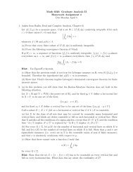
Turn your PDF publications into a flip-book with our unique Google optimized e-Paper software.
<strong>TikZ</strong> /<strong>PGF</strong> <strong>and</strong> <strong>other</strong> L A TEX <strong>Tricks</strong><br />
Erica Shannon<br />
Contents<br />
1 Resources 1<br />
2 Polygons 2<br />
3 Subgroup Lattices 3<br />
4 Coxeter graphs <strong>and</strong> Dynkin diagrams 4<br />
5 Tableau(x) 5<br />
6 Graphs of Functions 6<br />
7 Vector Diagrams / Root Systems 11<br />
8 Adding extra space in tables 14<br />
<strong>TikZ</strong> st<strong>and</strong>s for <strong>TikZ</strong> ist kein Zeichenprogramm; <strong>PGF</strong> st<strong>and</strong>s for Portable Graphics Format.<br />
1 Resources<br />
• Comprehensive <strong>TikZ</strong> Manual:<br />
http://ftp.math.purdue.edu/mirrors/ctan.org/graphics/pgf/base/doc/generic/pgf/pgfmanual.<br />
pdf<br />
• pgfplots Manual:<br />
http://www.bakoma-tex.com/doc/latex/pgfplots/pgfplots.pdf<br />
• A nice tutorial for basic drawing using <strong>TikZ</strong> :<br />
http://www.math.uni-leipzig.de/~hellmund/LaTeX/pgf-tut.pdf<br />
• List of colors available from the dvipsnames package:<br />
http://en.wikibooks.org/wiki/LaTeX/Colors<br />
1
2 Polygons<br />
Here are some triangles with labels.<br />
1<br />
2<br />
π/3<br />
1<br />
√<br />
2<br />
2<br />
π/4<br />
1<br />
π/6<br />
π/4<br />
√<br />
3<br />
√<br />
2<br />
2<br />
2<br />
Here are some regular polygons, drawn using the foreach comm<strong>and</strong> for loops.<br />
n = 3 n = 4 n = 5<br />
n = 6 n = 7 n = 8<br />
The <strong>TikZ</strong> manual has examples of how to draw pretty much any type of shape or diagram<br />
you might come up with. In particular, there’s a list of cool available node shapes starting<br />
on p.435. (Forbidden sign, clouds, magnifying glass, starburst, etc.)<br />
2
3 Subgroup Lattices<br />
There is supposed to be a <strong>TikZ</strong> library (graphs) for typesetting graphs. However, I found it<br />
extremely difficult to get this library to work correctly (or at all!). As a result, the examples<br />
here are made using the st<strong>and</strong>ard <strong>TikZ</strong> nodes <strong>and</strong> lines.<br />
S 3<br />
〈(123)〉<br />
〈(13)〉<br />
〈(23)〉<br />
〈(13)〉<br />
{e}<br />
Here’s a more complicated one:<br />
D 8 = 〈r, s〉<br />
〈s, r 2 〉 〈r〉<br />
〈sr, r 2 〉<br />
〈sr 2 〉 〈s〉 〈r 2 〉 〈sr 3 〉 〈sr〉<br />
{e}<br />
3
4 Coxeter graphs <strong>and</strong> Dynkin diagrams<br />
Finite Coxeter groups can be classified by their Coxeter graphs.<br />
A n<br />
E 7<br />
· · ·<br />
B n<br />
4<br />
· · ·<br />
E 6 I 2 (m)<br />
m<br />
C n · · ·<br />
4<br />
E 8<br />
F 4<br />
4<br />
D n<br />
· · ·<br />
H 3<br />
5<br />
H 4<br />
5<br />
If Φ is an irreducible root system of rank l, its Dynkin diagram is one of the following (l<br />
vertices in each case):<br />
A l<br />
E 6<br />
· · ·<br />
D l · · ·<br />
B l · · ·<br />
E 7<br />
C l · · ·<br />
E 8<br />
F 4<br />
G 2<br />
4
5 Tableau(x)<br />
Here’s a st<strong>and</strong>ard Young tableau.<br />
1 4 5 10 11<br />
2 6 8<br />
3 9 12<br />
7<br />
Here’s a domino tableau.<br />
1<br />
4<br />
3<br />
6<br />
5<br />
2<br />
Both of these images use macros from Tyson Gern – you’ll need to copy these from the<br />
header section.<br />
5
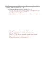
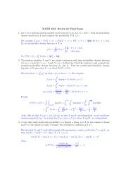
6 Graphs of Functions<br />
Here’s a simple graph of the function f(x) = x − x2<br />
2 + 1.<br />
3<br />
2<br />
1<br />
−2 −1 1 2<br />
−1<br />
−2<br />
−3<br />
Here’s a graph of a piecewise linear function, with background grid.<br />
2<br />
1<br />
−2 −1 1 2 3<br />
−1<br />
−2<br />
−3<br />
6
Here’s a graph of f(x) = sin(x) − cos(x), with a shaded region.<br />
1<br />
y<br />
f(x) = sin(x) − cos(x)<br />
x<br />
π<br />
4<br />
π<br />
2<br />
3π<br />
4<br />
π<br />
5π<br />
4<br />
3π<br />
2<br />
−1<br />
Here’s an<strong>other</strong> graph, this time with an annoyingly starred region. See p.393 of the <strong>TikZ</strong><br />
manual for a list of patterns.<br />
10<br />
y<br />
8<br />
6<br />
f(x) = 6 − 4 sin(x)<br />
4<br />
2<br />
1 2 3 4<br />
x<br />
Here’s a function <strong>and</strong> its tangent line. This graph has a legend.<br />
1<br />
ln(2)<br />
y<br />
1 2<br />
x<br />
f(x) = ln(x)<br />
y = x − 1<br />
7
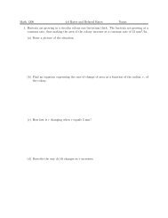
Here are some various blank axes for a student to draw a graph on.<br />
4<br />
y<br />
3<br />
2<br />
1<br />
x<br />
−6 −5 −4 −3 −2 −1 1 2 3 4 5 6<br />
−1<br />
−2<br />
−3<br />
−4<br />
y<br />
3<br />
2<br />
1<br />
x<br />
−5 −4 −3 −2 −1 1 2 3 4 5<br />
−1<br />
−2<br />
−3<br />
8
Here are some 3d graphs.<br />
0.5<br />
5<br />
−0.5<br />
2<br />
4<br />
6<br />
8<br />
10<br />
−2<br />
−2<br />
2<br />
2<br />
9
Here is a 3d plot of a parameterized curve:<br />
2<br />
−1<br />
−1<br />
1<br />
1<br />
And a parameterized torus:<br />
10
7 Vector Diagrams / Root Systems<br />
Here are some 2d root systems.<br />
y<br />
α 2 = ε 2 ˜α = ε 1 + ε 2<br />
Type B 2<br />
x<br />
α 1 = ε 1 − ε 2<br />
y<br />
α 2 = 2ε 2<br />
˜α = 2ε 1<br />
Type C 2<br />
x<br />
α 1 = ε 1 − ε 2<br />
y (<br />
α 2 =<br />
0, √ 3<br />
2<br />
)<br />
= ( 0, cos ( ))<br />
π<br />
6<br />
x<br />
Type I 2 (6)<br />
α 1 =<br />
(<br />
1<br />
, − √ )<br />
3<br />
= ( sin ( ) (<br />
π<br />
2 2<br />
6 , − cos π<br />
))<br />
6<br />
11
Here are some root systems in 3d, using tikz-3dplot.<br />
z<br />
Type A 2<br />
α 1 = ε 1 − ε 2<br />
y<br />
α 2 = ε 2 − ε 3<br />
˜α = ε 1 − ε 3<br />
x<br />
s ε1 −ε 2<br />
z<br />
α 3 = ε 2 + ε 3<br />
Type D 3<br />
12<br />
α 1 = ε 1 − ε 2<br />
α 2 = ε 2 − ε 3<br />
˜α = ε 1 + ε 2<br />
y<br />
x
z<br />
α 3 = ε 3<br />
˜α = ε 1 + ε 2<br />
Type B 3<br />
α 1 = ε 1 − ε 2<br />
α 2 = ε 2 − ε 3<br />
y<br />
x<br />
z<br />
α 3 = 2ε 3<br />
α 1 = ε 1 − ε 2<br />
α 2 = ε 2 − ε 3<br />
˜α = 2ε 1<br />
Type C 3<br />
y<br />
x<br />
13
8 Adding extra space in tables<br />
Here’s a table with a little extra height added to the columns <strong>and</strong> extra padding added in<br />
the cells:<br />
x 0 π/4 π/2 3π/4 π<br />
cos(x) 1<br />
sin(x) 0<br />
√<br />
2/2 0 −<br />
√<br />
2/2 −1<br />
√<br />
2/2 1<br />
√<br />
2/2 0<br />
14