Examples of Use of Significant Figures/Error Propagation in Problems
Examples of Use of Significant Figures/Error Propagation in Problems
Examples of Use of Significant Figures/Error Propagation in Problems

You also want an ePaper? Increase the reach of your titles
YUMPU automatically turns print PDFs into web optimized ePapers that Google loves.
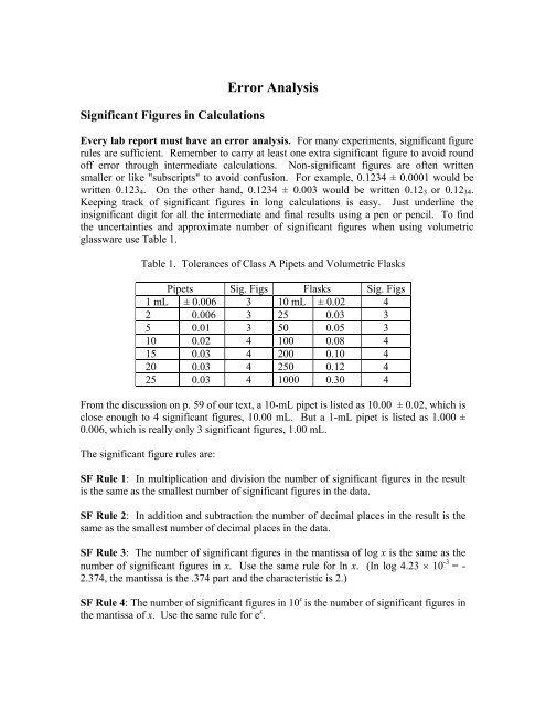
<strong>Significant</strong> <strong>Figures</strong> <strong>in</strong> Calculations<br />
<strong>Error</strong> Analysis<br />
Every lab report must have an error analysis. For many experiments, significant figure<br />
rules are sufficient. Remember to carry at least one extra significant figure to avoid round<br />
<strong>of</strong>f error through <strong>in</strong>termediate calculations. Non-significant figures are <strong>of</strong>ten written<br />
smaller or like "subscripts" to avoid confusion. For example, 0.1234 ± 0.0001 would be<br />
written 0.123 4 . On the other hand, 0.1234 ± 0.003 would be written 0.12 3 or 0.12 34 .<br />
Keep<strong>in</strong>g track <strong>of</strong> significant figures <strong>in</strong> long calculations is easy. Just underl<strong>in</strong>e the<br />
<strong>in</strong>significant digit for all the <strong>in</strong>termediate and f<strong>in</strong>al results us<strong>in</strong>g a pen or pencil. To f<strong>in</strong>d<br />
the uncerta<strong>in</strong>ties and approximate number <strong>of</strong> significant figures when us<strong>in</strong>g volumetric<br />
glassware use Table 1.<br />
Table 1. Tolerances <strong>of</strong> Class A Pipets and Volumetric Flasks<br />
Pipets Sig. Figs Flasks Sig. Figs<br />
1 mL ± 0.006 3 10 mL ± 0.02 4<br />
2 0.006 3 25 0.03 3<br />
5 0.01 3 50 0.05 3<br />
10 0.02 4 100 0.08 4<br />
15 0.03 4 200 0.10 4<br />
20 0.03 4 250 0.12 4<br />
25 0.03 4 1000 0.30 4<br />
From the discussion on p. 59 <strong>of</strong> our text, a 10-mL pipet is listed as 10.00 ± 0.02, which is<br />
close enough to 4 significant figures, 10.00 mL. But a 1-mL pipet is listed as 1.000 ±<br />
0.006, which is really only 3 significant figures, 1.00 mL.<br />
The significant figure rules are:<br />
SF Rule 1: In multiplication and division the number <strong>of</strong> significant figures <strong>in</strong> the result<br />
is the same as the smallest number <strong>of</strong> significant figures <strong>in</strong> the data.<br />
SF Rule 2: In addition and subtraction the number <strong>of</strong> decimal places <strong>in</strong> the result is the<br />
same as the smallest number <strong>of</strong> decimal places <strong>in</strong> the data.<br />
SF Rule 3: The number <strong>of</strong> significant figures <strong>in</strong> the mantissa <strong>of</strong> log x is the same as the<br />
number <strong>of</strong> significant figures <strong>in</strong> x. <strong>Use</strong> the same rule for ln x. (In log 4.23 × 10 -3 = -<br />
2.374, the mantissa is the .374 part and the characteristic is 2.)<br />
SF Rule 4: The number <strong>of</strong> significant figures <strong>in</strong> 10 x is the number <strong>of</strong> significant figures <strong>in</strong><br />
the mantissa <strong>of</strong> x. <strong>Use</strong> the same rule for e x .
Example 1: Concentration Calculations: A solution is made by transferr<strong>in</strong>g 1 mL <strong>of</strong> a<br />
0.1245 3 M solution, us<strong>in</strong>g a volumetric pipet, <strong>in</strong>to a 200-mL volumetric flask. Calculate<br />
the f<strong>in</strong>al concentration.<br />
Solution: The 1-mL volumetric pipet has 3 significant figures; all the other values have<br />
4. The calculations all <strong>in</strong>volve multiplication and division, so the f<strong>in</strong>al answer should be<br />
expressed with 3 significant figures.<br />
1.00 × 0.1245 3 M / 200.0 = 0.000622 6 M = 6.22 × 10 -4 M<br />
Example 2: Logs: The equilibrium constant for a reaction at two different temperatures<br />
is 0.032 2 at 298.2 and 0.47 3 at 353.2 K. Calculate ln(k 2 /k 1 ).<br />
Solution: Both k’s have 2 significant figures, so k 2 /k 1 should also have 2 significant<br />
figures: k 2 /k 1 = 13. 89 . Then us<strong>in</strong>g SF Rule 3 shows that ln k 2 /k 1 should have 2 significant<br />
figures <strong>in</strong> the “mantissa:”<br />
ln k 2 /k 1 = ln 13. 89 = 2.63 1<br />
Example 3: Antilogs: The rate <strong>of</strong> a reaction depends on temperature as ln k = ln A –<br />
E a/ RT. Us<strong>in</strong>g curve fitt<strong>in</strong>g it was found that ln A = 9.87 4 . Calculate A.<br />
87<br />
Solution: The result is e 9.<br />
4<br />
= 1.9427 × 10<br />
4 . The mantissa has only 2 significant figures,<br />
so the result should only have two significant figures (SF Rule 4).<br />
1.9 4 × 10 4 , or just 1.9 × 10 4<br />
Example 4: Antilogs: The rate <strong>of</strong> a reaction depends on temperature as ln k = ln A –<br />
E a /RT. Us<strong>in</strong>g curve fitt<strong>in</strong>g it was found that ln A = 9.87 4 and E a = 28.2 6 kJ/mol. Calculate<br />
k at T = 298.15 K.<br />
Solution: The result for ln k has 2 significant figures: both ln A and E a have 3 significant<br />
figures (SF Rule 1), but the difference has only one past the decimal po<strong>in</strong>t:<br />
ln k = 9.87 4 – 28.2 6 × 10 3 /[(8.314)(298.15)] = 9.87 4 – 11.4 0 = -1.5 266<br />
The mantissa has only 1 significant figure. Then solv<strong>in</strong>g for k and us<strong>in</strong>g SF Rule 4 gives<br />
k = −1<br />
5 266<br />
= 0.217 or f<strong>in</strong>ally just 0.2<br />
e .
<strong>Propagation</strong> <strong>of</strong> <strong>Error</strong>s<br />
<strong>Significant</strong> figure rules are sufficient when you do not have good estimates for the<br />
measurement errors. If you do have good estimates for the measurement errors then a<br />
more careful error analysis based on propagation <strong>of</strong> error rules is appropriate. Least<br />
squares curve fitt<strong>in</strong>g provides very good estimates for uncerta<strong>in</strong>ties. For error analysis<br />
with the slope or <strong>in</strong>tercept from least squares curve fitt<strong>in</strong>g, a little more care is justified<br />
than is provided by significant figure rules. <strong>Use</strong> propagation <strong>of</strong> error rules to f<strong>in</strong>d the<br />
error <strong>in</strong> f<strong>in</strong>al results derived from curve fitt<strong>in</strong>g.<br />
The propagation <strong>of</strong> error rules are listed below. The variance <strong>of</strong> x, (σ x ) 2 , is the square <strong>of</strong><br />
the standard deviation, σ x (an e can also denote the error or uncerta<strong>in</strong>ty and an s the<br />
estimated standard deviation).<br />
Rule 1: Variances add on addition or subtraction. For z = x ± y, (σ z ) 2 = (σ x ) 2 + (σ y ) 2<br />
Rule 2: Relative variances add on multiplication or division. For z = x · y or z = x/y,<br />
2<br />
2<br />
2<br />
⎛ σ<br />
⎛ σ ⎞<br />
z ⎞ ⎛ σ<br />
x ⎞ y<br />
⎜ ⎟ = ⎜ ⎟ +<br />
⎜<br />
⎟<br />
⎝ z ⎠ ⎝ x ⎠ ⎝ y ⎠<br />
Rule 3: The variance <strong>in</strong> ln x is equal to the relative variance <strong>in</strong> x and the variance <strong>in</strong> log x<br />
is the (relative variance <strong>in</strong> x)/(2.303) 2 .<br />
⎛ σ<br />
⎝ x<br />
⎞<br />
2<br />
2 x<br />
For z = ln x, ( σ<br />
z<br />
) = ⎜ ⎟ and for z = log x, s<strong>in</strong>ce ln 10 = 2.303, ( σ<br />
z<br />
)<br />
⎠<br />
2<br />
=<br />
1<br />
( ln10)<br />
⎛ σ<br />
x<br />
⎜<br />
⎝ x<br />
Rule 4: The relative variance <strong>in</strong> e x is equal to the variance <strong>in</strong> x and the relative variance<br />
<strong>in</strong> 10 x is equal to the (variance <strong>in</strong> x)(2.303) 2 .<br />
⎛ σ ⎞<br />
⎜ ⎟<br />
⎝ z ⎠<br />
2<br />
For z = e x z<br />
, ( ) 2<br />
and for z = 10 x z<br />
, = ( ln10) 2<br />
( σ ) 2<br />
=<br />
σ<br />
x<br />
⎛ σ ⎞<br />
⎜ ⎟<br />
⎝ z ⎠<br />
Rule 5: In calculations with only one error term, you can work with standard deviation<br />
<strong>in</strong>stead <strong>of</strong> variance.<br />
Rule 6: The variance <strong>of</strong> an average <strong>of</strong> N numbers, each with variance σ 2 , is σ 2 /N. (The<br />
standard deviation <strong>in</strong> the average improves as √(1/N)).<br />
2<br />
x<br />
2<br />
2<br />
⎞<br />
⎟<br />
⎠<br />
These rules all follow from the general formula from calculus for error propagation<br />
e<br />
2<br />
F<br />
2<br />
⎛ ∂ F ⎞<br />
= ⎜ ⎟<br />
⎝ ∂ x ⎠<br />
2<br />
2 ⎛ ∂ F ⎞<br />
ex<br />
+ ⎜ ⎟<br />
⎝ ∂ y ⎠<br />
2<br />
2 ⎛ ∂ F ⎞<br />
e<br />
y<br />
+ ⎜ ⎟<br />
⎝ ∂ z ⎠<br />
e<br />
2<br />
z<br />
K
where one is calculat<strong>in</strong>g some function F which depends upon experimental quantities x,<br />
y, z, … which have random errors e x , e y , e z , … associated with them (see Appendix C).<br />
These rules are also summarized <strong>in</strong> Table 3-1 <strong>of</strong> the text.<br />
.<br />
Example 5: Subtraction: If Z = A – B with A = 163.455 ± 0.002 and B = 1.34 ± 0.02<br />
calculate Z. F<strong>in</strong>d the uncerta<strong>in</strong>ty <strong>in</strong> the result.<br />
Solution: Work with absolute variances (Rule 1) and note that variances always add (i.e.<br />
the error always builds up):<br />
[variance <strong>in</strong> A = (0.002) 2 ] + [variance <strong>in</strong> B = (0.02) 2 ]<br />
variance <strong>in</strong> result (0.02) 2 => standard deviation = 0.02<br />
Result: (163.455 ± 0.002) – (1.34 ± 0.02) = 162.12 ± 0.02<br />
Example 6: Multiplication: The result <strong>of</strong> an experiment is given by (slope × Cp). Let<br />
slope = 123.2 ± 2.4 and Cp = 4.184 ± 0.031. F<strong>in</strong>d the uncerta<strong>in</strong>ty <strong>in</strong> the result.<br />
Solution: The relative variance <strong>of</strong> the result is the sum <strong>of</strong> the relative variances <strong>of</strong> the<br />
data (Rule 2).<br />
[relative variance <strong>in</strong> slope = (2.4/123.2) 2 = (0.019 48 ) 2 = 3.7 94 × 10 -4 ]<br />
+ [relative variance <strong>in</strong> Cp = (0.031/4.184) 2 = (0.0074 09 ) 2 = 5.4 89 × 10 -5 ]<br />
relative variance <strong>in</strong> product = 4.3 43 × 10 -4<br />
relative standard deviation <strong>in</strong> product = √(4.3 43 × 10 -4 ) = 0.020 84 or 2.0 84 %<br />
Result: (123.2 ± 2.4) × (4.184 ± 0.031) = 515.4 68 ± 2.0 84 % = 515 ± 11
Example 7: Logs: The equilibrium constant for a reaction at two different temperatures<br />
is K 1 = 0.0322 ± 0.0007 at 298.2 and K 2 =0.473 ± 0.006 at 353.2 K. Calculate ln(K 2 /K 1 )<br />
and f<strong>in</strong>d the uncerta<strong>in</strong>ty <strong>in</strong> the result.<br />
Solution: Just like Example 6 the relative variance <strong>in</strong> K 2 /K 1 is the sum <strong>of</strong> the relative<br />
variances:<br />
[relative variance <strong>in</strong> K 2 = (0.0007/0.0322) 2 = (0.02 17 ) 2 = 4. 72 × 10 -4 ]<br />
+ [relative variance <strong>in</strong> K 1 = (0.006/0.473) 2 = (0.01 26 ) 2 = 1. 60 × 10 -4 ]<br />
relative variance <strong>in</strong> K 2 /K 1 = 6. 33 × 10 -4<br />
Us<strong>in</strong>g Rule 3 shows that absolute variance <strong>in</strong> ln K 2 /K 1 is the relative variance <strong>in</strong> K 2 /K 1 .<br />
variance <strong>in</strong> ln K 2 /K 1 = relative variance <strong>in</strong> K 2 /K 1 = 6. 33 × 10 -4<br />
standard deviation <strong>in</strong> result = √(6. 33 × 10 -4 ) = 0.02 51<br />
Result: ln(K 2 /K 1 ) = ln 14.6 89 => 2.687 12 ± 0.02 51 = 2.69 ± 0.03<br />
See Example 2 for the significant figure version <strong>of</strong> this error analysis.<br />
Example 8: Antilogs: The rate <strong>of</strong> a reaction depends on temperature as ln k = ln A –<br />
E a /RT. Us<strong>in</strong>g curve fitt<strong>in</strong>g it was found that ln A = 9.874 ± 0.041. Calculate A and f<strong>in</strong>d<br />
the uncerta<strong>in</strong>ty.<br />
Solution: The result is e 9.874 = 1.94 18 × 10 4 . The relative variance <strong>of</strong> the result is the<br />
absolute variance <strong>of</strong> A (Rule 4):<br />
relative variance <strong>of</strong> e 9.874 = variance <strong>of</strong> A = (0.041) 2 = 1.6 81 × 10 -3<br />
relative standard deviation <strong>in</strong> result = √(1.6 81 × 10 -3 ) = 0.041 00 or 4.1 00 %<br />
Result: 1.94 18 × 10 4 ± 4.1 00 % = (1.94 18 ± 0.079 61 ) × 10 4 = (1.94 ± 0.08) × 10 4<br />
See Example 3 for the significant figure version <strong>of</strong> this error analysis.<br />
Example 9: Multiplication with 'certa<strong>in</strong>' numbers: The result <strong>of</strong> a calculation is (slope ×<br />
R), where R is the gas constant <strong>in</strong> J K -1 mol -1 . Let slope = 1.23 ± 0.02. F<strong>in</strong>d the<br />
uncerta<strong>in</strong>ty <strong>in</strong> the result.<br />
Solution: S<strong>in</strong>ce R is known to several more significant figures than the slope, the<br />
uncerta<strong>in</strong>ty <strong>in</strong> R will add very little to the error <strong>in</strong> the f<strong>in</strong>al result. Therefore, R is 'certa<strong>in</strong>'<br />
for this calculation. Rule 5 applies s<strong>in</strong>ce only the slope is <strong>in</strong> error. Therefore, the error <strong>in</strong><br />
the f<strong>in</strong>al result is then just the standard deviation <strong>in</strong> the slope multiplied by R:<br />
Result: slope × R = 1.23 ± 0.02 × 8.31441 26 = 10.2 26 ± 0.1 66 = 10.2 ± 0.2<br />
Example 10: The Inverse <strong>of</strong> the Slope or Intercept: The result <strong>of</strong> an experiment is the<br />
<strong>in</strong>verse <strong>of</strong> the <strong>in</strong>tercept from a graph, 1/b. Let b = 0.523 ± 0.043. F<strong>in</strong>d the uncerta<strong>in</strong>ty <strong>in</strong><br />
the result.
Solution: The relative variance <strong>in</strong> the result is equal to the relative variance <strong>in</strong> the<br />
<strong>in</strong>tercept (Rule 2). We can also work directly <strong>in</strong> terms <strong>of</strong> standard deviation (Rule 5):<br />
relative standard deviation <strong>in</strong> b = 0.043/0.523 = 0.082 21 or 8.2 21 %<br />
relative standard deviation <strong>of</strong> result = relative standard deviation <strong>in</strong> b = 8.2 21 %<br />
Result: 1/b = 1/0.523 = 1.91 20 ± 8.2 21 % = 1.91 20 ± 0.15 71 = 1.91 ± 0.16<br />
Example 11: Division and Subtraction: The term (1/T 2 – 1/T 1 ) is a very common factor<br />
<strong>in</strong> many equations. For T 1 = 298.2 ± 0.2 K and T 2 = 353.2 ± 0.2 K calculate (1/T 2 – 1/T 1 ).<br />
F<strong>in</strong>d the uncerta<strong>in</strong>ty <strong>in</strong> the result.<br />
Solution: Do not be put <strong>of</strong>f by multi-step problems, just work one step at a time. First,<br />
get the uncerta<strong>in</strong>ty <strong>in</strong> 1/T 2 and 1/T 1 . S<strong>in</strong>ce both <strong>of</strong> these are divisions the relative variance<br />
<strong>of</strong> 1/T is just the relative variance <strong>of</strong> T (Rule 2). Then convert to absolute variance to<br />
calculate the error <strong>in</strong> (1/T 2 – 1/T 1 ) us<strong>in</strong>g Rule 1:<br />
relative variance <strong>in</strong> T 2 = (0.2/353.2) 2 = 3. 20 × 10 -7<br />
relative variance <strong>in</strong> T 1 = (0.2/298.2) 2 = 4. 49 ×10 -7<br />
[variance <strong>in</strong> 1/T 2 = 3.2 × 10 -7 (1/353.2) 2 = 2. 57 × 10 -12 ]<br />
+ [variance <strong>in</strong> 1/T 1 = 4.5 ×10 -7 (1/298.2) 2 = 5. 05 × 10 -12 ]<br />
variance <strong>in</strong> (1/T 2 – 1/T 1 ) = 7. 62 × 10 -12<br />
standard deviation <strong>in</strong> result = √(7. 62 × 10 -12 ) = 2. 76 × 10 -6<br />
Result: -5.221 96 × 10 -4 ± 2. 76 × 10 -6 = (-5.22 ± 0.03) × 10 -4<br />
Example 12: A Multi-Step Problem: An example <strong>of</strong> a more realistic problem is the<br />
temperature dependence <strong>of</strong> the equilibrium constant. We wish to evaluate ΔH, know<strong>in</strong>g<br />
K 1 , K 2 , R, T 1 , and T 2 <strong>in</strong> the equation:<br />
ln(K 2 /K 1 ) = – ΔH/R (1/T 2 – 1/T 1 )<br />
where K 1 = 0.0322 ± 0.0007 at 298.2 and K 2 = 0.473 ± 0.006 at 353.2 K with T = ± 0.2 K<br />
(The same data as <strong>Examples</strong> 7 and 11). F<strong>in</strong>d the uncerta<strong>in</strong>ty <strong>in</strong> the result.<br />
Solution: Solv<strong>in</strong>g for ΔH: ΔH = – 8.31441[ln(K 2 /K 1 )]/(1/T 2 – 1/T 1 ) = 42.78 44 kJ/mol<br />
We already know the uncerta<strong>in</strong>ty <strong>in</strong> ln(K 2 /K 1 ) from Example 7, 2.687 12 ± 0.02 51 , and the<br />
uncerta<strong>in</strong>ty <strong>in</strong> (1/T 2 – 1/T 1 ) from Example 11, (-5.221 96 ± 0.02 76 ) × 10 -4 . R is a certa<strong>in</strong><br />
number. The relative variance <strong>in</strong> ΔH is then just the sum <strong>of</strong> the relative variances:<br />
relative variance ΔH = (0.02 51 /2.687 12 ) 2 + (0.02 76 × 10 -4 / 5.221 96 × 10 -4 ) 2 = 1.1 51 × 10 -4<br />
relative standard deviation <strong>of</strong> ΔH = √(1.1 51 × 10 -4 ) = 0.010 73 or 1.0 73 %<br />
standard deviation <strong>of</strong> ΔH = (0.010 73 )(42.78 44 ) = 0.45 91 kJ/mol<br />
Result: ΔH = 42.78 ± 0.46 => 42.8 ± 0.5 kJ/mol