System identification of non-linear hysteretic systems
System identification of non-linear hysteretic systems
System identification of non-linear hysteretic systems

You also want an ePaper? Increase the reach of your titles
YUMPU automatically turns print PDFs into web optimized ePapers that Google loves.
5 th GRACM International Congress on Computational Mechanics<br />
GRACM 05<br />
Limassol, 29 June – 1 July, 2005<br />
© GRACM<br />
SYSTEM IDENTIFICATION OF NON-LINEAR HYSTERETIC SYSTEMS WITH<br />
APPLICATION TO FRICTION PENDULUM ISOLATION SYSTEMS<br />
Panos C. Dimizas and Vlasis K. Koumousis<br />
Institute <strong>of</strong> Structural Analysis and Aseismic Research<br />
National Technical University <strong>of</strong> Athens<br />
NTUA, Zografou Campus GR-15773, Athens, Greece<br />
e-mail: vkoum@central.ntua.gr, web page: http://users.ntua.gr/vkoum<br />
Keywords: <strong>System</strong> Identification, Hysteresis, Friction Pendulum <strong>System</strong>s, Seismic Isolation.<br />
Abstract. In this work, the parameter <strong>identification</strong> <strong>of</strong> <strong>non</strong>-<strong>linear</strong> dynamical <strong>systems</strong> is presented. More<br />
specifically the <strong>non</strong>-<strong>linear</strong> <strong>hysteretic</strong> behavior <strong>of</strong> seismic isolators modeled by the versatile Bouc-Wen model<br />
such as FPS is determined based on given data. The primal objective <strong>of</strong> this paper is to develop a parametric<br />
<strong>identification</strong> method for the modeling <strong>of</strong> FPS seismic isolator from periodic vibration experimental data. The<br />
estimation <strong>of</strong> the model parameters based on measured data from periodic experiments is implemented using a<br />
time domain method. The Bouc-Wen differential model is adopted to take into account the <strong>hysteretic</strong> frictional<br />
damping <strong>of</strong> the FPS bearings. Then, the parameter <strong>identification</strong> problem is solved using <strong>non</strong><strong>linear</strong> optimization<br />
methods such as the Levenberg-Marquardt algorithm. The <strong>identification</strong> results, <strong>of</strong> the proposed method, are<br />
verified by numerical simulations and the accuracy <strong>of</strong> the identified parameters is verified by comparing the<br />
experimentally measured and the identified time histories.<br />
1 INTRODUCTION<br />
In recent years, the Friction Pendulum <strong>System</strong> (FPS) has become a widely accepted device for seismic<br />
isolation <strong>of</strong> structures. The concept is to isolate the structure from ground shaking during strong earthquake.<br />
Seismic isolation <strong>systems</strong> like the FPS are designed to lengthen the structural period far from the dominant<br />
frequency <strong>of</strong> the ground motion and to dissipate vibration energy during an earthquake. The FPS consists <strong>of</strong> a<br />
spherical stainless steel surface and a slider, covered by a Teflon-based composite material. During severe<br />
ground motion, the slider moves on the spherical surface lifting the structure and dissipating energy by friction<br />
between the spherical surface and the slider.<br />
Friction Pendulum <strong>System</strong>s exhibit <strong>non</strong><strong>linear</strong> inelastic behavior under severe dynamic loading such as<br />
earthquakes. In the case <strong>of</strong> cyclic loading the <strong>non</strong><strong>linear</strong> restoring force <strong>of</strong> such isolators exhibits <strong>hysteretic</strong> loops<br />
and is memory-dependent. It depends not only on the instantaneous deformation, but also on the history <strong>of</strong><br />
deformation. This memory nature makes modeling and analysis more difficult than other <strong>non</strong>-<strong>linear</strong> <strong>systems</strong>. A<br />
widely used model that describes <strong>hysteretic</strong> behavior that belongs to the class <strong>of</strong> endochronic models is that <strong>of</strong><br />
Bouc-Wen [1] . This model consists <strong>of</strong> a system <strong>of</strong> <strong>non</strong><strong>linear</strong> differential equations where the memory-depended<br />
nature <strong>of</strong> hysteresis is taken into account with the use <strong>of</strong> an extra variable. Different values <strong>of</strong> the parameters <strong>of</strong><br />
this model reveal a wide range <strong>of</strong> different mechanical behavior. This accounts for s<strong>of</strong>tening/hardening behavior,<br />
stiffness degradation, strength deterioration, pinching etc. An appropriate choice <strong>of</strong> parameters determined by the<br />
<strong>identification</strong> algorithm on experimental data makes it possible to describe sufficiently the <strong>non</strong>-<strong>linear</strong> dynamic<br />
behavior <strong>of</strong> a <strong>hysteretic</strong> system.<br />
In the past two decades, several researchers have devoted their efforts to identify the parameters <strong>of</strong> the Bouc-<br />
Wen model using experimental data. From a mathematical standpoint, determination <strong>of</strong> the <strong>hysteretic</strong> loop<br />
parameters by <strong>identification</strong> is a problem <strong>of</strong> <strong>non</strong>-<strong>linear</strong> multivariate optimization. In this paper, this problem is<br />
solved using a popular gradient optimization algorithm called the Levenberg-Marquardt method. In section 2, the<br />
versatile Bouc-Wen model is presented to take into account the inelastic behavior <strong>of</strong> the FPS bearings. The time<br />
domain <strong>identification</strong> algorithm is presented in section 3. The effectiveness and accuracy <strong>of</strong> the proposed<br />
algorithm is addressed in section 4 with the aid <strong>of</strong> a numerical study. Finally, this paper concludes with the<br />
presentation <strong>of</strong> <strong>identification</strong> results using the proposed algorithm and a summary <strong>of</strong> the findings in section 5.
2 HYSTERETIC MODEL<br />
Panos C. Dimizas and Vlasis K. Koumousis<br />
2.1 Bouc-Wen <strong>hysteretic</strong> model<br />
In the context <strong>of</strong> a forced single degree <strong>of</strong> freedom <strong>hysteretic</strong> oscillator the equation <strong>of</strong> motion using the Bouc-<br />
Wen model is as follows:<br />
mx ̇̇ + cẋ + akx + (1 − a)<br />
kz = f<br />
(1)<br />
where m, c, k,<br />
f and a are the mass, damping coefficient, stiffness, external excitation and plastic to elastic<br />
stiffness ratio respectively. The <strong>hysteretic</strong> auxiliary variable z , according to the Bouc-Wen model is given by:<br />
The ultimate value <strong>of</strong> z is given by:<br />
( γ β )<br />
n<br />
ż = Aẋ − | z | sign( xz ̇ ) + ẋ<br />
(2)<br />
z<br />
MAX<br />
⎡ A ⎤<br />
= ⎢<br />
β + γ ⎥<br />
⎣ ⎦<br />
1<br />
n<br />
(3)<br />
In the case <strong>of</strong> system <strong>identification</strong>, apart from the mass m that can be measured, all the other parameters <strong>of</strong> the<br />
model are to be identified resulting in the following unknown parameter vector:<br />
[ β γ ] T<br />
p = a k c A n<br />
(4)<br />
2.2 Identification issues and model limitations<br />
The Bouc-Wen model parameters A, β , γ are the one that control the <strong>hysteretic</strong> loop shape, whereas<br />
parameter n affects the smoothness <strong>of</strong> the <strong>hysteretic</strong> curves. A large variety <strong>of</strong> complex <strong>non</strong>-<strong>linear</strong> <strong>hysteretic</strong><br />
dynamic behavior can be represented by the Bouc-Wen model through an appropriate choice <strong>of</strong> these parameters.<br />
Wong et al [2, 3] conducted an extensive study <strong>of</strong> the parameters effect on the response <strong>of</strong> the Bouc-Wen model.<br />
On the other hand, Erlicher and Point [4] proved the constraints that must hold for the Bouc-Wen model<br />
parameters so that it is thermodynamically admissible. Therefore, during Bouc-Wen model <strong>identification</strong>, one<br />
must also take into account the restrictions and constraints regarding the Bouc-Wen model parameters.<br />
Another issue that has to do with the <strong>identification</strong> <strong>of</strong> the Bouc-Wen model is the <strong>non</strong>-smoothness <strong>of</strong> the<br />
<strong>hysteretic</strong> restoring force. The main advantage <strong>of</strong> the Bouc-Wen model is the ability to capture <strong>non</strong>-smooth<br />
dynamic behavior as the sliding <strong>of</strong> an FPS seismic isolator using an analytic mathematical formulation. However,<br />
the implementation <strong>of</strong> <strong>identification</strong> algorithms on rapidly changing dynamical <strong>systems</strong>, such as the FPS<br />
isolators, renders the common <strong>identification</strong> methodologies unable to track them. As claimed by Ching and<br />
Glaser [5] , the reason is that all these <strong>identification</strong> methodologies possess the inherent assumption that the degree<br />
<strong>of</strong> change <strong>of</strong> the dynamical system studied is uniform in time. So, <strong>systems</strong> with frictional slip like the FPS are<br />
difficult to be identified. Additionally, the problem <strong>identification</strong> <strong>of</strong> the Bouc-Wen model becomes harder<br />
because <strong>of</strong> the fact that in certain cases, different combinations <strong>of</strong> some parameters may produce almost identical<br />
<strong>hysteretic</strong> loops [6] .<br />
2.3 Modelling <strong>of</strong> FPS seismic isolators<br />
As explained in the last section, <strong>identification</strong> <strong>of</strong> the seven unknown parameters <strong>of</strong> equation possesses great<br />
difficulties. However, in the case <strong>of</strong> FPS bearings, the <strong>identification</strong> problem can be simplified. The natural<br />
period <strong>of</strong> a FPS bearing is only related to the radius <strong>of</strong> the concave surface R :<br />
T<br />
R<br />
= 2π<br />
(5)<br />
g<br />
where g is the acceleration <strong>of</strong> gravity.<br />
With the aid <strong>of</strong> equation (5), the post yield (sliding) stiffness <strong>of</strong> the FPS can be calculated by:
Panos C. Dimizas and Vlasis K. Koumousis<br />
g<br />
ak = m (6)<br />
R<br />
It is common among researchers [7] to assume that in the case <strong>of</strong> FPS bearings, energy is dissipated by means<br />
<strong>of</strong> frictional sliding <strong>of</strong> the isolator, so one can assume that there is very little or not at all viscous damping:<br />
c ≈ 0<br />
(7)<br />
Finally, the value <strong>of</strong> parameter a usually, in the case <strong>of</strong> FPS isolators, is taken equal to:<br />
Using equation (7), the equation <strong>of</strong> motion <strong>of</strong> the FPS becomes:<br />
a ≈ 0.1<br />
(8)<br />
mx ̇̇ + akx + (1 − a)<br />
kz = f<br />
(9)<br />
where the <strong>hysteretic</strong> auxiliary variable z is given by equation (2).<br />
The post yield stiffness ak can be calculated by equation (6) resulting to the following unknown parameter<br />
vector:<br />
[ β γ ] T<br />
p = A n<br />
(10)<br />
One can see that the unknown parameters were reduced from seven to four and that in the case <strong>of</strong> a periodic<br />
vibration experiment, the <strong>hysteretic</strong> auxiliary variable can be easily measured.<br />
3 TIME DOMAIN PARAMETER ESTIMATION<br />
In the case <strong>of</strong> a periodic vibration test <strong>of</strong> a FPS bearing, both the cyclic excitation f and response x are<br />
measured. One can then evaluate the post yield stiffness ak and the evolution <strong>of</strong> the <strong>hysteretic</strong> auxiliary variable<br />
z using equations (6) and (9) respectively. The evolution <strong>of</strong> ż can then be calculated by numerical differentiation<br />
<strong>of</strong> the variable z. Equation (2) can be rewritten as:<br />
( γ β )<br />
n<br />
D( t) = ż − Aẋ + | z | sign( xz ̇ ) + ẋ<br />
(11)<br />
If the actual force-displacement relation conforms completely to the Bouc-Wen model and p are the true model<br />
parameters, then equation (11) should be equal to zero regardless <strong>of</strong> time t. In fact, equation (11) never<br />
approaches zero due to model errors and measurement noise. Hence, the <strong>identification</strong> problem becomes a <strong>non</strong><strong>linear</strong><br />
optimization one, with equation (11) representing the error residuals. The objective function whose<br />
minimum one seeks, in terms <strong>of</strong> <strong>non</strong>-<strong>linear</strong> least squares, becomes:<br />
1<br />
F p = ∑ D p<br />
(12)<br />
t<br />
( )<br />
2<br />
2<br />
( )<br />
t<br />
1<br />
The resulting <strong>non</strong>-<strong>linear</strong> least-squares optimization problem can be solved using the Levenberg-Marquardt<br />
algorithm [8] . The parameters that minimize the objective function (12) are found by the iteration formula <strong>of</strong> the<br />
algorithm:<br />
t+ 1 t T<br />
1<br />
T<br />
⎡ µ ⎤<br />
−<br />
p = p − ⎣J J + I ⎦ J D<br />
(13)<br />
where J is the Jacobian matrix and µ the Levenberg – Marquardt parameter.<br />
The Jacobian matrix J that is required for the implementation <strong>of</strong> the algorithm can be derived analytically by<br />
the equations:
Panos C. Dimizas and Vlasis K. Koumousis<br />
∂D( t)<br />
= −ẋ<br />
∂A<br />
∂D( t)<br />
= ẋ<br />
| z |<br />
∂β<br />
∂D( t)<br />
n<br />
= ẋ<br />
| z | sign( xz ̇ )<br />
∂γ<br />
n<br />
∂D( t)<br />
n<br />
= ẋ<br />
| z | ln( z ) sign( xz)<br />
+<br />
∂n<br />
( γ ̇ β )<br />
In the time domain implementation <strong>of</strong> the algorithm, the residuals are calculated at each iteration step with the<br />
aid <strong>of</strong> equation (11) using the time series from the periodic vibration experiment. After that, the Jacobian matrix<br />
is calculated analytically using equation (14). Finally, the new parameter values are estimated using the iteration<br />
formula shown in equation (13). In the case where there is a range <strong>of</strong> different periodic vibration tests, the<br />
algorithm is implemented in a similar way, but using as an objective function the sum <strong>of</strong> residuals <strong>of</strong> each<br />
experiment.<br />
The Levenberg-Marquardt algorithm is a popular gradient method for unconstrained optimization. To<br />
improve convergence and stability, one can impose constraints on the algorithm by introducing new parameters<br />
enforced by logistic transformations as Zhang et al. [9] suggest.<br />
4 APPLICATION TO FRICTION PENDULUM SYSTEMS<br />
The <strong>identification</strong> method presented in the previous sections was examined through <strong>identification</strong> <strong>of</strong> FPS<br />
bearings. In order to evaluate the accuracy <strong>of</strong> the <strong>identification</strong> algorithm, a set <strong>of</strong> realistic parameters were used<br />
to numerically generate experimental data. The experimental data were obtained by solving numerically the<br />
system <strong>of</strong> <strong>non</strong>-<strong>linear</strong> differential equations (9) and (2) using a 4 th -5 th order Embedded Runge Kutta method under<br />
sinusoidal excitation f. The Bouc-Wen model parameters used throughout the numerical simulation are<br />
summarized in table 1.<br />
m a k c Α β γ n<br />
1 0.1 10 0 1 0.1 0.9 2<br />
Table 1: Bouc-Wen model parameter values used throughout the numerical simulation<br />
This set <strong>of</strong> parameters yields maximum value for the <strong>hysteretic</strong> auxiliary parameter z<br />
MAX<br />
= 1 and it was<br />
chosen because it is suggested by other researchers [10] for capturing the dynamic behavior <strong>of</strong> FPS seismic<br />
isolators in a sufficient way. According to this set <strong>of</strong> parameters, the natural period <strong>of</strong> such a system is<br />
T = 6.3sec .<br />
To verify the time domain <strong>identification</strong> algorithm, a numerical experiment was conducted using sinusoidal<br />
excitation ( f = 15sin 0.1t<br />
). The amplitude <strong>of</strong> the excitation was chosen so that strong <strong>non</strong><strong>linear</strong>ities and sliding<br />
<strong>of</strong> the isolator was manifested. As claimed by other researchers [11] , the <strong>identification</strong> method gives best results<br />
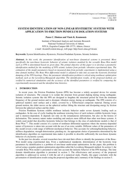
with a few cycles <strong>of</strong> <strong>non</strong>-<strong>linear</strong> response. The <strong>hysteretic</strong> loops and the evolution <strong>of</strong> the <strong>hysteretic</strong> auxiliary<br />
variable z are shown in figure 1 and 2 respectively.<br />
The <strong>identification</strong> method was conducted on the steady state part <strong>of</strong> the experimental data using a two-period<br />
signal. To examine whether the algorithm was sensitive to initial parameter guesses, four sets <strong>of</strong> initial parameter<br />
values were tried. The initial values used are shown in table 2. The results <strong>of</strong> <strong>identification</strong> algorithm are<br />
summarized on table 3 and it becomes evident that the method behaved very well since it managed to converge to<br />
the global minimum <strong>of</strong> the objective function.<br />
Initial Parameter Values Sets<br />
Model Parameters 1 st 2 nd 3 rd 4 th<br />
A 0.1 1 5 10<br />
β 0.1 1 5 10<br />
γ 0.1 1 5 10<br />
n 0.1 1 5 10<br />
Table 2: Different initial parameter values sets.<br />
(14)
Panos C. Dimizas and Vlasis K. Koumousis<br />
Identified parameter using different initial sets<br />
Model Parameters Real 1 st 2 nd 3 rd 4 th<br />
A 1 1.002 1.002 1.002 1.002<br />
β 0.1 0.1076 0.1076 0.1076 0.1076<br />
γ 0.9 0.8944 0.8944 0.8944 0.8944<br />
n 2 1.9962 1.9962 1.9962 1.9962<br />
z 1 1 1 1 1<br />
MAX<br />
Table 3: Identification results.<br />
In order to examine the effect <strong>of</strong> noise on the <strong>identification</strong> accuracy the numerical experimental data were<br />
corrupted with noise:<br />
x( t) = x( t)<br />
+ εr<br />
(15)<br />
where ε represents the signal to noise ratio level and r is a random variable with zero mean and unit<br />
variance. The time series <strong>of</strong> numerically obtained displacement and velocity were corrupted with discrete noise<br />
<strong>of</strong> various levels and the <strong>identification</strong> method was implemented again using various initial conditions. The<br />
results <strong>of</strong> the <strong>identification</strong> method using the second set <strong>of</strong> initial conditions are summarized in table 4.<br />
Identified parameter using different noise levels<br />
Model Parameters Real e=0.001 e= 0.005 e= 0.01 e=0.02<br />
A 1 1.002 1.0095 1.036 1.1542<br />
β 0.1 0.1078 0.1455 0.2591 0.5572<br />
γ 0.9 0.8941 0.8626 0.7721 0.5839<br />
n 2 1.9888 1.8091 1.3876 0.6507<br />
z 1 1.0001 1.0008 1.0033 1.0176<br />
MAX<br />
Table 4: Identification results using noise corrupted data.<br />
It becomes clear from table 4 that the <strong>identification</strong> accuracy is reduced with the increase <strong>of</strong> the level <strong>of</strong> noise.<br />
In the case <strong>of</strong> substantial noise, identified parameter values may be completely different from the real ones. The<br />
most sensitive parameter seems to be n. The values <strong>of</strong> the other parameters seem to deviate from the real ones,<br />
but in a way such that the ultimate value <strong>of</strong> the <strong>hysteretic</strong> variable z is very close to the real one.<br />
Zhang et al. [9] propose the use <strong>of</strong> digital filters in series into the <strong>identification</strong> algorithm for expanding the<br />
capabilities <strong>of</strong> the optimization algorithm. Following their suggestion, the noisy experimental data were filtered<br />
using two digital filters. The first was a median filter and the second was a least-squares lowpass filter also<br />
known as the Savitzky-Golay FIR lowpass filter. The algorithm was implemented for various noise levels and the<br />
results are summarized in table 5.<br />
Identified parameter using different noise levels<br />
Model Parameters Real e=0.01 e= 0.02 e= 0.05 e=0.1<br />
A 1 1.004 1.0037 1.0092 0.9623<br />
β 0.1 0.1064 0.1049 0.1482 0.0793<br />
γ 0.9 0.8946 0.8952 0.8576 0.876<br />
n 2 1.9889 1.9644 1.9212 1.8872<br />
z 1 1.0015 1.0019 1.0018 1.0038<br />
MAX<br />
Table 5: Identification results using digitally filtered data.<br />
A comparison between table 4 and table 5 shows that noise pre-filtering <strong>of</strong> the experimental data expands<br />
significantly the accuracy and effectiveness <strong>of</strong> the proposed <strong>identification</strong> algorithm. A comparison between the<br />
<strong>hysteretic</strong> loops obtained from noisy and noise pre-filtered data is shown in figures 3 and 4.
5 CONCLUSIONS<br />
Panos C. Dimizas and Vlasis K. Koumousis<br />
An <strong>identification</strong> method is proposed for the estimation <strong>of</strong> parameters <strong>of</strong> the Bouc-Wen model based on<br />
experimental data. The <strong>identification</strong> problem is solved using <strong>non</strong><strong>linear</strong> optimization methodologies developed in<br />
the time domain. Parameter estimation was accomplished using the gradient Levenberg-Marquardt method. It<br />
was shown that the <strong>identification</strong> method was able to capture the inelastic dynamic behavior in the case <strong>of</strong><br />
reliable experimental data. From the parametric studies conducted, the method was found to be insensitive to the<br />
initial guesses <strong>of</strong> the parameter values.<br />
The effect <strong>of</strong> noise on the accuracy <strong>of</strong> the method was studied extensively. It was found that the method is<br />
sensitive to noise-corrupted data. As far as the Bouc-Wen model parameters are concerned, the presence <strong>of</strong> noise<br />
seems to play an important role in the final parameter values, especially for the exponential parameter n. It was<br />
also shown that a change in this parameter requires a significant change in the other parameter values in order to<br />
fit the same <strong>hysteretic</strong> loops. However, it was shown that by digital filtering the noisy experimental data, one can<br />
expand the capabilities and the accuracy <strong>of</strong> the <strong>identification</strong> method significantly.<br />
REFERENCES<br />
[1] Wen, Y. K., (1976), “Method <strong>of</strong> random vibration <strong>of</strong> <strong>hysteretic</strong> <strong>systems</strong>” J. Engineering Mechanics Division<br />
102, pp. 249-263.<br />
[2] Wong, C. W., Ni, Y. Q. and Ko, J. M., (1994), “Steady state oscillation <strong>of</strong> <strong>hysteretic</strong> differential model. I:<br />
Response analysis” J. Engineering Mechanics, 120, pp. 2271-2298.<br />
[3] Wong, C. W., Ni, Y. Q. and Ko, J. M., (1994), “Steady state oscillation <strong>of</strong> <strong>hysteretic</strong> differential model. II:<br />
Performance analysis” J. Engineering Mechanics, 120, pp. 2299-2325.<br />
[4] Erlicher, S. and Point, N., (2004), “Thermodynamic admissibility <strong>of</strong> Bouc-Wen type hysteresis models”<br />
Comptes Rendus Mecanique, 332(1), pp. 51-57.<br />
[5] Ching, J. and Glaser, S. D., (2003), “Tracking rapidly changing dynamical <strong>systems</strong> using a <strong>non</strong>-parametric<br />
statistical method based on Wavelets” Earthquake Engineering & Structural Dynamics, 32, pp. 2377-2406.<br />
[6] Ni, Y. Q., Ko, J. M. and Wong, C. W., (1998), “Identification <strong>of</strong> <strong>non</strong>-<strong>linear</strong> <strong>hysteretic</strong> isolators from periodic<br />
vibration tests.” J. Sound and Vibration, 217(4), pp. 737-756.<br />
[7] Nagarajaiah, S. and Constantinou, M. C., (1989), “Non<strong>linear</strong> dynamic analysis <strong>of</strong> three dimensional base<br />
isolated structures (3D-BASIS)” Buffalo, NY, National Center for Earthquake Engineering Research.<br />
[8] Marquardt, D., (1963), “An algorithm for least-squares estimation <strong>of</strong> <strong>non</strong><strong>linear</strong> parameters” SIAM J. Appl.<br />
Math., Vol. 11, pp. 431-441.<br />
[9] Zhang, H., Foliente, G. C., Yang, Y. and Ma, F. (2002), “Parameter <strong>identification</strong> <strong>of</strong> inelastic structures under<br />
dynamic loads.” Earthquake Engineering & Structural Dynamics, 31, pp. 1113-1130.<br />
[10] Constantinou, M. C., Mokha, A. and Reinhorn, A. M., (1990), “Teflon bearings in base isolation II:<br />
Modelling” J. Struct. Engrg. ASCE, 116(2), pp.455-474<br />
[11] Sues, S. T., Mau, S., T., and Wen, Y. K., (1988), “Identification <strong>of</strong> Degrading Hysteretic Restoring Forces”<br />
J. Engrg. Mech., ASCE, 114, pp.833-846.
Panos C. Dimizas and Vlasis K. Koumousis<br />
Figure 1. Hysteresis loops obtained by numerical simulation<br />
Figure 2. Hysteresis loops obtained by numerical simulation
Panos C. Dimizas and Vlasis K. Koumousis<br />
Figure 3. Comparison between hysteresis loops obtained from noisy data and noise pre-filtered data.<br />
Figure 4. Comparison between hysteresis loops obtained from noisy data and noise pre-filtered data.