Run-Time Parallelization of Large FEM Analyses with PERMAS - intes

[NASA’97] 4th National Symposium on Large-Scale Analysis and Design on High-Performance
Computers and Workstations, October 14-17, 1997 in Williamsburg, VA
Run-Time Parallelization of
Large FEM Analyses with PERMAS
1 INTRODUCTION
M. Ast, ∗ R. Fischer, ∗ J. Labarta, ∗∗ H. Manz ∗
∗ INTES Ingenieurgesellschaft für technische Software mbH, Stuttgart, Germany
∗∗ Universitat Politécnica de Catalunya, Barcelona, Spain
The general purpose Finite Element system PERMAS 1 has been extended to
support shared and distributed parallel computer architectures as well as workstation
clusters. The methods used to parallelize this large application software
package are of high generality and have the capability to parallelize all
mathematical operations in a FEM analysis – not only the solver. Utilizing
the existing hyper-matrix data structure for large, sparsely populated matrices,
a programming tool called PTM was introduced that automatically parallelizes
block matrix operations on-the-fly. PTM totally hides parallelization
from higher order algorithms, thus giving the physically oriented expert a virtually
sequential programming environment. An operation graph of sub-matrix
operations is asynchronously build and executed. A clustering algorithm distributes
the work, performing a dynamic load balancing and exploiting data
locality. Furthermore a distributed data management system allows free data
access from each node. The generality of the approach is demonstrated by
some benchmark examples dealing with different types of FEM analyses.
Two major characteristics have been persistent ever
since the FE-Method is being used. Firstly, FE simulations
are CPU time consuming, and secondly, they
are I/O intensive !
The ongoing evolution in the size and complexity of
finite element models shows that the actual available
computer resources are still a limiting factor. The tendency
to produce finer meshes with a higher number of
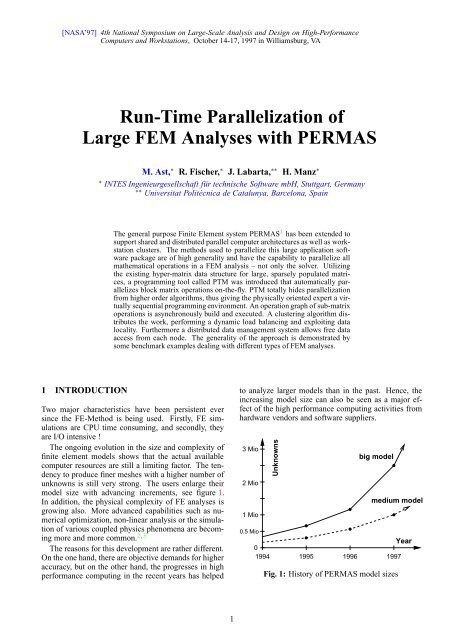
unknowns is still very strong. The users enlarge their
model size with advancing increments, see figure 1.
In addition, the physical complexity of FE analyses is
growing also. More advanced capabilities such as numerical
optimization, non-linear analysis or the simulation
of various coupled physics phenomena are becoming
more and more common. 2, 3
The reasons for this development are rather different.
On the one hand, there are objective demands for higher
accuracy, but on the other hand, the progresses in high
performance computing in the recent years has helped
1
to analyze larger models than in the past. Hence, the
increasing model size can also be seen as a major effect
of the high performance computing activities from
hardware vendors and software suppliers.
3 Mio
2 Mio
1 Mio
Unknowns
big model
medium model
0.5 Mio
Year
0
1994 1995 1996 1997
Fig. 1: History of PERMAS model sizes

Y Z
Since many years the time consuming pre-processing
phase is the most costly part in analysis projects. Therefore
automatic meshing tools were developed in order
to reduce the turnaround times of this phase. Figure 2
shows a typical example for a shell element model
which can be generated from existing geometry in reasonable
time only with at least half-automatic mesh
generators. Automatic mesh generation does, however,
almost inevitable lead to fine meshes with a large number
of unknowns.
Another trend is the increasing number of FEM computations.
For example, the application of automatic
mesh generators also allows even less experienced engineers
to use such methods more and more.
X
Fig. 2: Car body with 130,000 shell elements
(PERMAS at Karmann GmbH, Osnabrück)
Fig. 3: Transmission housing with 311,000 nodes and
963 contacts (PERMAS at ZF Friedrichshafen AG)
2
An impressive example for a today’s nonlinear analysis
can be seen from figure 3. All interior shafts, gears,
and bearings of the transmission housing are modeled
together with excessive contact definitions. Figure 4
shows a coupled simulation. Based on natural modes
and frequencies, a response analysis has to be performed
in the time and frequency domain subsequently.
Fig. 4: Floating ship with fluid-structure interaction
(PERMAS at IRCN, Nantes)
Although computers became much faster in recent
years, it is obvious that hardware speed alone is not
the answer to the demands for high performance computing.
Since single CPU speed enhancements become
more and more difficult, parallelization seems to be the
only solution for further performance speedups. 7
The various forms of parallel algorithms for computational
mechanics are as numerous as the number of
people working on the problem. 4, 5, 6 One obvious approach
is the usage of data parallel programming languages
such as parallel C or HPF. 8, 9 This may be a solution
for new applications designed for these kind of
tools. However for a huge program system with a long
sequential history, rewriting the whole software (or significant
parts of it) is not very practicable.
The most popular way to perform an explicit parallelization
of FE packages is the domain decomposition
approach. 10, 11, 12, 13, 14, 15 In PERMAS, a completely alternative
strategy has been selected. 16
2 PARALLELIZATION STRATEGY
A number of important requirements had to be taken
into account:
• Generality: A general purpose package like PER-
MAS not only has one but several solvers and many
different matrix operations. Hence, a parallelization
of only one solver does not really help. Instead,
a method is required which is able to parallelize
all solvers and matrix operations in a uniform
manner.

• Extendability: The approach must be open to new
developments and has to ensure an easy upgrade of
already existent program parts, i.e. the top solution
procedures shall stay unchanged.
• Maintainability: For both the sequential and parallel
execution, the algorithms and the program versions
have to be the same in order to have a consistent
development of functionalities. An approach is
needed who is as machine independent as possible.
• Portability: Only standard message passing must
be used in order to be able to work on several
machine architectures (like distributed memory,
shared memory or workstation clusters).
• Ease of use: The users should not need additional
knowledge or training to operate with the parallel
code.
Based on the existing program and data structure, not
the well-known domain decomposition but a strategy
based on a mathematical operation graph has been chosen.
Figure 5 gives a basic understanding of the approach
based on a schematic comparison of the two parallelization
methods.
Whereas the parallelism of the domain decomposition
method is achieved through the computation of partial
(sub)models, the parallelism of the PERMAS approach
stems from the computation of Tasks, which are
basic mathematical operations on sub-matrices.
Fig. 5: Different parallelization strategies
3
3 HYPER-MATRIX DATA STRUCTURE
In a Finite Element system, one major objective is the
efficient storage and handling of extremely large but
sparsely populated matrices. In PERMAS this problem
is solved by dividing the matrix in sub-matrices of variable
block size (typically 30∗30 to 128∗128). The complete
matrix, called hyper-matrix, is organized in three
hierarchical levels where levels 2 and 3 contain nothing
but references to the next lower level and level-1
contains the actual data (see figure 6). 17, 18 Of course,
at each level, only sub-matrices containing at least one
non-zero element are stored and processed. Moreover,
on level-1 only the rectangular area of real non-zeros
within that sub-matrix is actually stored.
sym.
n
3
Numeric
Array
(window)
Level 2
Submatrix
n
1
m
Level 3 Matrix
Highest Level
m
m
1
3
2
n
2
Level 1 Submatrix
Lowest Level (paragraph)
Fig. 6: The hyper-matrix data structure
A hyper-matrix operation can be viewed as a stream
of basic block operations on sub-matrices, e.g. a
multiply-add of two level-1 matrices. One major advantage
of this scheme is the high granularity of operations
and the fact that a basic operation typically requires
2∗n 3 floating point operations but only 3∗n 2 memory
accesses. The data structure is simple and hence easily
understood by the programmers. The overhead for
administration of the sub-matrices is small compared to
the basic operations. The typical block size can easily
be adapted to the actual matrix sparsity and hardware
environment, e.g. to optimize vector length or
I/O record size. With respect to parallelization it is
worthwhile to mention that all basic operations on submatrices
are of similar length, i.e. need the same order
of time magnitude for execution.

4 PARALLEL TASK MANAGER
Corresponding to the 3-level data structure all hypermatrix
algorithms are organized in 3 well separated program
layers: Two logical layers working only on addresses
and one numerical layer – usually just a cap to
a standard BLAS routine.
Fig. 7: Parallel Task Manager
For parallelization, a new software layer called the
Parallel Task Manager (PTM) 19 was introduced, see figure
7. PTM offers a complete set of functions for the
traversal of hyper-matrices. These new functions replace
all calls previously made to the sequential data
base manager. A PERMAS programmer implementing
a hyper-matrix algorithm will call PTM to ask for
the existence and properties of particular sub-matrices.
Based on this information he can organize the level 3
and 2 loops just as before – in fact the level 3 and 2
program structure stays unchanged and the call replacements
are quite easy, because the new functions have
similar names and arguments as the old data base calls.
Finally, instead of directly calling a numerical level-1
routine, the programmer passes a task request to PTM.
Each task is defined by a certain opcode (i.e. an identifier
for the level-1 routine to be called) and a reference
to the level-1 sub-matrices to be used. After copying
the task request in an internal buffer PTM immediately
returns control to the calling layer. The task execution
will then be done asynchronously on a node and in a
sequence controlled by PTM.
Inside PTM the graph of sub-matrix operations is
asynchronously build and executed, see figure 8. The
data dependencies are resolved by a graph generator,
which works in a dynamic way according to the actual
loops on the sparse matrix structure. A separate clustering
algorithm collects basic mathematical operations
into packages to be sent. Subsequently, the scheduler is
4
responsible to distribute the tasks to the different nodes
for execution (using MPI). 20 Taking into account the
execution times of completed tasks the scheduler also
ensures a dynamic load balancing – thus adapting itself
to the current load of each node and avoiding bottlenecks
in data distribution.
The problem of finding the optimal schedule of a
number of interdependent tasks is NP complete like the
ordering problem of a sequential graph. Therefore a
number of heuristics have been developed to find reasonable
schedules in affordable computing times. 21, 22
Level-2
address
matrices
Graph
Clusterer
Scheduler
MPI
Executor
Level-1
matrices
*
-
+
node 1
hyper-matrix algorithm
task (opcode + operand address)
node 2
data dependency
node 3 node 4
Fig. 8: Asynchronous generation
and execution of tasks
Running PERMAS on a sequential machine, PTM
executes these basic operations in the same control flow
as if the original functions had been called directly. This
means that we can use the same program version for
both sequential and parallel runs.
The most important aspect of this approach is the
fact that all details of parallel computing are completely
handled inside the tools and hidden from the developer
implementing a new hyper-matrix operation. This allows
the adoption of the PERMAS program to future
hardware architectures without having to change large
parts of the code. The effort in such developments is
hence protected against hardware changes. Moreover,
it is possible to improve the performance-critical parts
like the clustering and scheduling mechanism without
changing any higher order algorithms.

In a parallel environment, the task execution is performed
on the basis of a host-node concept. The host
has only control functionality and executes all of the
sequential program parts, whereas the nodes are executing
all basic numerical operations of a parallel hypermatrix
algorithm, figure 9. With respect to communication
bandwidth it is important to note that a typical task
definition requires less than 70 bytes and that several
task clusters are sent at once in order to minimize the
overall time needed for message startup.
PERMAS PERMAS
Node
Node
PERMAS
PERMAS
Node Node
PERMAS
Node
PERMAS
Disk Disk Disk
Disk Disk
Host
PERMAS
Node
Disk Disk
Disk
Disk
Fig. 9: Centralized Task Control
5 DISTRIBUTED DATA BASE
PERMAS
Node
According to the new needs, the central data base system
had to be upgraded too. A new, Distributed Data
base Management System (DDMS) was introduced,
that controls all data traffic from, and to, the direct access
files of the physically distributed data base (above
DDMS the data base is a logical unity with global references),
see figure 10. One instance of DDMS runs on
each node including the host – regardless of whether a
node has own disks or not. For node-local I/Os DDMS
handles the direct I/O to the local files. In addition it
manages the network traffic due to remote data requests.
Thus DDMS allows free data access from each node,
exploiting the local cache and I/O channels of all nodes.
Unlike the short task messages, the level-1 operands
handled by DDMS have typical sizes of about 128
kbytes. Therefore the distributed characteristic and the
ability to handle node to node communication also ensures
that the host will not become the communication
or administration bottleneck (as it would be with a centralized
data base).
Disk
Disk
5
Due to the asynchronity, the integrity of data has to be
guaranteed. This is realized by a monotonously increasing
version number for task operands, the producer task
identifier (PTI). Each level-1 matrix owes its own PTI,
which is also stored in the referring level-2 matrices.
Each modification changes the PTI and a change is possible
only for one task at a time. With this paradigm the
data traffic can be minimized and possible deadlocks
are avoided.
Node
DDMS
Node
DDMS
Node
DDMS
Host
DDMS
Node
DDMS
Node
DDMS
Node
DDMS
Node
DDMS
Disk Disk Disk
Disk Disk
6 IN PRACTICE
Disk Disk
Disk
Disk
Fig. 10: Distributed Data Base
Management System
Above PTM the parallel and sequential code is identical.
There is only one program version for sequential
and parallel machine architectures. The basic program
structure and programming style of the software development
team can stay unchanged – an essential item
for the code owner’s investments in past and future.
Another advantage is the separation of work fields between
algorithmic oriented specialists and parallelization
experts. The experience of the software developers
show that a functional splitting of work areas always
pays off in terms of productivity, code efficiency and
last but not least stability. In PERMAS this separation
is clearly reflected by different programming levels for
machine, parallelization, algorithmic and physical experts,
see figure 11. Furthermore a single program version
keeps the maintenance simple. There is only one
source code to handle and the quality assurance of the
sequential version is applicable to parallel runs without
change. Again, this is an important point for an industrial
software vendor (who often spends more money on
maintaining than developing a program).
Disk
Disk

Also the end user benefits from this run-time parallelization.
Apart from faster execution times (and
maybe access to more memory and disks) the user’s
daily working environment does not change. No additional
knowledge is necessary and no extra work is
required (e.g. no special mesh partitioning). The program
releases are consistent in the way that the parallel
’version’ offers identical functionality as the sequential
one (indeed it’s the same binary). Moreover,
because a sequential and a parallel run use the same
algorithms, the sequence of operations remains also unchanged.
This gives identical results independent of the
number of computing nodes actually used. This even
offers the possibility to choose the number of nodes by
the system administrator according to a global view of
available computing resources. The user does not have
to care about parallelization – for him there is no difference
between one faster or just more CPUs.
7 BENCHMARKS
All of the following benchmarks have been performed
on an IBM SP-2 (except one specially mentioned), thus
reflecting the behavior of a distributed memory architecture.
All models have been calculated using the direct
solver, since this is still the fastest solver for the
sequential case. This ensures a realistic comparison of
run times.
Compared to present-day mesh sizes the benchmark
models are of medium size only. This is due to various
reasons: First the benchmarks were selected at start
of the parallelization project, thus reflecting the problem
situation in 1994. Second, getting real upto-date
industrial benchmarks for publications is not easy. On
the other hand parallelization rates on larger problems
are usually better, so smaller models are more appropriate
to show possible limitations of the underlying parallelization
strategy.
✏✏
Sequential or parallel hardware (distributed/shared)
✏
✏
✘ Program interface for automatic run-time parallelization
✘ ✘
✥
✥
✥ Basic hyper-matrix algorithms
✭✭ ✭✭
PERMAS FEM system
Fig. 11: PERMAS Program layers
6
Fig. 12: Crank Housing
Fig. 12 (a): Crank Housing, Static Analysis

X
Z
Y
Fig. 13: Methane Carrier
Fig. 13 (a): Methane Carrier, Static Analysis
Fig. 13 (b): Methane Carrier, Dynamic Analysis
7
Z
Y
X
Fig. 14: Artificial Cube (scalable test case)
Fig. 14 (a): Artificial Cube, Cholesky Decomposition
Fig. 15: Contact Analysis of a Motor Piston

Fig. 16: Electromagnetic Wave Propagation of a Box
Fig. 17: Casting Carrier, Static Analysis on SGI
A static analysis of the crank housing shows a reasonable
scalability up to 16 nodes, figure 12 (a). Figure
13 (a) and 13 (b) display two different type of analysis
for the methane carrier. For a static run of this small
model, the solver part itself is less than 50 % of the total
elapsed time already. For the dynamic job the cholesky
decomposition is almost negligible. This demonstrates
that it is not sufficient to parallelize just the solver part.
Also from figure 13 (b) it can be seen that the run-time
parallelization of PTM works for the whole application.
In order to investigate the influence of the model size
an artificial test case was created, figure 14 and 14 (a).
Apart from minor improvements for the larger model,
it can be seen that the parallelism exploited by PTM is
basically independent of the problem size.
Figure 15 present the elapsed times for a non-linear
analysis, whilst figure 16 show the numbers achieved
for the simulation of electromagnetic phenomena. Finally
figure 17 gives an instance for a parallel job on a
shared memory machine.
8
8 CONCLUSIONS
The generality of the parallelization approach has been
presented not only from conceptual but also from the
application point of view. As shown by the examples,
parallelization is also beneficial for medium size models.
The PTM programming interface offers a general
toolbox for automatic parallelization of initially sequential
hyper-matrix algorithms, enabling also unexperienced
programmers to write parallel algorithms.
With this approach, the number of CPUs used for
an analysis becomes a mere performance parameter as
it should be the case. The parallel PERMAS version
may be used without additional know-how and there is
a guarantee of a consistent program evolution for both
the sequential and the parallel version. This is a prerequisite
for a protection of the investments made by the
software supplier. Moreover this is a basic requirement
for a reliable usage on the customer’s side.
Up to now only basic work was done with emphasis
on a clean structure of the software. In order to improve
the scalability of the code and to fully exploit the potential
of the parallelization approach, further development
is needed. However, global tuning can be performed
without changing the PTM interface. This means that
current and future PERMAS procedures will automatically
benefit from any improvement made in this field.
ACKNOWLEDGEMENT
The work reported in this paper is supported by
the European Comission under the ESPRIT projects
PERMPAR 23 and PARMAT. 24
REFERENCES
1. PERMAS: User’s Reference Manual, INTES Publication
No. 450, Rev. D, Stuttgart, 1997. 1
2. CISPAR: Open interface for coupling of industrial simulation
codes on parallel systems, Esprit project 20161,
World Wide Web address: http://www.pallas.de/cispar/. 1
3. Löhner, R., Yang, C., Cebral, J., Baum, J.D., Luo, H.,
Pelessone, D. and Charman, C., Fluid Structure Interaction
Using a Loose Coupling Algorithm and Adaptive Unstructured
Grids, AIAA Paper 95-2259, 1995. 1
4. Noor, A.K., Parallel processing in finite element structural
analysis, Parallel Computations and Their Impact on Mechanics,
ASME, 1987, pp.253-277. 2
5. Ortega, J., Voigt, R., Romine, C., A bibliography on parallel
and vector numerical algorithms, NASA Contractor
Report 181764, ICASE Interim Report 6, 1988. 2
6. White, D.W., Abel, J.F., Bibliography on finite elements
and supercomputing, Commun. Applied Numeric Methods,
4, 1988, pp.279-294. 2
7. Topping, B.H.V., Khan, A.I., Parallel Finite Element
Computations, Saxe-Coburg Publications, Edinburgh,
UK, 1996. 2

8. Wilson, G.V., Lu, P., Stroustrup, B., Parallel Programming
Using C++, MIT Press, Cambridge, MA, 1996. 2
9. Perrin, G.-R., Darte, E., The Data Parallel Programming
Model, Lecture Notes in Computer Science, Vol. 1132,
Springer, Berlin, 1996. 2
10. Farhat, C., Roux, F.-X., Implicit parallel processing
in structural mechanics, Computational Mechanics Advances,
1994, 2(1), pp.1-124. 2
11. Topping, B.H.V., Sziveri, J., Parallel Sub-domain Generation
Method, Developments in Computational Techniques
for Structural Engineering, Civil-Comp Press, Edinburgh,
UK, 1995, pp.449-457. 2
12. Walshaw, C., Cross, M., Everett, M., Mesh partitioning
and load-balancing for distributed memory parallel systems,
Proc. Parallel & Distributed Computing for Computational
Mechanics, Lochinver, Scotland, 1997. 2
13. Liu, J.W.H., The Multifrontal Method for Sparse Matrix
Solution: Theory and Practice, SIAM Review, 34, 1992,
pp.82-109. 2
14. PARASOL: An Integrated Programming Environment for
Parallel Sparse Matrix Solvers, Esprit 4, World Wide Web
address: http://www.genias.de/parasol/. 2
15. Pothen, A., Rothberg, E., Simon, H.D., Wang, L., Parallel
Sparse Cholesky Factorization with Spectral Nested Dissection
Ordering, NAS Technical Report RNR-94-011,
1994. 2
16. Ast, M., Labarta, J., Manz, H., Pérez, A., Schulz and
U., Solé, J., A General Approach for an Automatic Parallelization
Applied to the Finite Element Code PERMAS,
Proceedings of the HPCN Conference, Springer, 1995. 2
9
17. Braun, K.A., et. al., Some Hypermatrix algorithms in Linear
Algebra, Lecture Notes in Economics and Mathematical
Systems, Vol. 134, Springer, Berlin, 1981. 3
18. Rothberg, E., Gupta, A., An Efficient Block-Oriented Approach
to Parallel Sparse Cholesky Factorization, SIAM
Journal of Scientific Computing, 15, 1994, pp.1413-1439.
3
19. Ast, M., Labarta, J., Manz, H., Pérez, A., Schulz, U. and
Solé, J., The Parallelization of PERMAS, Conference on
Spacecraft Structures Materials & Mechanical Testing,
ESA, 1996. 4
20. Snir, M., Otto, S.W., Dongarra, J., MPI: The Complete
Reference, MIT Press, Cambridge, MA, 1996. 4
21. Ast, M., Jerez, T., Labarta, J., Manz, H., Pérez, A.,
Schulz, U. and Solé, J., Runtime Parallelization of the
Finite Element Code PERMAS, International Journal of
Supercomputer Applications and High Performance Computing,
1997, 11(4), pp.328-335. 4
22. El-Rewini, H., Lewis, T., Ali, H.H., Task Scheduling in
Parallel and Distributed Systems, Prentice-Hall, 1994. 4
23. PERMPAR: Implementation of the General Purpose Finite
Element Code PERMAS on High Parallel Computer
Systems, EUROPORT-1, World Wide Web address:
http://www.gmd.de/SCAI/europort-1/C2.HTM. 8
24. PARMAT: Efficient Handling of Large Matrices on
High Parallel Computer Systems in the PERMAS
Code, Esprit project 22740, World Wide Web address:
http://www.intes.de/parmat/. 8