Magara, T., Shibata, K., & Yokoyama, T. 1997, ApJ, 487, 437

THE ASTROPHYSICAL JOURNAL, 487:437È446, 1997 September 20 

( 1997. The American Astronomical Society. All rights reserved. Printed in U.S.A. 

EVOLUTION OF ERUPTIVE FLARES. I. PLASMOID DYNAMICS IN ERUPTIVE FLARES 

TETSUYA MAGARA,1 KAZUNARI SHIBATA,2 AND TAKAAKI YOKOYAMA2 

Received 1996 December 31; accepted 1997 April 15 

ABSTRACT 

We investigate the resistive processes of plasmoid dynamics in eruptive Ñares by performing 2.5- 

dimensional resistive MHD numerical simulations. We start with a linear force-free Ðeld arcade and 

impose the localized resistive perturbation on the symmetry axis of the arcade. Then the magnetic Ðelds 

begin to dissipate, producing inÑows toward this region. These inÑows make the magnetic Ðelds convex 

to the symmetry axis and hence a neutral point is formed on this axis, leading to a formation of a 

magnetic island around the symmetry axis. At the Ðrst stage, the magnetic island slowly rises by the 

upÑow produced by the initial resistive perturbation. Then, once the anomalous resistivity sets in, the 

magnetic island begins to be accelerated. This acceleration stops after the fast MHD shock is formed at 

the bottom of the magnetic island, which implies that the upÑow around the central part of the magnetic 

island is no longer strong. These three stages in the evolution of the plasmoid are conÐrmed to exist in 

the observational results. Moreover, a time lag between the start time when the magnetic island begins 

to be accelerated and the peak time of the neutral-point electric Ðeld can be explained by the inhibition 

of magnetic reconnection by the perpendicular magnetic Ðeld. We also study the di†erence of the initial 

rise motion of the plasmoid between the simulation results and the observational ones, and we conclude 

that, in actual situations, the initial resistive perturbation proceeds very weakly and at many positions 

inside the arcade. 

Subject headings: MHD È Sun: corona È Sun: Ñares È Sun: magnetic Ðelds 

1. INTRODUCTION 

We can observe many activities in the outer atmosphere 

of the Sun. Solar Ñares are one of the most popular active 

phenomena and hence have been so attractive to both theorists 

and observers that much work has been done with 

these objects. Solar Ñares are highly energetic and complicated 

phenomena in which mass eruptions occur, energetic 

particles are generated, and soft or hard X-rays are radiated. 

In this paper, we study the dynamics of mass eruptions 

associated with solar Ñares, which are sometimes called 

plasmoid eruptions or Ðlament eruptions (observed in Ha). 

Theoretically, these eruptive phenomena have been considered 

to be related to an instability or a loss of equilibrium 

of the coronal magnetic Ðeld. Since the magnetic 

force is much stronger than both the gas pressure and the 

gravity force in the corona, coronal structures are mainly 

controlled by the magnetic Ðeld. Therefore, unless a magnetically 

driven event occurs, the coronal structures evolve 

in a series of quasi-static states, but once an instability 

develops or a loss of equilibrium is achieved, they no longer 

stay in a static state and enter on a dynamical stage. This 

scenario has made it important to study the stabilities and 

natures of the equilibrium conÐgurations of the coronal 

magnetic Ðeld. Zweibel (1981, 1982) investigated the stabilities 

of two-dimensional magnetohydrostatic conÐgurations. 

Cargill, Hood, & Migliuolo (1986), Velli & Hood 

(1986), and Hood & Anzer (1987) studied the MHD stabilities 

of the cylindrically symmetric magnetic arcades. 

Viscous e†ect was discussed by van der Linden, Goossens, 

& Hood (1988) and Bogaert & Goossens (1991). 

Zwingmann (1987) showed a series of equilibria of the 

coronal magnetic Ðeld and explained the onset conditions 

for the eruptive phenomena, which were reconsidered by 

1 Department of Astronomy, Faculty of Science, Kyoto University, 

Sakyo-ku, Kyoto 606-01, Japan; magara=kusastro.kyoto-u.ac.jp. 

2 National Astronomical Observatory, Mitaka, Tokyo 181, Japan. 

437 

Platt & Neukirch (1994). Priest (1988) and Steele et al. 

(1989) discussed a loss of equilibrium from the viewpoint of 

CME (coronal mass ejection). Forbes, Priest, & Isenberg 

(1994) estimated the amount of released energy when a loss 

of equilibrium occurs. An approach to this kind of problem 

by using the complex analyses is found in Priest & Forbes 

(1990) and Forbes (1990), for example. 

Recently, the rapid development of computers enabled us 

to trace the temporal evolution of the coronal magnetic 

Ðeld directly by means of numerical simulations. Such work 

is found in Mikic, Barnes, & Schnack (1988), Biskamp & 

Welter (1989), Finn, Guzdar, & Chen (1992), Inhester, Birn, 

& Hesse (1992), Kusano, Suzuki, & Nishikawa (1995), Choe 

& Lee (1996), for example. These papers studied how the 

coronal magnetic Ðeld evolved under those situations where 

the shearing or converging motion was imposed in the 

photosphere. 

Turning to the observations, the satellite Yohkoh has 

brought us many intriguing data of the corona since its 

launch in 1991 August (Masuda 1994; Sakao 1994; Hara 

1996). These data are of good quality, so that they can be 

used to conÐrm the preproposed theories of several solar 

phenomena, for example, the reconnection model of solar 

Ñares (Tsuneta et al. 1992; Magara et al. 1996), as well as to 

propose some new theoretical predictions (Shibata et al. 

1994, 1995). As for the plasmoid eruptions, Ohyama & 

Shibata (1997) analyzed the time-varying behavior of the 

plasmoids in detail and clariÐed their dynamical natures. 

The aim of our paper is to understand theoretically what is 

the basic mechanism working in the plasmoid eruption by 

taking into account some new results obtained by Yohkoh. 

For this purpose, we perform 2.5-dimensional resistive 

MHD simulations and compare the simulation results with 

the observational ones. 

Basic formulations are in the next section. Main results 

are presented in ° 3, and ° 4 is used to mention the observational 

results. In ° 5 we discuss both the obtained results

438 MAGARA, SHIBATA, & YOKOYAMA Vol. 487 

and the related problems and give our conclusions. The 

Ðnal section is devoted to summary. 

2. BASIC FORMULATIONS 

2.1. Basic Equations 

We consider the magnetized atmosphere composed of 

both the magnetic Ðeld and the ideal gas. The e†ect of 

the gravity is neglected for simplicity. Using the Cartesian 

coordinates, the basic equations are 

Lo 

] $ Æ (o¿) \ 0 , (1) 

Lt 

o CL¿ Æ$)¿D Lt ] (¿ \[$P] 1 ($ÂB)ÂB , (2) 

4n 

B AP 

] (¿ Æ$) 

BD g \ 

oc 

c [ 1 

C L 

Lt 

AP 

oc 

oc 

o $ ÂBo2 , (3) 

4n 

LB 

\ $ Â (¿ ÂB)[$Â(g$ÂB) , (4) 

Lt 

P \ oRT 

k . (5) 

In addition, we use $ Æ B \ 0 as an initial condition for 

equation (4). Here all the symbols, such as P, o, T , ¿, and B, 

have their usual meanings, c is the adiabatic index, R is the 

gas constant, k is the mean molecular weight, and g is the 

magnetic di†usivity. All physical values are dependent on 

both the x and z coordinates, but constant along the y- 

coordinate. In practice, calculations are performed for the 

nondimensional values normalized by some particular 

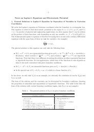
units. These units are summarized in Table 1. 

2.2. Initial ConÐguration 

Initially we assume a linear force-free Ðeld described by 

B x 

\[ 2L 

nH B 0 cos A n 

2L xB e~z@H , (6) 

S A B \[ 1[ A2L B2 B0 cos n xB e~z@H , (7) 

y nH 2L 

B z 

\ B 0 

sin A n 

2L xB e~z@H , (8) 

where L is the horizontal scale length and is taken as the 

normalized length unit (L \ 1.0); H means the vertical scale 

TABLE 1 

UNITS FOR NORMALIZATION 

Physical Values Normalization Units Typical Values 

Length ..................... La 5000 (km) 

Velocity .................... C b 300 (km s~1) 

S0 

Time ........................ L/C 20 (s) 

S0 

Density ..................... o 10~14 (g cm~3) 

0 

Pressure .................... o C2 10 (dyne cm~2) 

Temperature ............... kC 0 

2 S0 

/cR 3 ] 106 (K) 

Magnetic Field ............ (8no S0 

C2 /cb )1@2 8 ] 102 (G) 

Electric Field .............. C (8no 0 S0 

C2 0 

/cb )1@2/c 2 ] 104 (V m~1) 

Magnetic Di†usivity ...... C S0 

L 0 S0 0 

5 ] 1016 (cm2 s~1) 

S0 

NOTE.ÈThe parameters o , T , and C are taken to be the coronal 

values in the active region. c, 0 

k, b 0 

, R, and S0 

c are the adiabatic index, the 

mean molecular weight, the plasma 0 

beta, the gas constant, and the speed of 

light, respectively. 

a L is a half-length between the footpoints of a loop. 

b C is the adiabatic sound velocity deÐned by C 4 (cRT /k)1@2. 

S0 

S0 0 

height of the magnetic Ðeld. For the present study, H ranges 

from 2L /n to O, where H \ 2L /n corresponds to the potential 

Ðeld and H \ O corresponds to the open Ðeld. Usually, 

a linear force-free Ðeld is characterized by a constant 

parameter a, where 

$ ÂB\aB , (9) 

and this value is described by a \ [(n/2L )2[(1/H)2]1@2 in 

our formulation. Therefore, a ranges from 0 (potential Ðeld) 

to n/2L (open Ðeld). A linear force-free Ðeld is the lowest 

energy state for the given boundary conditions with prescribed 

helicity (see Heyvaerts & Priest 1984), but in reality 

the coronal magnetic Ðeld is not always considered to be in 

this state (Schmieder et al. 1996). This is because the relaxation 

time to this state is not so short as the dynamical time 

(see Browning & Priest 1986). However, in the present study 

we start with this state for simplicity. 

The gas pressure P is uniform (P \ P ), and the ratio of 

this to the magnetic pressure is deÐned 0 

as b 4 8nP /B2 

(plasma b). The gas density o is uniform (o \ o ) except 0 

in 

the bottom region where it is 10 times higher 0 

than elsewhere. 

This region is modeled on the massive layers of 

the solar atmosphere, such as the chromosphere and the 

photosphere. Therefore, the gas pressure and density are 

expressed by 

P \ P 0 

, (10) 

o 

\ 4.5Mtanh [[50(z [ 0.1)] ] 1N ] 1 , (11) 

o 0 

respectively. Plasma b is also expressed by 

b \ P 0 

(B2/8n) \ P 0 

(B2/8n)e~(2z@H) \ b e(2z@H) . (12) 

0 0 

In the present study, we adopt b \ 0.2, c \ 5/3, P \ 1/c, 

0 0 

o \ 1, and B \ (8nP /b )1@2 \ (8n/cb )1@2. From now on, 

0 0 0 0 0 

all physical values presented in this paper are normalized by 

the units in Table 1. 

Finally, the temperature is deÐned by 

in the nondimensional form. 

T \ c P o , (13) 

2.3. Boundary Conditions 

Figure 1 illustrates the domain of the present numerical 

simulation. This Ðgure also shows the initial conÐguration 

of the magnetic Ðeld lines projected onto the (x, z) plane. We 

set a free boundary condition at the upper boundary (at 

z \ 40), 

LB x 

Lz \ LB y 

Lz \ Lv x 

Lz \ Lv y 

Lz \ Lv z 

Lz \ LP 

Lz \ 0, $ÆB\0, (14) 

and antisymmetric boundary conditions both along the 

z-axis (at x \ 0) and along the side boundary (at x \ 8), 

v x 

\ v y 

\ B z 

\ Lv z 

Lx \ LB x 

Lx \ LB y 

Lx \ LP 

Lx \ Lo 

Lx \ 0 , (15)

No. 1, 1997 EVOLUTION OF ERUPTIVE FLARES. I. 439 

FIG. 1.ÈInitial conÐguration of the present numerical simulation. Contours 

indicate magnetic Ðeld lines projected onto the (x, z) planes. The dark 

region at the bottom is a high-density region modeled on the massive 

atmosphere, such as the chromosphere and the photosphere. 

and a rigid boundary condition for the lower boundary (at 

z \ 0), 

v \ v \ Lv x 

y z Lz \ LB x 

Lz \ LB y 

Lz \ LB z 

Lz \ LP 

Lz \ Lo 

Lz \ 0 , (16) 

respectively. For the actual calculations, we use the modi- 

Ðed Lax-Wendro† method developed by Shibata and 

Yokoyama (see Shibata et al. 1989; Yokoyama 1995) and 

solve the equations only over a half domain (0 ¹ x ¹ 8), 

assuming a symmetry at x \ 0. The numbers of the mesh 

points are (N ] N ) \ (160 ] 200), where the mesh points 

are distributed x 

uniformly z 

in both of the x and z directions 

and hence the grid size is (*x, *z) \ (0.05, 0.2). 

Although multiple arcades exist in the calculated region, 

our attention is concentrated only on the central one 

(0 ¹ x ¹ 1). The other ones are set in order to make a 

smooth boundary condition at x \ 1. That is, if we set the 

free boundary condition at x \ 1, the e†ect of the resultant 

numerical Ñows would not be negligible. From this point of 

view, the initial perturbations are assigned to the central 

arcade alone (see below), and we investigate this arcadeÏs 

evolution. 

2.4. Initial Perturbations 

Initially, the di†usivity coefficient is set to be g \ 0 everywhere, 

except in a narrow region of [x2](z[h)2]1@2 ¹ r, 

in which g \ g is assigned for a Ðnite time (0 ¹ t ¹ 2). 

Here g is the normalized init 

value and deÐned as the reciprocal 

of the modiÐed magnetic Reynolds number R (4C L /g). 

m s 

Values h and r are those parameters which determine the 

height and radius of the initially perturbed region. In the 

present study, we take various models having di†erent 

values of such parameters as g , h, and r. These models are 

init 

summarized in Table 2. As far as the radius r is concerned, 

all models have r ¹ 0.9, which is because we focus our concentration 

on the central arcade. Model r1Èr4 and model 

g1Èg3 are characterized by the radius r and initially assigned 

resistivity g , respectively. These models are used 

init 

in order to investigate how the natures of the initially perturbed 

region a†ect the subsequent evolution of the system 

(see ° 3.3). Model H1ÈH4 are di†erent with each other in 

their vertical scale heights. Model M, unlike those models 

mentioned above, has four distinct initially perturbed 

regions rather than a single perturbed region, which are all 

distributed along the z-axis. 

After a Ðnite value of resistivity (g ) is assigned in the 

init 

perturbed region, the magnetic Ðelds begin to dissipate, 

causing inÑows toward this region. These inÑows make the 

magnetic Ðelds convex to the symmetry axis (x \ 0) and 

hence a neutral point is formed on this axis. Then, not only 

the current density increases in this neutral point but also 

the gas density around this point decreases because the 

matter here is ejected away by the outÑow, which eventually 

turns on the anomalous resistivity. This anomalous resistivity 

is considered to be one of the most important factors 

among several physical processes capable of causing the fast 

magnetic reconnection. The anomalous resistivity is known 

to have a close relationship with the plasma microturbulence. 

Suppose that the spacial variation of the magnetic 

Ðeld is so steep and the gas density is so low that the 

ion-electron drift velocity can exceed the ionÏs thermal 

velocity, the plasma microturbulence is excited, providing a 

seed for the anomalous resistivity (see Parker 1979, 1994; 

Bermann, Tetreault, & Dupree 1985). Yokoyama & Shibata 

(1994) studied the conditions of the fast magnetic reconnection 

and found that the anomalous resistivity played an 

essential role in this process. Ugai pointed out the essence of 

this fast magnetic reconnection by ““ the spontaneous fast 

reconnection model,ÏÏ which describes a (new-type) nonlinear 

instability that grows by the self-consistent interaction 

(feedback) between (microscopic) anomalous resistivities 

and (macroscopic) global reconnection Ñows (Ugai 1996).


TABLE 2 

MODEL DESCRIPTION 

MODELS 

r Dependence g Dependence H Dependence MULTI-RESISTIVE 

REGION 

PARAMETER r1 r2 r3 r4 g1 g2 g3 H1 H2 H3 H4 M 

ra ........... 0.3 0.5 0.7 0.9 0.7 0.7 0.7 0.5 0.5 0.5 0.5 0.7 

g init 

b ........ 1/15 1/15 1/15 1/15 1/20 1/30 1/60 1/30 1/30 1/30 1/30 1/15 

v c 

c .......... 50 50 50 50 50 50 50 È È È È 50 

hd .......... 5 5 5 5 5 5 5 5 5 5 5 5, 10, 15, 20 

He.......... 40 40 40 40 40 40 40 40 20 10 5 40 

a ris the radius of the initially perturbed region. 

b g is the value of the magnetic di†usivity assigned as the initial perturbation. 

init 

c v is the threshold value of anomalous resistivity (see eq. [17]). 

c 

d h is the height of the initially perturbed region. 

e H is the vertical scale height of the initial magnetic Ðeld conÐguration. 

The anomalous resistivity is also used to understand other 

active phenomena in the universe. For example, Borovsky 

(1986) explained the extragalactic jets by hybrid double 

layer/anomalous resistivity model. In the present study, we 

assume the following form for the anomalous resistivity: 

AKv d 

g \71 

150 

0 

v c 

K [1 

B 

for o v d 

o4 Kj y 

o 

K ºovc o , 

for o v d 

o \ o v c 

o , 

(17) 

unless g exceeds 1. In that case g is Ðxed to 1. Here 

j\$ÂB, v is used as a relative ion-electron drift velocity, 

d 

and v is the threshold velocity (see Ugai 1986; Yokoyama 

c 

1995). The values of v used in this simulation can be seen in 

c 

Table 2. 

3. MAIN RESULTS 

3.1. Overviews 

First, we show some typical characteristics of the evolution 

of eruptive Ñares by using the results of model r3. In 

Figures 2aÈ2c (Plate 5), we display the temporal variations 

of the y-component of the magnetic Ðeld (hereafter this is 

called the perpendicular Ðeld), the temperature, and the 

density, respectively. Contours represent the magnetic Ðeld 

lines projected onto the (x, z) planes, and arrows represent 

the Ñuid velocity Ðelds on the same planes. The region of 

0 ¹ z ¹ 30 is the only one displayed since we take into 

account the limitation from neglecting the gravity e†ect. 

According to Tsuneta (1996), the temperature of the active 

region in the corona is typically 2È4 MK for the background 

component of the corona. If we take 3 MK for 

its temperature, the pressure scale height is about 

50T \ 1.5 ] 108 m (see Priest 1982), which is 30 times 

longer than a half-length between the footpoint of a loop 

(5000 km is assumed; see Table 1). Therefore, a reasonable 

vertical extent of the system under the assumption of 

neglecting the gravity e†ect is at most 0 ¹ z ¹ 30. In addition, 

we can avoid the problem of the numerical Ñows born 

in the upper free boundary (z \ 40) by setting the tentative 

upper boundary far from this upper free boundary. 

From these Ðgures, we can Ðnd that the magnetic island is 

formed and rising upward with time. In Figure 2b, both at 

the bottom of the upper magnetic island and at the top of 

the lower closed loop very hot regions are formed (t \ 12.0). 

As for the density map (Fig. 2c), the high-density region of 

the Y shape is found to be appearing at the bottom of the 

magnetic island (t \ 12.0). 

Figure 3 shows the temporal variations of both the y- 

component of the electric Ðeld (E ) at the neutral point (X- 

y 

point) and the height of the magnetic island of model r3, 

which are represented by the thin solid line and crosses, 

respectively. The height of the magnetic island is deÐned by 

measuring the height of the O-point, where B changes its 

x 

sign inside the magnetic island. Thick solid lines represent 

the results of the line Ðtting for this temporal variation of 

the height of the magnetic island. The time ranges for these 

two line Ðttings are 0 ¹ t ¹ 5 for the Ðrst and 15 ¹ t ¹ 17 

for the second, respectively. These time ranges are deÐned 

by the temporal behavior of the neutral-point electric Ðeld; 

the Ðrst time range corresponds to when this electric Ðeld 

does not arise and the second corresponds to when this 

electric Ðeld rapidly decreases. 

This Ðgure indicates that after the initially perturbed 

phase (0 ¹ t ¹ 2), the anomalous resistivity is turned on at 

t \ 5, which gives rise to the neutral-point electric Ðeld. 

This is because the neutral-point electric Ðeld is proportional 

to the reconnection rate at this point (see Forbes & Priest 

1983). This electric Ðeld reaches its maximum at t \ 14 

FIG. 3.ÈTemporal variations of both y-component of electric Ðeld (E y 

) 

at the neutral point (X-point) and height of magnetic island of model r3, 

which are represented by thin solid line and crosses, respectively. Thick 

solid lines represent the results of line Ðtting for this temporal variation of 

height of magnetic island. (Each time range for the line Ðtting is 0 ¹ t ¹ 5 

for the Ðrst and 15 ¹ t ¹ 17 for the second, respectively.)


when the anomalous resistivity is large, and then rapidly 

decreases, which is due to the loss of the magnetic Ðeld 

inÑowing toward the neutral point. As for the dynamics of 

the magnetic island, the magnetic island is slowly going 

upward initially (0 ¹ t ¹ 5), then is accelerated during 

5 ¹ t ¹ 12, and Ðnally has a constant rise velocity (12 ¹ t). 

In order to clarify what kind of mechanism plays an important 

role at each three stages, we pick three distinct times 

(t \ 3, 6, and 12) and investigate the physical situations for 

these times, which correspond to the times when the magnetic 

island is slowly rising, begins to be accelerated, and 

has a constant rise velocity, respectively. 

Figures 4a, 4b, and 4c shows the distributions along the 

z-axis of the perpendicular Ðeld (B ), the vertical velocity 

(v ), and the neutral-point electric Ðeld y 

(E ) at t \ 3, 6, and 

12, z 

respectively. B , v , and E are represented y 

by the thin 

dotted lines, solid y 

lines, z 

and broken y 

lines, respectively. The 

positions of the O-point are also represented by the vertical 

thick solid lines in all these Ðgures. 

At t \ 3 (Fig. 4a), E is 0 because the anomalous resistivity 

does not start yet. y 

Looking at the position of the 

O-point, we Ðnd that the magnetic island rises upward 

slowly, moving in the upÑow produced by the initial perturbation. 

As this process proceeds, the matter around the 

neutral point is ejected away and hence the gas density 

around the neutral point decreases, leading to the start of 

the anomalous resistivity (t \ 5). This e†ect increases the 

upÑow velocity so that the magnetic island begins to be 

accelerated. At t \ 6 (Fig. 4b), we Ðnd that the upward 

velocity at the O-point is about 1.5 times higher than at 

t \ 3 (Fig. 4a). Although the start time of the acceleration of 

the magnetic island corresponds to the occurrence time of 

the anomalous resistivity, the electric Ðeld at the neutral 

point does not take its maximum value at that time, when a 

large amount of perpendicular magnetic Ðeld (B ) still exists y 

around the neutral point (see Fig. 4b). According to the 

experimental research, the rate of the magnetic reconnection 

with the perpendicular Ðeld is lower than without it 

(Ono, Morita, & Katsurai 1993). When the perpendicular 

Ðeld is lost around the neutral point, then the rate of the 

magnetic reconnection becomes so high that the neutralpoint 

electric Ðeld also has high value. This process can be 

conÐrmed in Figure 4c (t \ 12.0). At this stage, the upÑow 

has a very high speed (reconnection jet) because of the efficient 

magnetic reconnection so that it forms the fast MHD 

shock at the bottom of the magnetic island. (The position of 

this shock is shown in Fig. 4c by the vertical thick broken 

line.) It is found that the O-point is behind this shock, and FIG. 4.ÈDistributions along the z-axis of perpendicular Ðeld (B ), verti- y 

therefore the magnetic island is no longer accelerated efficiently, 

leading to having a constant rise velocity. (Such 

y z y 

cal velocity (v ), and neutral-point electric Ðeld (E ) at (a) t \ 3, (b) 6, and 

z y 

(c) 12, respectively. B , v , and E are represented by thin dotted lines, solid 

lines, and broken lines, respectively. Positions of O-point are represented 

behavior of the perpendicular Ðeld described above is also by vertical thick solid lines in all these Ðgures. In (c), position of fast MHD 

seen in Fig. 2a. At t \ 12.0, the region around the neutral shock is also shown by vertical thick broken line. 

point (z D 5) is colored in white, which means that the 

amount of perpendicular Ðeld is little in this region.) 

assign the initial perturbation not at a single position but at 

3.2. Parameter Dependences 

four di†erent positions (model M). Then, for all these 

Following the results of ° 3.1, where we show some char- models we make those plots similar to Figure 3 and 

acteristics of the evolution of eruptive Ñares, we question compare their features. As a consequence, we Ðnd that there 

whether these characteristics are common or not, that is, are some similarities among these features, such as the three 

how the nature of the initial perturbations a†ects these evolutions. 

To investigate this, we take those models in which and the time lag between the start time of the magnetic 

stages in the dynamical evolution of the magnetic island 

we not only vary the radius r of the initially perturbed island acceleration and the peak time of the neutral-point 

region (models r1Èr4) and the magnitude of the initially electric Ðeld. However, we Ðnd two characteristics fairly 

assigned magnetic di†usivity g (models g1Èg3), but also changed. One of them is the upward velocity of the mag- 

init


netic island, and the other is the coalescence process of the 

multiple magnetic islands. 

Figures 5a and 5b indicate the variations of the upward 

velocity of the magnetic island with r and g , respectively. 

Here the upward velocities are derived from init 

the inclinations 

obtained by those line Ðttings in all models (models r1Èr4, 

g1Èg3) similar to Figure 3. In both Ðgures asterisks and 

crosses represent the upward velocities at the Ðrst stage 

(before the acceleration) and the third stage (after the 

acceleration), respectively. Thick curves are the results of 

such curve Ðttings as v \ arb and cgd , where a, b, c, 

and d are all constant. upward 

When r \ 0 or g init 

\ 0, we obtain 

v \ 0, which means there is no initial init 

perturbation. 

upward 

These Ðgures tell us that the upward velocities at both the 

Ðrst and the third stages decrease as the initial perturbation 

becomes weak (in a sense of r and g ] 0). Moreover, there 

is a di†erence in a manner of decrease init 

between both stages. 

Looking at the powers in the results of the curve Ðttings, the 

decrease at the third stage is gentler than at the Ðrst stage. 

This di†erence can be considered to reÑect the each stageÏs 

sensitivity to the initial perturbation; the upward velocity at 

the Ðrst stage is directly connected with the initial perturbation, 

while the upward velocity at the third stage is under 

the circumstance in which the anomalous resistivity already 

arises so that the e†ect of the initial perturbation on this 

stage is relatively weak. 

Figure 6a (Plate 6) shows the evolution of model M. Top 

and bottom panels are the temperature and density maps, 

respectively. Contours represent the magnetic Ðeld lines 

projected onto the (x, z) planes, and arrows represent the 

Ñuid velocity Ðelds on the same planes. At t \ 5.0 we can 

Ðnd four X-points (z \ 5, 10, 15, and 20), which correspond 

to the initially perturbed positions. Figure 6b shows this 

modelÏs temporal variations of both the height of every four 

magnetic island and the neutral-point electric Ðeld at the 

lowest X-point (z \ 5) which always has a higher value than 

any other X-points (z \ 10, 15, and 20). Crosses, asterisks, 

dots, and diamonds represent the height of every magnetic 

island, while the thin solid line shows the temporal variation 

of the neutral-point electric Ðeld at the lowest X-point. 

The temporal variation of the height of the lowest magnetic 

island is line-Ðtted in the same way as in Figure 3, and the 

results are represented by two thick solid lines. 

From Figure 6a, it can be seen that the lowest magnetic 

island continues to merge the other upper islands except the 

highest one with time. At t \ 20, there appears a welldeveloped 

magnetic island between z \ 10 and z \ 20, at 

the bottom of which a hot and dense region is formed. This 

conÐguration is quite similar to the one at t \ 12 in Figure 

2b and 2c. Referring to Figure 6b, we can Ðnd that the 

coalescence process occurs, and there are some similar features 

to what are recognized in the single perturbed region 

models described above, such as the existence of three 

stages in the dynamical evolution of the magnetic island 

and the time lag between the start time of the magnetic 

island acceleration and the peak time of the neutral-point 

electric Ðeld. 

On the basis of those results shown above, we consider 

that those two featuresÈthe existence of three stages in the 

dynamical evolution of the magnetic island and the time lag 

between the start time of the magnetic island acceleration 

and the peak time of the neutral-point electric ÐeldÈare 

important factors in understanding the evolution of plasmoid 

eruptions. In ° 5, we discuss them in detail, but before 

FIG. 5.ÈVariations of upward velocity of magnetic island with (a) r 

(models r1Èr4) and (b) g (models g1È3 and r3), respectively. Upward 

velocities are derived from init 

the inclinations obtained by line Ðttings for 

temporal variations of height of magnetic island in each model similar to 

Fig. 3. In both Ðgures asterisks and crosses represent upward velocities at 

the Ðrst stage (before acceleration) and the third stage (after acceleration), 

respectively. Thick curves are the results of such curve Ðttings as v \ 

arb and cgd , where a, b, c, and d are all constant. 

upward 

init 

FIG. 6b


doing that, several observational results related to this 

subject are described brieÑy in the next section. 

4. OBSERVATIONAL RESULTS 

In this section, we show some observational data 

obtained by Yohkoh, which help us to understand mass 

eruptions associated with solar Ñares. In addition, we 

exhibit one of the interesting results of plasmoid eruptions, 

which were originally analyzed by Ohyama & Shibata 

(1997), and make some comments. 

Figure 7a (Plate 7) shows the evolution of the eruptive 

processes in a typical long-duration Ñare (Tsuneta et al. 

1992; Hudson 1994) observed by Yohkoh. White arrows 

indicate an erupted mass (plasmoid). Figure 7b shows the 

GOES X-rays plot at the same time. 

These Ðgures clearly show the apparent features of the 

eruptive Ñare evolving from the preÑare phase to the rise 

phase. The bottom right panel in Figure 7a, which corresponds 

to the rise phase (see Fig. 7b), shows a mass of the 

Y-shape is ejecting upward. This shape is quite similar to 

the hot and dense region formed at the bottom of the 

magnetic island which is shown in Figures 2b and 2c, or 

Figure 6a. 

Figure 8 (Ohyama & Shibata 1997) indicates the temporal 

variations both of the height of the plasmoid and of the 

hard X-ray intensity. Core and top represent the positions 

both of the highest and of the 1/e of the highest soft X-ray 

intensities within the plasmoid, respectively. 

This Ðgure tells us some important facts. One of them is 

that the plasmoid evolves in a series of several distinct 

stages; that is, it rises slowly from 11:04 to 11:15, then it is 

accelerated in a relatively short time (from 11:15 to 11:18), 

and Ðnally it rises at almost constant velocity (after 11:18). 

Moreover, the start time of the acceleration of the plasmoid 

(11:15) is certainly before the peak time of the hard X-ray 

intensities (11:18). These features are consistent with those 

derived from our numerical simulations. (In this comparison, 

we assume that the variation of the neutral-point electric 

Ðeld is equal to that of the hard X-ray intensity. This 

assumption rests on the grounds that the observed hard 

X-ray is generated by the high-energy electrons accelerated 

by the neutral-point electric Ðeld, although the precise 

mechanism of this acceleration is still not fully understood.) 

5. DISCUSSION 

In this section we compare the simulation results with the 

observational ones, consider a related problem, discuss 

the limitations of the present study, and Ðnally give our 

conclusions. 

5.1. Comparison with the Observational Results 

When we compare the simulation results with the observational 

ones, we Ðnd that the evolution of the magnetic 

island in the former is quite similar to the evolution of the 

plasmoid in the latter. Figures 3 and 8 show that both the 

magnetic island and the plasmoid have three distinct stages 

in their evolution, that is, the slowly rising stage, the acceleration 

stage, and the constant rise velocity stage. This constant 

rise velocity at the Ðnal stage is consistent with the 

results of Steele & Priest (1989), who studied the eruption of 

FIG. 8.ÈTemporal variations of the height of a plasmoid and the hard X-ray intensity in an impulsive Ñare on 1993 November 11 observed by the soft and 

hard X-ray telescopes aboard Yohkoh (from Ohyama & Shibata 1997). Core and top represent the positions both of the highest and the 1/e of the highest soft 

X-ray intensities within the plasmoid, respectively. For more detailed discussion, see Ohyama & Shibata (1997).


prominence. More precisely, Figure 8 indicates that the 

plasmoid rises very slowly in the Ðrst stage, in which the 

velocity is 20 times smaller than that in the third stage. On 

the other hand, Figure 3 shows that the initial rise velocity 

of the magnetic island is only half as small than the third 

one. We ascribe this di†erence to the nature of the initial 

perturbations. From Figures 5a and 5b, as long as the 

anomalous resistivity occurs, the weaker the initial perturbation 

is, the smaller the initial rise velocity is, without 

changing the Ðnal rise velocity. Therefore, one possibility is 

that the initial resistive perturbation proceeds very quietly 

in real circumstances of the corona. Another possibility is 

derived from Figure 6b. In this Ðgure there are four magnetic 

islands, but the lowest one is considered to correspond 

to the observed plasmoid because the hot and dense region 

is only formed in the lowest magnetic island (see Fig. 6a). 

Although model r3 in Figure 3 and model M in Figure 6 

have the same parameters of the initial perturbation 

(r \ 0.7, g \ 1/15) except for the number of the initially 

perturbed init 

regions, the initial rise velocity of model M is 

60% of model r3 because the lowest magnetic island of 

model M is prevented from rising freely by the existence of 

the other upper magnetic islands. This fact that the existence 

of multiple islands reduces the initial rise velocity of 

the lowest one implies that it is more realistic for the initial 

perturbation to occur at many positions within an arcade. 

Next, the Ðnal rise velocity is about 40% of V , where A0 

V 4 B /(4no )1@2 and in the present study V /C \ 

A0 0 0 A0 S0 

(2/cB )1@2 \ 2.45. In Magara et al. (1996), we noted that the 

0 

observed ejection velocity of plasmoid was always much 

smaller than V , and hence the present result is consistent 

A0 

with this tendency. 

5.2. Does the Anomalous Resistivity Really Arise? 

In ° 5.1 we considered the evolution of eruptive Ñares. 

There is one crucial point in those considerations, viz., the 

question of whether the anomalous resistivity always sets in 

or not. In order to answer this question, we perform those 

numerical simulations in which we do not assign the anomalous 

resistivity after the initial perturbation (0 ¹ t ¹ 2) and 

investigate the temporal variations of the parameter v d 

(ion-electron drift velocity). These simulations are done 

with models H1ÈH4, which have di†erent vertical scale 

heights. One result is shown in Figure 9, which shows the 

temporal variation of v at the neutral point (v ) of 

model H1. Here v d 

is deÐned as the maximum d,neutral 

value of 

v within (0, 0) \ (x, d,neutral 

z) \ (0.25, 30). 

d 

Figure 9 indicates that v is initially increasing with 

time and then rapidly decreasing. d,neutral 

We think that this change 

is due to the e†ect of the Ðnite grid size in our numerical 

simulation. In actual situations in the corona, it is expected 

that, since the plasma is continually distributed, v 

always continues to increase, and Ðnally the microturbulences 

occur, causing the anomalous resistivity. More- 

d,neutral 

over, according to Schumacher & Kliem (1996), the current 

density at the neutral point takes larger maximum value 

when the Lundquist number is larger, which is suitable to 

the actual situations. This again suggests that the system 

goes over the critical point, su†ering from the anomalous 

resistivity. From this point of view, we do curve Ðtting such 

as v ekt for 0 \ t \ 8, where v and k are constant; this is 

represented d0 

by the thick solid curve. d0 

Next, we do the same curve Ðttings for all the other 

models, models H2ÈH4. Then (k, H)-relation is obtained 

FIG. 9.ÈTemporal variation of v at the neutral point of model H1. 

d 

Thick curve is the result of such curve Ðtting as v ekt for 0 \ t \ 8, where 

d0 

v and k are constant. 

d0 

and plotted in Figure 10a. This relation is characterized by 

H \ 5.53 e6.05k, which means that (k, H) \ (0, 5.5) is the 

limited case in which it takes an inÐnite time for v to d,neutral 

reach its increasing phase. In Figure 10b, we display the 

same result for those models in which the height of the 

initially perturbed region is changed from h \ 5toh\3. In 

this case the (k, H)-relation is H \ 4.55 e6.79k. Therefore, in 

order to cause the anomalous resistivity, it is necessary that 

the vertical scale height of a magnetic arcade be several 

times larger than the horizontal extent of it, which is consistent 

with the conclusions of the bifurcation theory on solar 

Ñares in Kusano et al. (1995). 

5.3. Boundary E†ect 

As we mention in ° 1, direct investigations of the evolution 

of eruptive Ñares by the time-dependent numerical 

simulations have been often seen recently. Our work is 

included in this kind of work, where there has been a controversy 

about the e†ect of the boundary condition. Mikic 

et al. (1988) set the symmetric boundary condition at the 

side boundary, which was considered to have an artiÐcial 

e†ect on the evolution by Biskamp & Welter (1989). 

Biskamp & Welter explained the e†ect of the neighboring 

arcades caused the eruptive phenomena by using the multiple 

arcade system. Instead of the e†ect of the neighboring 

arcades, van Ballegooijen & Martens (1989) and Inhester et 

al. (1992) considered the e†ect of the converging Ñow 

imposed in the photosphere. Finn et al. (1992) discussed the 

e†ect of the time-varying Ñow pattern for the double arcade 

system. In the present study, we set the antisymmetric 

boundary at x \ 8, which is far enough from the boundary 

of the central arcade (x \ 1) so that we can safely neglect 

the e†ect of this antisymmetric boundary at x \ 8. 

However, taking the periodic arcades as an initial conÐguration 

is not suitable for simulating a single arcade in the 

Sun. This weak point becomes crucial at the third stage of 

the evolution of the magnetic island, when many magnetic 

Ðelds in the neighboring arcades begin to Ñow into the 

region of the central arcade. 

5.4. L imitation of the Present Study 

As mentioned above, we use a periodic linear force-free 

Ðeld system in order to study the evolution of a single


FIG. 10.È(a) (k, H) distribution for models H1ÈH4 represented by 

crosses. k is increasing rate of v , and H is vertical scale height of the 

magnetic Ðeld of every model. Thick d 

curves are the results of such curve 

Ðtting as H edk, where H and d are constant. (b) Same as (a), except for 

h \ 3 instead 0 

of h \ 5, where 0 

h is the height of the initially perturbed 

region. 

antiparallel magnetic-Ðeld conÐguration, where the magnetic 

island continues to rise at a constant velocity. In our 

present study, however, the existence of the overlying closed 

magnetic Ðeld exerting the downward force to the magnetic 

island contributes to the reduction of its rise velocity. In 

addition, there must be other important e†ects really 

working at this stage, such as the e†ects of the viscosity, the 

radiative cooling, and crossing other magnetic Ðelds (S. 

Koutchmy 1996, private communication; C. Delannee 

1996, private communication). A study including these 

e†ects should be attempted in our future work. 

Another uncertainty is the origin of the localization of an 

initial resistive perturbation. Biskamp & Welter (1989) mentioned 

the possibility of the resistive structure developing in 

the arcade center. Priest (1988) suggested that the rising 

motion of overlying magnetic arcades induced a resistive 

development beneath it. Wiechen, Bu chner, & Otto (1996) 

studied the nature of the resistive instability developing 

within a magnetic arcade. They emphasized the importance 

of the localization of the resistivity. Schumacher & Kliem 

(1996) showed the dynamical features of the current sheet 

which is subject to an anomalous kinetic instability. 

5.5. Conclusions 

Considering the results of our present simulation, now we 

describe how those Ñares associated with mass eruptions 

evolve from their preÑare phases to gradual phases. We 

clarify three distinct stages in the evolution, corresponding 

to the preÑare phase, the impulsive or rise phase, and 

gradual phase, and investigate every stageÏs dynamical 

nature in detail. Figure 11 shows the schematic views of the 

evolution of eruptive Ñares. In this Ðgure initial resistive 

instability starts inside the arcade at t \ t , which forms a 

1 

magnetic island. This magnetic island is ejected upward 

slowly by the outÑow from the neutral point produced by 

the initial resistive processes. As the magnetic island rises, 

the gas density decreases and the spatial gradient of the 

magnetic Ðeld increases around the neutral point, which 

means that the ion-electron drift velocity at the neutral 

point increases, leading to the occurrence of the anomalous 

arcade. This leads us to a situation in which the distribution 

of the magnetic Ðeld in the photosphere is assumed to be 

too simple, compared to the more complicated distribution 

of the magnetic Ðeld. This simpliÐcation brings several limitations 

to our present study. First, since we take only one 

Fourier component of the solutions to equation (9), we need 

a system with a large amount of magnetic energy in order to 

construct the highly concentrated current layer within an 

arcade. In actual situations, the energy within the arcade is 

Ðnite; hence, we cannot estimate the amount of the released 

energy during a Ñare evolution in the present study. Second, 

as we mention in ° 5.2, since the e†ect of the neighboring 

arcades cannot be neglected at the third stage, we do not 

discuss this stage in detail; that is, although it is found that 

the magnetic island rises at a constant velocity at this stage, 

it is still an open question whether this constant motion 

continues all through the third stage. As a matter of fact, 

looking at Figure 3 carefully tells us that the Ðnal rise velocity 

gradually decreases after t \ 20, which is unlike the 

results of our previous study (Magara et al. 1996). In 

Magara et al. (1996), we studied the reconnection in an 

FIG. 11.ÈSchematic illustration of evolution of an eruptive Ñare. 

Crosses and thick curves represent temporal variations both of height of 

plasmoid and of hard X-ray intensity. At t \ t , initial resistive instability 

starts inside the arcade, and the plasmoid begins 1 

to rise slowly. At t \ t , 

anomalous resistivity sets in, and the acceleration of plasmoid starts. At 2 

t \ t , perpendicular magnetic Ðeld around neutral point is lost and hence 

the rate 3 

of magnetic reconnection increases, which implies that hard X-ray 

intensity reaches its maximum.

446 MAGARA, SHIBATA, & YOKOYAMA 

resistivity (at t \ t ). Then the outÑow from the neutral 

point is rapidly developing, 2 

beginning to accelerate the 

magnetic island (from t to t ). When the anomalous resis- 

tivity sets in, the neutral-point 2 3 

electric Ðeld arises, but it 

does not reach its maximum value as long as a large 

amount of perpendicular magnetic Ðeld exists around the 

neutral point because of the inhibition of the efficient magnetic 

reconnection. At t \ t , the neutral-point electric Ðeld 

reaches its maximum, which 3 

implies that the high-energy 

electrons can be generated and high-energy radiation, such 

as hard X-rays, can be emitted. At that time there occurs the 

violent energy release causing a reconnection jet which 

forms the fast MHD shock at the bottom of the magnetic 

island. After that the O-point (central part of the magnetic 

island) turns to be behind the shock, and hence strong acceleration 

no longer occurs. 

Since the role of the perpendicular magnetic Ðeld in the 

scenario described above is very important, we will attempt 

a more detailed study of this property in the future. This 

kind of study was done by Birn & Hesse (1991), who discussed 

magnetic reconnections in the EarthÏs magnetotail 

and found the concentration of the electric Ðeld around an 

X-point. 

6. SUMMARY 

Finally, we summarize the main results of our paper as 

follows: 

1. We investigate the plasmoid dynamics in the evolution 

of eruptive Ñares. At the Ðrst stage, the magnetic island 

slowly rises by the upÑow produced by the initial resistive 

perturbation and then begins to be accelerated when the 

anomalous resistivity sets in. This acceleration stops after 

the fast MHD shock is formed at the bottom of the magnetic 

island, which implies that the upÑow around the 

central part of the magnetic island is no longer strong. 

However, it is still an open question whether the magnetic 

island continues to rise at a constant velocity later. 

2. A time lag between the start time of the magnetic 

island acceleration and the peak time of the neutral-point 

electric Ðeld is explained by the inhibition of the magnetic 

reconnection by the perpendicular magnetic Ðeld, although 

the detailed process should be studied in the future. This 

time lag is similar to the observed time lag between the start 

time of the plasmoid acceleration and the peak time of the 

hard X-ray intensity (Ohyama & Shibata 1997). 

3. Comparing the simulation results with the observational 

ones, we Ðnd that the real rising motion of the 

plasmoid is quite slower than our simulation. By studying 

the initially perturbed region, we conjecture that in actual 

situations, the initial resistive perturbation proceeds very 

weakly and at many positions inside the arcade. 

4. Those models in which the vertical extent of a magnetic 

arcade is several times larger than its horizontal extent 

are unstable for resistive perturbations and are expected to 

cause the anomalous resistivity, leading to the eruptive 

phenomena. This is consistent with the conclusion of 

Kusano et al. (1995). 

5. We do not show how the localization of an initial 

resistive perturbation occurs, which will be discussed in our 

future work. 

The authors thank S. Tsuneta, B. Schmieder, S. 

Koutchmy, and C. Delannee for their useful suggestions. 

We also appreciate M. Ohyama, M. Shimojo, and the other 

Yohkoh team members providing us with some excellent 

data. The numerical computations have been carried out 

using FACOM VPX210/10S at the National Institute of 

Fusion Science. 

REFERENCES 

Berman, R. H., Tetreault, D. J., & Dupree, T. H. 1985, Phys. Fluids, 28, 155 

Birn, J., & Hesse, M. 1991, J. Geophys. Res., 96, 23 

Biskamp, D., & Welter, H. 1989, Sol. Phys., 120, 49 

Bogaert, E., & Goossens, M. 1991, Sol. Phys., 133, 281 

Borovsky, J. E. 1986, ApJ, 306, 451 

Browning, P. K., & Priest, E. R. 1986, A&A, 159, 129 

Cargill, P. J., Hood, A. W., & Migliuolo, S. 1986, ApJ, 309, 437 

Choe, G. S., & Lee, L. C. 1996, ApJ, 472, 360 

Finn, J. M., Guzdar, P. N., & Chen, J. 1992, ApJ, 393, 800 

Forbes, T. G. 1990, J. Geophys. Res., 95, A8, 11919 

Forbes, T. G., & Priest, E. R. 1983, Sol. Phys., 84, 169 

Forbes, T. G., Priest, E. R., & Isenberg, P. A. 1994, Sol. Phys., 150, 245 

Hara, H. 1996, Ph.D. thesis, Univ. Tokyo 

Heyvaerts, J., & Priest, E. R. 1984, A&A, 137, 63 

Platt, U., & Neukirch, T. 1994, Sol. Phys., 153, 287 

Priest, E. R. 1982, Solar Magnetohydrodynamics (Dordrecht: Reidel) 

ÈÈÈ. 1988, ApJ, 328, 848 

Priest, E. R., & Forbes, T. G. 1990, Sol. Phys., 126, 319 

Sakao, T. 1994, Ph.D. thesis, Univ. Tokyo 

Schmieder, B., De moulin, P., Aulanier, G., & Golub, L. 1996, ApJ, 467, 881 

Schumacher, J., & Kliem, B. 1996, Phys. Plasma, 3, 4703 

Shibata, K., Tajima, T., Steinolfson, R. S., & Matsumoto, R. 1989, ApJ, 

345, 584 

Shibata, K., et al. 1994, ApJ, 431, L51 

ÈÈÈ. 1995, ApJ, 451, L83 

Steele, C. D. C., Hood, A. W., Priest, E. R., & Amari, T. 1989, Sol. Phys., 

123, 127 

Steele, C. D. C., & Priest, E. R. 1989, Sol. Phys., 119, 157 

Hood, A. W., & Anzer, U. 1987, Sol. Phys., 111, 333 

Tsuneta, S. 1996, in Solar and Astrophysical Magnetohydrodynamic 

Hudson, S. H. 1994, in Proc. Kofu Symp., ed. S. Enome & T. Hirayama 

(Nagaro: NRO), 1 

Inhester, B., Birn, J., & Hesse, M. 1992, Sol. Phys., 138, 257 

Kusano, K., Suzuki, Y., & Nishikawa, K. 1995, ApJ, 441, 942 

Magara, T., Mineshige, S., Yokoyama, T., & Shibata, K. 1996, ApJ, 466, 

1054 

Flows, ed. K. C. Tsinganos (Dordrecht: Kluwer), 85 

Tsuneta, S., et al. 1992, PASJ, 44, L63 

Ugai, M. 1986, Phys. Fluids, 29, 3659 

ÈÈÈ. 1996, Phys. Plasmas, 3, 4172 

van Ballegooijen, A. A., & Martens, P. C. H. 1989, ApJ, 343, 971 

van der Linden, R., Goossens, M., & Hood, A. W. 1988, Sol. Phys., 115, 235 

Masuda, S. 1994, Ph.D. thesis, Univ. Tokyo 

Mikic, Z., Barnes, D. C., & Schnack, D. D. 1988, ApJ, 328, 830 

Ohyama, M., & Shibata, K. 1997, PASJ, 49, 249 

Ono, Y., Morita, A., & Katsurai, M. 1993, Phys. Fluids B5, 10, 3691 

Velli, M., & Hood, A. W. 1986, Sol. Phys., 106, 353 

Wiechen, H., Bu chner, J., & Otto, A. 1996, J. Geophys. Res., 48, 845 

Yokoyama, T. 1995, Ph.D. thesis, Graduate Univ. for Advanced Studies 

(National Astronomical Observatory) 

Parker, 

Press) 

E. N. 1979, Cosmical Magnetic Fields (Oxford: Oxford Univ. Yokoyama, T., & Shibata, K. 1994, ApJ, 436, L197 

Zweibel, E. G. 1981, ApJ, 249, 731 

ÈÈÈ. 1994, Spontaneous Current Sheets in Magnetic Fields (Oxford: 

Oxford Univ. Press) 

ÈÈÈ. 1982, ApJ, 258, L53 

Zwingmann, W. 1987, Sol. Phys., 111, 309

Magara, T., Shibata, K., & Yokoyama, T. 1997, ApJ, 487, 437

Create successful ePaper yourself

Delete template?

Save as template?