Convolutional Codes

Convolutional Codes
Victor Tomashevich, Advisor: Pavol Hanus
I. INTRODUCTION
The difference between block codes and convolutional codes is the encoding principle. In the block
codes, the information bits are followed by the parity bits. In convolutional codes the information bits
are spread along the sequence. That means that the convolutional codes map information to code bits
not block wise, but sequentially convolve the sequence of information bits according to some rule.
The code is defined by the circuit, which consists of different number of shift registers allowing
building different codes in terms of complexity.
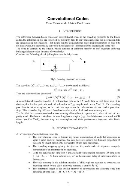
Consider the following circuit (all registers are initially zero):
u i
x i
Fig.1. Encoding circuit of rate ½ code
(1) (1)
(2) (2)
The code bits ( x , x , ) and ( x , x , ) are obtained as follows:
0 1
0 1
(1)
(2)
xi u i
and x
i
ui
ui
1
(1)
Then the codewords are generated:
(1) (2) (1) (2)
x (( x0 x0
),( x1
x1
), )
( x
0
, x1,
)
(2)
A convolutional encoder encodes K information bits to N > K code bits in each time step. It is
obvious, that for this particular code K 1 and N 2 , giving the code a rate R 1/ 2 . The encoding
procedure is not memoryless, as the code bits depend on the information bits encoded at past time
steps. This is another big difference from block codes, as the block codes are memoryless.
The fact that the convolutional codes have memory allows them to operate well, when K and N are
pretty small. The block codes have to have long block lengths (e.g., Reed-Solomon code used in CD
drives has N 2048 ), because they are memoryless and their performance improves with block
length.
II.
CONVOLUTIONAL CODES
A. Properties of convolutional codes [1]
The convolutional code is linear: any linear combination of code bit sequences is
again a valid code bit sequence. We can therefore specify the distance properties of
the code by investigating only the weights of non-zero sequences.
The encoding mapping u x is bijective, i.e., each code bit sequence uniquely
corresponds to an information bit sequence.
Code bits generated at time step i are affected by information bits up to M time steps
i 1,
i 2, i
M back in time, i.e., M is the maximal delay of information bits in
the encoder.
The code memory is the minimal number of shift registers required to construct an
encoding circuit for the code. The code memory is at most M K .
The constraint length is the overall number of information bits affecting code bits
generated at time step i : M K K ( M 1)
K
2

A convolutional code is systematic if the N code bits generated at time step i
contain the K information bits
Let us consider some examples:
(1)
x i
u i
x
i
(1)
u i
(2)
x i
(3)
x i
(2)
u i
Fig.2. This rate R 1/ 2 code has delay M 1,
memory 1, constraint length 2, and is systematic
Fig.3. This rate R 2 / 3 code has
delay M 1, memory 2, constraint length 4, and
is not systematic
B. Descriptions of convolutional codes
There are multiple ways to describe convolutional codes, the main are [1]:
Trellis
Matrix description
First, we consider the description using a trellis. Trellis is a directed graph with at most S nodes,
where S is the vector representing all the possible states of the shift registers at each time stepi . In all
the examples the rate R 1/ 2 code described in Fig.1. is used.
s
0
s1
s
0|00
0|00
2
0 0
0
0|01 1|11
1|11
1
1
1|10
We get the trellis section by considering the
operation of the encoding circuit:
M K
The trellis section has 2 nodes for each
time step.
It is obvious that s i
u i 1
, and the codeword
(1)
(2)
is obtained by x u and x u s .
i
The branches are labeled with u
i
| x
i
. So we
input a new information bit u and it is
written into the shift register, thus s
i
i
i
i
i1 i
,
i
u
and we get a codeword x
i
, generated with
this transition.
The trellis is growing exponentially with M .
As described in [1], we can define a convolutional code, using a generator matrix that describes the
encoding function u x :
x u G
(3)
where
3

G
0
G1
G
2
G
M
G
0
G1
G
2
G
M
G
G G G G
(4)
0 1 2
M
The ( K N)
submatricesG m
, m 0,1, ,
M , with elements from GF(2)
specify how an
information bit block u
i m
, delayed m time steps, affects the code bit block x
i
:
x
i
M
m0
u
im
G
m
, i
(5)
For this code (in Fig.1.) we need to specify two submatrices, G
0
and as the memory of this code
is M 1, also G
1
. The size of the submatrices must be ( K N)
, and as we have a rate R 1/ 2
code, both submatrices will be of size1 2 .
(1) (2)
The matrix G
0
governs how u
i
affects x
i
( xi
, xi
) : as u
i
affects the first bit of the codeword as
well as the second bit of the codeword the matrix G
0
= 1 1
.
The matrix G1
governs how u
i1
affects x
i
: as u
i1
affects only the second bit of the codeword but
not the first one the matrix G
1
= 0 1
.
For 3 information bit long sequence u u , u , ) using (3) we get
(
0 1
u2
(1) (2) (1) (2) (1) (2)
(( x0 x0
),( x1
x1
),( x2
x2
)) ( u0
, u1,
u2
) G
(6)
As we have 3 information bits at the input and we consider 3 time steps the generator matrix G must
be3 3. The generator matrix is obtained considering the operation of the encoding circuit:
u 0
At time t 0 we input u
0
, as there is
(1) (2)
( x x 0 0
) nothing in the register both code bits are
affected by u
0
. The generator matrix at this
time step is:
11
G
u 1
u 0
(1)
( x 1
x
(2)
1
)
At time t 1 we input u
1. As u0
is stored at
the register it affects only the second bit of
the code word, u1affects both bits of the
codeword. The generator matrix at this time
step is:
11
01
G 11
4

u 2
u 1
(1)
( x 2
x
(2)
2
)
At time t 2 we input u
2
. As u1is stored at
the register it affects only second bit of the
generated codeword, u2
affects both bits of
the codeword and u
0
doesn’t affect anything
as it was already deleted from the register.
Finally we obtain the whole generator
matrix:
11
01
G 11 01
11
C. Puncturing of convolutional codes
The idea of puncturing is to delete some bits in the code bit sequence according to a fixed rule. In
general the puncturing of a rate K / N code is defined using N puncturing vectors. Each table
contains p bits, where p is the puncturing period. If a bit is 1 then the corresponding code bit is not
deleted, if the bit is 0, the corresponding code bit is deleted. The N puncturing vectors are combined
in a N p puncturing matrix P .
Consider code in Fig.1. , without puncturing, the information bit sequence u (0,0,1,1,0 ) generates
the (unpunctured) code bit sequence x
NP
(00,00,11,01,01)
. The sequence x
NP
is punctured using a
puncturing matrix:
1
1 1 0
P 1
1
0 0 1
(1)
(2)
The puncturing period is 4. Using P 1
, 3 out of 4 code bits x
i
and 2 out of 4 code bits xi
of the
mother codes are used, the others are deleted. The rate of the punctured code is thus
R 1/
2 (4 4) /(3 2) 4 / 5 and u is encoded to x ( 00,0X
,1X
, X1,01)
= (00,0,1,1,01)
The performance of the punctured code is worse than the performance of the mother code. The
advantage of using puncturing is that all punctured codes can be decoded by a decoder that is able to
decode the mother code, so only one decoder is needed. Using different puncturing schemes one can
adapt to the channel, using the channel state information, send more redundancy, if the channel quality
is bad and send less redundancy/more information if the channel quality is better.
D. Decoding of convolutional codes
The very popular decoding algorithm for convolutional codes, used in GSM standard for instance, is
the Viterbi algorithm. It uses the Maximum likelihood decoding principle. The Viterbi algorithm
consists of the following steps for each time index [1]:
1. For all S state nodes at time step j, j 0,1, ,
L / N 1:
Compute the metrics for each path of the trellis ending in the state node. The metric
at the next state node is obtained by adding the path metric to the metric at the
previous corresponding state node. The path metric is obtained by the following
formula, : y x y
(7)
j
x1 j 1 j 2 j
2 j
where x is the sent bit, y is the received bit
If the two paths merge, choose the one with the largest metric, the other one is
discarded. If the metrics are equal, the survivor path is chosen by some fixed rule.
5

2. If the algorithm processed d trellis sections or more, choose the path with the largest metric,
go back through the trellis and output the code bit sequence and the information bit sequence.
The parameter d is the decision delay of the algorithm and specifies how many received
symbols have to be processed until the first block of decoded bits is available. As a rule of
thumb, the decision delay is often set to 5 M .
Let us consider a following encoding circuit:
x 1 j
u j
s 1 j
s 2 j
In Fig.4. the corresponding trellis is depicted:
x 2 j
+ 1 + 1
+ 1 / + 1 + 1
+ 1 + 1
- 1 / - 1 - 1
+ 1 - 1
+ 1 / + 1 - 1
+ 1 - 1
- 1 / - 1 + 1
- 1 + 1
- 1 / - 1 + 1
+ 1 / + 1 - 1
- 1 + 1
+ 1 / + 1 + 1
- 1 - 1
- 1 / - 1 - 1
- 1 - 1
s
1 j
, s
2 j
x
1 j
, x
2 j s
1 j 1
, s
2 j 1
Fig. 4. Trellis of convolutional code
The encoded sequence x ( 11,
11,
11,
11,
11,
11,
11)
(BPSK-modulated bits
considered). In the received sequence there are some errors introduced. Fig.5. and Fig.6. show that
hard-decision Viterbi algorithm is performing well in case of single errors.
+1+1
0
+1+1 -1+1 +1+1 +1+1 +1+1 +1+1 +1+1
+2
-2
+2
-2
0
0
-2
+2
+2
+2
-4
+2
-2
0
0
0
0
+4
0
+2
+2
0 -2 +2 0 +2 +4
+6
j=0 j=1 j=2 j=3 j=4 j=5 j=6 j=7
+1+1
0
û
j
+6
+2
+4
+8
+4
+2
+1 +1 +1 +1 +1 +1 +1 - No error
+10
Fig. 5. Performance of Viterbi algorithm in case of one single error
+1+1 -1+1 +1-1 +1+1 +1+1 +1+1 +1+1
+2
-2
+2
-2
0
0
-2
+2
+2
+2
-4
0
0
+2
+2 +2
-2
+2
+4
-2
+2
-2
0
0
0
0
+2
-2
0
0
0
0
+6
+4
+12
0 +2 +2 +2 +2
0 0 0 -2 +2 -2 +4 -2 +2 -2 +4
j=0 j=1 j=2 j=3 j=4 j=5 j=6 j=7
û
j
+4
+4
+2
+1 +1 +1 +1 +1 +1 +1 - No error
+6
+2
+4
+2
-2
0
0
0
0
+8
+4
+6
+2
-2
0
0
0
0
+8
+6
+10
+6
+4
6

Fig. 6. Performance of Viterbi algorithm in case of two single errors
Fig.7. shows that the performance of hard-decision Viterbi algorithm degrades significantly in case of
burst errors.
+1+1
0
+1+1 -1-1 -1+1 +1+1 +1+1 +1+1 +1+1
+2
-2
+2
-2
-2
+2
0
0
0
+4
-2
0
0
-2
+2
-2
+2
0
0
+2
+2
-2
0
0
0
0
+2
-2
0
0
0 +2 +2 +2 +2
-2 0 +6 -2 +4 -2 +2 -2 +8 -2 +6
j=0 j=1 j=2 j=3 j=4 j=5 j=6 j=7
û
j
+2
+2
+8
0
0
+8
+8
+6
+1 -1 -1 +1 +1 +1 +1 - 2 decoding errors
+2
-2
0
0
0
0
+10
Fig. 7. Performance of the Viterbi algorithm in case of error bursts
Fig.8. shows that the application of the soft-decisions Viterbi algorithm improves the situation as the
errors are corrected.
( m)
j
x1
jl1
j
y1
j
x2
jl2
j
y2
j
+6
+8
+2
-2
0
0
0
0
+12
+8
+10
l
j
- channel state information
l
j
2
0.5
“Good” channel
“Bad” channel
+1+1
0
+1+1 -1-1 -1+1 +1+1 +1+1 +1+1 +1+1
G B
+2.5
-2.5
+2.5
-2.5
B B
-1
+1.5
B G
+1.5
+3
G B
+2.5 +5.5
G G
+4
+9.5
G G
+4 +13.5
G G
2 0.5 0.5 0.5 0.5 2 2 0.5 2 2 2 2 2 2
+1
-1.5 -2.5 -4 -4 -4
+3.5 -2.5 0 +1.5 +0.5 +8.5
0 0 +7.5 0 +9.5
+2.5 -1.5 0 0 0
0
-2.5 +1.5 0 +7.5 0+8.5
0
-2.5 +1 +8.5
+12.5
0
+2.5 -1.5 0 0 0
+1.5 +2.5 +4 +4 +4
-2.5 -1.5 +6 -2.5 +3.5 +0.5 +8.5
-4 -4 -4 +7.5
+4
+17.5
j=0 j=1 j=2 j=3 j=4 j=5 j=6 j=7
Fig. 8. Performance of the soft-decision Viterbi algorithm in case of error bursts
III.
CONCLUSION
Convolutional codes are very easy to implement. Convolutional codes use smaller codewords in
comparison to block codes, achieving the same quality. Puncturing techniques can be easily applied to
convolutional codes. This allows generating a set of punctured codes out of one mother code. The
advantage is that to decode them all only one decoder is needed and adaptive coding scheme can be
thus implemented. One of the most important decoding algorithms is the Viterbi algorithm that uses
the principle of maximum likelihood decoding. The Viterbi decoding uses hard decisions is therefore
very vulnerable to error bursts. Using Soft instead of Hard decisions for Viterbi decoding improves the
performance.
REFERENCES
[1] M. Tuechler and J. Hagenauer. “Channel coding” lecture script, Munich University of
Technology, pp. 111-162, 2003
7