5.4 The Quadratic Formula - College of the Redwoods

More documents

Recommendations

Info

$Math 50A February 18, 2011 Quiz #10 Name: David Arnold ...$

$College of the Redwoods Math Lab What is the Math Lab course? The$

$Math Department Meeting Minutes April 19, 2013 in PS 117 3-â€5pm ...$

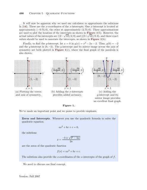
490 Chapter 5 Quadratic Functions It will now be apparent why we used our calculator to approximate the solutions in (14). These are the x-coordinates of the x-intercepts. One x-intercept is located at approximately (−0.73, 0), the other at approximately (2.73, 0). These approximations are used to plot the location of the intercepts as shown in Figure 1(b). However, the actual values of the intercepts are ((2− √ 12)/2, 0) and ((2+ √ 12)/2, 0), and these exact values should be used to annotate the intercepts, as shown in Figure 1(b). Finally, to find the y-intercept, let x = 0 in g(x) = x 2 − 2x − 2. Thus, g(0) = −2 and the y-intercept is (0, −2). The y-intercept and its mirror image across the axis of symmetry are both plotted in Figure 1(c), where the final graph of the parabola is also shown. y y y (1, −3) x ( √ ) ( √ ) 2− 12 2 , 0 2+ 12 2 , 0 x (1, −3) ( √ ) ( √ ) 2− 12 2 , 0 2+ 12 2 , 0 x (0, −2) (1, −3) x = 1 (a) Plotting the vertex and axis of symmetry. x = 1 (b) Adding the x-intercepts provides added accuracy. x = 1 (c) Adding the y-intercept and its mirror image provides an excellent final graph. Figure 1. We’ve made an important point and we pause to provide emphasis. Zeros and Intercepts. Whenever you use the quadratic formula to solve the quadratic equation the solutions are the zeros of the quadratic function ax 2 + bx + c = 0, x = −b ± √ b 2 − 4ac 2a f(x) = ax 2 + bx + c. The solutions also provide the x-coordinates of the x-intercepts of the graph of f. We need to discuss one final concept. Version: Fall 2007
Section 5.4 The Quadratic Formula 491 The Discriminant Consider again the quadratic equation ax 2 + bx + c = 0 and the solutions (zeros) provided by the quadratic formula x = −b ± √ b 2 − 4ac . 2a The expression under the radical, b 2 − 4ac, is called the discriminant, which we denote by the letter D. That is, the formula for the discriminant is given by D = b 2 − 4ac. The discriminant is used to determine the nature and number of solutions to the quadratic equation ax 2 +bx+c = 0. This is done without actually calculating the solutions. Let’s look at three key examples. ◮ Example 15. Consider the quadratic equation x 2 − 4x − 4 = 0. Calculate the discriminant and use it to determine the nature and number of the solutions. Compare x 2 − 4x − 4 = 0 with ax 2 + bx + c = 0 and note that a = 1, b = −4, and c = −4. The discriminant is given by the calculation D = b 2 − 4ac = (−4) 2 − 4(1)(−4) = 32. Note that the discriminant D is positive; i.e., D > 0. Consider the quadratic function f(x) = x 2 − 4x − 4, which can be written in vertex form f(x) = (x − 2) 2 − 8. This is a parabola that opens upward. It is shifted to the right 2 units, then downward 8 units. Therefore, it will cross the x-axis in two locations. Hence, one would expect that the quadratic formula would provide two real solutions (x-intercepts). Indeed, x = −(−4) ± √ (−4) 2 − 4(1)(−4) 2(1) = 4 ± √ 32 . 2 Note that the discriminant, D = 32 as calculated above, is the number under the square root. These solutions have approximations x = 4 − √ 32 2 ≈ −0.8284271247 and x = 4 + √ 32 2 ≈ 4.828427125, which aid in plotting an accurate graph of f(x) = (x − 2) 2 − 8, as shown in Figure 2. Version: Fall 2007
Page 1 and 2: Section 5.4 The Quadratic Formula 4
Page 9: Section 5.4 The Quadratic Formula 4
Page 15: Section 5.4 The Quadratic Formula 4

5.4 The Quadratic Formula - College of the Redwoods

Create successful ePaper yourself

Delete template?

Save as template?