RANS Study of Hydrogen-Air Turbulent Non-Premixed Flames

RANS Study of Hydrogen-Air Turbulent Non-Premixed Flames
D. Dovizio 1 , E. Giacomazzi 2 , C. Bruno 1 , A. Ingenito 1 , N. Arcidiacono 2
1. Univ. "Sapienza", Dept. Mechanics and Aeronautics , Rome - ITALY
2. ENEA, TER-ENE-IMP, Rome, ITALY
1. Test case description
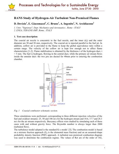
The coaxial air nozzle is concentric to the fuel nozzle, and the inner (d a ) and the outer
diameter are 30 and 38 mm, respectively. The coaxial air is injected parallel to the fuel jet. In
addition, coflow air is provided to the flame to keep the global equivalence ratio within a
certain range. The velocity of the coflow air is kept low enough not to affect flame
characteristics [1-2]. Flame stabilization is obtained by the thickness t of the hydrogen duct, t
= 5 mm. The fuel is hydrogen, flowing in the central duct, while the primary air stream flows
inside the annular duct: the two jets are ducted for 40mm prior to entering the combustion
chamber.
Fig. 1
Coaxial combustor schematic section.
Three simulations were performed, corresponding to three different injection velocities of the
fuel and oxidizer streams: 25, 50 and 106 m/s for the hydrogen stream and 10.6, 17.7 and 28.3
m/s for the air stream respectively. Buoyancy effects were studied by simulating each of these
cases with and without gravity force. The Reynolds number is always larger than 2000
(turbulent flow).
The turbulence model adopted is the standard K- model [3]. The combustion model is based
on a mixture fraction approach (Z H is the elemental mass fraction) and on an assumed-shape
probability density function (PDF) approach. A turbulent non premixed combustion diagram
was used to determine the combustion regime. The values of Ret are of the order of 102,
1

Processes and Technologies for a Sustainable Energy
while Da is of the order of 103: the laminar flamelet assumption (LFA) limit is justified for
the present study, offering tremendous computational savings.
2. Flame structure
In the flamelet approach the flame structure is described using the mixture fraction [4]. The
computed flame structure is plotted in Figure 2. This result underlines that in the flamelet
approach finite rate chemistry can be taken into account. Diffusion flame usually lies along
the points where mixing produces a stoichiometric mixture. Z H = Z st iso-surfaces give an idea
of the flame shape as shown in Figure 3.
Fig. 2
Temperature versus Z H plot defining flame structure (U H2 =106m/s with gravity).
Fig. 3
Stoichiometric mixture fraction iso-surface defining flame shape. 1 U H2 =25m/s with
gravity, 2 U H2 =25m/s without gravity; 3 U H2 =50m/s with gravity; 4 U H2 =50m/s
without gravity; 5 U H2 =106m/s with gravity; 6 U H2 =106m/s without gravity.
2

Ischia, June, 27-30 - 2010
Figure 3 shows results performed with URANS simulations for the three different injection
velocities configurations. For each of them gravity effect was considered by comparing
simulations with the gravity force included (on the left of each couple) and not (on the right).
These first results can be summarized with three mean features:
flame length increases when the inlet velocity increases,
gravity field makes the flame shorter,
but this effect is more evident for low injection velocities.
Physics interpretation of this behavior can be found recalling Froude number definition and
considering that increasing inlet velocity means increasing initial momentum flux with
respect to buoyant forces (i.e. Froude number): flame length (associated with the momentum
flux) increases. The second feature can be interpreted intuitively: gravity force acts opposing
to the flow motion and the flame is strongly affected due to the low hydrogen density value.
4. Temperature and velocity fields
Thermal field analysis, predicted by URANS simulations, show a well anchored flame with
the combustion initially limited to the thin shear layer where hydrogen and air mix. A cold
zone (blue depicted) can be identified, where only fuel exists and is generally called inertial or
potential core. Maximum temperature is reached on the axis, on a location increasing as
velocity injection increases. Buoyancy effects are evidenced by the presence of external
vortices at low axial locations. Fig. 6 shows instantaneous temperature fields comparing the
case with gravity force included with the one in absence of gravity.
Fig. 4
Instantaneous temperature fields for the three different cases: on the left is depicted
the case with .
5. Flame – vortex interaction
An instantaneous iso-temperature color visualization of the computed flame (U H2 = 106 m/s, no
gravity) is shown in Fig. 5a. It should be pointed out that no artificial perturbations were intro-
3

Processes and Technologies for a Sustainable Energy
duced to generate buoyancy-driven structures external to the flame. Once a vortex is developed it
rolls along the flame surface while it is convected downstream. During this process, the vortex
interacts strongly with the flame, making the flame surface bulge and squeeze. This motion is
simulated by the time-dependent calculations.
Fig. 5
Comparison of computed hydrogen/air flames for fuel-jet velocity of 106 m/s: (a)
instantaneous temperature contours of computed flame; (b) iso-temperature contours
obtained from time-averaged flame; (c) iso-temperature contours of steady-state
flame.
Since the mean temperature reflects the time the flame spends at a given location, the
presence of the first bulge indicates that the flame spends considerable time in the bulged
position at an axial location between 110 and 140 mm. The isotherms in the interior of the jet
(r < 5 mm) are only moderately affected by the dynamic motion of the outer structures, as
evidenced by the similarity of the instantaneous (Fig. 5a) and averaged (Fig. 5b) isotherms.
To illustrate the importance of simulating the dynamic flames using unsteady CFD codes,
calculations were also performed for the same flame using the steady-state option of
FLUENT. Solution for this case converged to a flame having perfectly smooth surface. The
iso-temperature visualization of the resulted flame is shown in Fig. 5c, which does not
resemble either the instantaneous flame (Fig. 5a) or time-averaged flame (Fig. 5b).
Fig. 6 Impact of outer and inner vortices on temperature for the flame shown in Fig. 5.
Blowups of the two different vortex-flame interactions are shown insets.
Vortex-flame interactions result in the presence of two types of vortices: one located on the
fuel side of the flame and the other on the air side. Both types of vortices create positive
(stretch) and negative (compression) stretch regions when interacting with the flame, as
4

Ischia, June, 27-30 - 2010
shown in Fig. 6. The outer vortex-flame interaction is shown in the left insert, and the fuel
side vortex-flame interaction is shown on the right. Vortices are more evident in the isoradial-velocities
contours of Fig. 7: red and blue colors represent positive (outward) and
negative (inward) radial velocities, respectively.
Fig. 7
Instantaneous radial velocity fields in the first part of the combustor for
: on the left is depicted the case with
Vortices motion are time dependent. Frequency spectra from the temperature fluctuations
(measured on a single point in the domain, x=10cm; y=0.95cm) are obtained using FFT
method. Figure 8 shows frequency spectra obtained from temperature data collected at a
radial location of 9.5 mm within the shear-layer at a distance of 100 mm from the nozzle exit.
The data, stored from 60000 time-steps, covered a real time of 0.6 s. We can distinguish two
peaks over a frequency range between 0 to 1000 Hz. The one at 273.9 Hz corresponds to the
fundamental frequency, and the subharmonic of this (547.8 Hz) appears as the second peak.
The frequency of the highest peak can be compared with a dimensional analysis that defines a
frequency as the ratio of mean velocity and characteristic length of the vortices:
(1)
where L v is the distance between two consecutive vortices. Vortex frequency value is very
close to the peak obtained from the FFT and displayed on Fig. 10. Physically this
phenomenon can be explained considering turbulent fluctuations as different spatial and
temporal scales vortical structure overlap. When these move inwards the fluid they induce a
perturbation on the characteristic scalars.
5

Processes and Technologies for a Sustainable Energy
Fig. 8
Frequency spectra obtained from temperature measured on a single point into the
domain ( ): , with gravity effects.
6. Conclusions
RANS and URANS simulations were performed for a turbulent jet diffusion flame. Buoyancy
effects were demonstrated by comparing temperature fields for cases with and without gravity
force included for different injection velocities. This analysis shows that buoyancy effects are
less evident for high injection velocities. Finally URANS simulations showed that in certain
cases transient phenomena such as flame vortex interactions can be predicted.
7. References
[1] J.F. Driscoll, R.H. Chen, and Y. Yoon: Combust. Flame 88:37-49, 1992.
[2] J.-Y. Chen and W. Kollmann: Combust. and flame 88, 1992.
[3] B.E. Launder and D.B. Spalding: Lectures in Mathematical Models of Turbulence.
London: academic Press., 1972.
[4] T. Poinsot and D. Veynante, Theoretical and numerical combustion, Edwards, 2005.
6