Calculating Iron Losses Taking into Account Effects ... - COMSOL.com

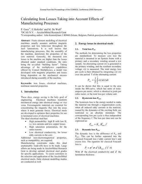
Excerpt from the Proceedings of the COMSOL Conference 2008 Hannover
Calculating Iron Losses Taking into Account Effects of
Manufacturing Processes
P. Goes *1 , E.Hoferlin 1 and M. De Wulf 1
1 OCAS N.V. – ArcelorMittal Research Gent
*Corresponding author: John Kennedylaan 3 B9060 Zelzate, Belgium, Patrick.goes@arcelormittal.com
Abstract: Finite element modelling of electrical
machines usually assumes uniform magnetic
properties and loss behaviour throughout the
steel laminations. It is well known that
manufacturing processes, like the assembly of
the machine, deteriorate the properties of the
core material. Generally, the measured iron
losses in the machine are higher than the losses
obtained under standard conditions, the ratio
being the so-called “building factor”. Taking
advantage of the multiphysics capabilities
offered by Comsol Multiphysics, a model was
developed with magnetic properties and losses
being dependent on the mechanical stresses
introduced during assembly of the machine.
Keywords: iron losses, electrical machines,
nonlinear material properties.
1. Introduction
These days, energy saving is the holy grail of
engineering. Electrical machines transform
mechanical energy into electrical energy or vice
versa. Ferromagnetic materials are essential for
concentrating the magnetic flux into the areas
where it must generate forces. Electrical steels
are developed to optimize their properties for use
in laminated cores of electrical machines.
The ideal electrical steel has:
• High permeability: high B with low H,
i.e. low currents and low copper losses.
• High saturation polarization, for the
same reasons.
• Low electrical conductivity, for lower
eddy currents in the core.
Additional non-electromagnetical properties,
such as stampability, are required.
Manufacturing constraints make this ideal
unattainable: trade-offs have to be made. Large
efforts are being made in ArcelorMittal Research
Gent to develop optimal electrical steel grades
for specific applications. To assist customers in
the selection and application of the ArcelorMittal
electrical steels, finite element modelling studies
are conducted as well.
2. Energy losses in electrical steels
2.1. Total loss P tot
The methods for determining the loss properties
are standardized. To measure core loss the
material is mounted in an Epstein frame with a
primary and a secondary winding around a test
sample. An alternating current i(t) is generated in
the primary winding, and the resultant secondary
voltage v(t) is measured. The total energy loss
per cycle is then obtained by integrating v(t) i(t)
over one period T of the alternating current:
P
tot
1
=
T
T
∫
0
v(
t)
i(
t)
dt
It can be shown that this is equal to the area
inside the BH-curve, which has units of teslaamperes
per meter, which is identical to joule per
cubic meter, or the total loss per volume unit.
2.2. Hysteresis loss P hyst
The hysteresis loss is the energy needed to make
the material run through a magnetization cycle,
when all induced eddy currents in the material,
caused by the dynamics of the exciting field, are
restricted to an absolute minimum. The
corresponding loss per cycle is thus independent
of the frequency f. The loss per time unit can be
expressed as:
P
hyst
= K
2.3. Dynamic loss P dyn
h
B
2
max
The dynamic loss is the difference of P tot and
P hyst . This can be further separated into the
classical Foucault loss (‘eddy current loss’) and
excess loss. The equation for classical Foucault
loss is:
P c
2 2
= π σ d ( B
max
f
f )
2
/ 6
With σ the electrical conductivity and d the
lamination thickness

3. Effect of mechanical stresses on the
magnetic properties
The dependence of magnetic properties on
mechanical stress during elastic and plastic
deformation can be evaluated by means of
special constructed equipment, ([Permiakov
2002]) consisting of a single sheet tester in
which unidirectional tensile and compressive
loads can be applied to the specimen.
3.1. Effect on the magnetization loop
In general, the shape of the magnetization loops
is changing during the application of stress, see
Figure 1. The coercive field is increasing while
the remanent induction and the permeability are
decreasing.
Figure 2. Variation of hysteresis loss as a
function of mechanical stress.
4. Application in the modelling of
electrical machines
Figure 1. Variation of magnetization loops under
mechanical stress.
Effect on the hysteresis losses
Figure 2 depicts the hysteresis losses as a
function of the tensile stress for the
magnetization levels of 0.7, 1.0 and 1.2 Tesla
and 50Hz sinusoidal magnetic flux.
The stator of electrical machines is often
assembled with the housing by means of pressor
interference fitting. The housing inner
diameter is slightly smaller than the stator’s
outer diameter. The housing can then be
mounted by heating it, sliding it over the stator,
and allowing it to cool. The shrinking housing
compresses the stator core, and, as mentioned in
the preceding paragraph, these mechanical
stresses deteriorate the magnetic properties of the
electrical steel.
We developed a model in Comsol multiphysics
to quantify these effects.
5. Solving for the interference fitting
stresses
The stresses occurring in the stator were
calculated using the plane strain (smpn)
application mode of the structural mechanics
module, by including a thermal expansion load
on the housing’s subdomain and letting it cool
down from a reference strain temperature down
to the ambient strain temperature.

2
1.5
s=0MPa
s=20MPa
s=40MPa
B[T]
1
0.5
Figure 3. von mises stress field
0
0 500 1000 1500
H[A/m]
Figure 4. B-H curve as function of stress
2
1.5
B[T]
1
0.5
Figure 4. von mises stress along a radius
The line plot shows compressive stresses inside
the stator and tensile stresses in the housing, as
expected.
This stress state is subsequently used to modify
the magnetic properties of the stator material.
6. Modelling the magnetic properties
For simulation purposes, the magnetization
curve of electrical steel can be expressed as a
function of just two parameters: the saturation
polarization Js and the relative permeability µ r :
2 J
s
π ( µ
r
−1)
µ
0
H
B( H ) = µ
0
H + arctg
π
2 J
s
The effect of the stress can be introduced by a
correction factor:
B H S B H K B
( , ) = ( ,0) (1 + S)
With the factor KS = 0.0035 determined by
fitting to experimental data, stresses being
expressed in MPa.
S
0
0
-20
S[MPa]
-40
-60
0
200
400
H[A/m]
As the emqa equation system needs H as a
function of B, the above function has to be
inversed.
H[A/m]
10000
8000
6000
4000
2000
0
0
-20
S[MPa]
-40
-60
0
This H(B,S) function is implemented in the
Comsol model as a 2D interpolated table-lookup
function.
7. Solving for the magnetic flux density
2D models of electrical machines are well suited
for the perpendicular induction currents, vector
potential (emqa) application mode: the currents
are perpendicular to the modelling plane. This
0.5
B[T]
1
600
1.5
800
1000
2

implies that the magnetic field is present only in
the modelling plane. Hence the magnetic vector
potential has only one nonzero component,
perpendicular to the modelling plane. Maxwell’s
equations simplify to a second-order scalar PDE
with this magnetic potential component Az as
dependent variable.
The constitutive relation to be used is
H = f(|B|).e B , with e B the unit vector pointing in
the direction of the B-field.
The AC/DC module’s application mode supports
nonlinear relationships between H and B.
Here however, we need H = f(|B|,S).e B , and this
requires some modification of the equation
system:
By default, the expressions for Hx_emqa and
Hy_emqa refer to the HB interpolation function
of the chosen material, e.g. mat1_HB:
if(normB_emqa==0,nojac(pdiff(mat1_HB(norm
B_emqa[1/T])[A/m],normB_emqa))*Bx_emqa,ma
t1_HB(normB_emqa[1/T])[A/m]*Bx_emqa/normB
_emqa)
These expressions have to be modified in order
to refer to the 2D interpolation function that
describes the H = f(B,S), e.g. myHB2D:
if(normB_emqa==0,nojac(pdiff(myHB2D(normB
_emqa[1/T],mises_smpn[1/Pa])[A/m],normB_e
mqa))*Bx_emqa,myHB2D(normB_emqa[1/T],mise
s_smpn[1/Pa])[A/m]*Bx_emqa/normB_emqa)
By first solving the smpn-physics for the stress
and subsequently solving emqa, one finds the B-
field degraded by the effects of the mechanical
stresses.
8. Postprocessing for the losses
It is then a very simple matter to define the
above expressions for the loss components as
subdomain expressions, to generate loss maps,
and to integrate over complete cycles of the
machine to determine the overall core loss.
9. Electrical steels material library
A material library was developed, containing the
ArcelorMittal electrical steels properties.
10. Table 1: variables defined for electrical steels
variable Font Description
Js 2.1 [T] Saturation
magnetic
polarization
mur0 8000 Relative
permeability at
H=0
Kh 420
[W*s*T^-
3*m^-3]
Hysteresis loss
coefficient
Ke 0.96 Excess loss
coefficient
d 0.2[mm] Lamination
thickness
sigma 3.2e6[S/m] Electric
conductivity
11. Conclusions
Performing these calculations using typical
electromagnetic FEA products requires splitting
the geometry into discrete affected and nonaffected
zones and assigning different material
properties to each zone. As shown here, Comsol
allows for continuous adaptation of the magnetic
material properties, based on previous geometric
and/or structural mechanical results.
12. References
1. G.Bertotti, General properties of power losses
in soft ferromagnetic materials, IEEE Trans. On
Magn., 24, p.621-630 (1988)
2. V.Permiakov, A.Pulnikov, L.Dupré, M.De
Wulf, J.Melkebeek, Magnetic properties of Fe-Si
steel depending on compressive and tensile
stresses under sinusoidal and distorted
excitations, J.Appl.Phys., 93, p.6689-6691
(2003)