J_src_jrg_box_coeff_..

Box Coefficients
Sediment Records Computation
USGS National Training Center
May 2010
John R. Gray
USGS Office of Surface Water
jrgray@usgs.gov

What is a “Box Coefficient?”
It‟s USGS Jargon…
• A mean flow-weighted x-sectional
constituent concentration divided by a
mean concentration at a point or vertical.
Mean Concentration x-section mg/L
-----------------------------------------
Mean Concentration partial mg/L

Coefficient Derivation Example
• Pumped sample conc:
74, 67, 77, 79 mg/L
– Mean value is 74.25 mg/L
• X-section conc:
90 and 98 mg/L
– Mean value is 94.0 mg/L
• Box Coefficient = 94.0/74.3 = 1.27
• If this coefficient proved to be constant over time and
range of discharges – don’t count on it – one would
multiply all concentrations from pumped samples by
1.27 to obtain mean x-section sed conc.

Importance of the Box Coefficient
• After data density -- missing record -- the
derivation and application of the box
coefficient is the most important variable
in computation of daily sediment records.
• The box coefficient serves as a guide for
locating, or relocating, the sampling
vertical or sampler intake.

Some Factors in the Spatial
Distribution of Sediment
• Stokes Law (~size distribution of sediment)
• Proximity to upstream tributaries
• Bedforms, or lack thereof
• Channel alignment and secondary motion
• Bank stability
• Local features (natural and human-made)
• Source and type of sediment
• Discharge
• Season (indirect variable)
• Location of sampling location/intake with respect
to on-stream features and range-of-stage

Box Coefficient (BC) = C mean /C point
C mean = ~930 mg/l
BC=~1.1
BC=~1.1
BC=1.03
BC=~1

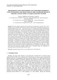
Box Coefficient (BC) = C mean /C point
C mean = ~1,360 mg/l
BC=~4
BC=~5
BC=~1.7
BC=~1.5

Incomplete mixing,
downgradient from
Bering Glacier,
SE Alaska

Colorado
River
.
Cisco
Drains 1/8
Of the
Lower 48
USA
Land Area

Double-Mass
Curve for
Green River at
Flaming Gorge
Dam Completed
November 1962
Green River, Utah
1930-82
X-axis: cumulative annual
water discharges
Y-axis: cumulative annual
suspended-sediment
load
~1945
(from Thompson, 1984)

Double-Mass
Curve for
Blue Mesa Reservoir Dam
Closed November 1965
Colorado River
at Cisco, Utah
1930-82
X-axis: cumulative
annual water
discharges
Y-axis: cumulative
annual suspendedsediment
load
(from Thompson, 1985)
~1945

Double-Mass
Curve for
San Juan River
Record Daily Sediment
Load, October 20, 1972
near Bluff,
Utah
1930-80
X-axis: cumulative
annual water
discharges
Y-axis: cumulative
annual suspendedsediment
load
~1944
(from Thompson, 1982)

Hypothesized Causative
http://water.
Factors: Changes in…
• Land-Use?
• Vegetation?
• Climate?
• Intrinsic Tributary Geomorphic
Processes?
• Or… (Topping et al, 1996)

The Colorado
River Sampler
Used until the
mid-1940’s

The US-D43 Isokinetic Suspended-Sediment Sampler.
Isokinetic samplers used by Fed. Gov’t since mid-1940’s

Site Selection, Not At Existing Gage
(subtitled, “Before the damage is done?”)
• Section or reach that has high
potential for being “typical” for
constituent to be measured over a
broad range of flows (bedload vs
suspended load).
• MUST be in sync with project
objectives and target data base.

Site Selection, Not At Existing Gage
(subtitled, “Before the damage is done?”)
• Some Desirable Characteristics:
- No untractable safety issues over range
of manual measurements (a must)
- Stable stage-discharge relation
- Accessible and measurable at all flows
- Ability to measure all flows at same
section
- No artifacts attributable to local
in-stream features

Site Selection, Not at Existing Gage
(continued)
• Measure at range of flows – particularly
medium and high flows – minimum
~8-section EDI measurements before
installing fixed sampling equipment.
• Install fixed sampling equipment based on
information derived from above efforts.
Goal is to obtain box coefficients nearest to
1.0 over range of flows, but particularly at
medium-to-high flows (important concept!)

Utilizing an Existing Gage
(subtitled, “After the damage is done?”)
• If unrushed (yes, I do have a sense of humor), use
methods described in previous slides for “new site.”
• More typically, must install equipment and start
monitoring immediately; in that case:
- Use best judgment for installing fixed
sampling features.
- Consider using “Gray‟s „1/3‟ rule-of-thumb”
(select vertical 1/3 from either side of stream –
why? Middle & edges are ~atypical sections)
- Use EDI method. Try to have one section
coincide with the fixed sampling point.

Some Tips for Minimizing Problems
• SOP: Scrutinize samples upon collection.
- Is there a visual correlation between
estimated concentrations in samples
(adjusting for water volume)?
- Do x-section to box sample estimated
concentrations compare favorably?
- Is there a reason to anticipate problems in
the record-computation step? If “yes”
remain at site/take additional samples…

Some Tips for Minimizing Problems
(continued)
• Take good notes intended for anyone‟s use
(think 2 decades hence – will your notes
be understandable and relevant?)
• Have EDI samples analyzed separately;
display on a cross-sectional plot. At least
one full particle-size analysis/sand-fine split.
• Use particle-size distributions to identify
trends and problems.
• Data collector should be record worker.

Box Coefficient Analysis Steps
Primary Data Review
• Job #1: Separate the Data from the Doodoo.
- Are data consistent with other evidence?
Good indicator if not necessarily “good”
- If inconsistent, not necessarily bad.
- Can you discredit data based on lab info,
field notes, sedimentological theory,
other information? If so, clearly
document rationale, outcome.

Box Coefficient Analysis Steps
(Primary Data Review, cont.)
• Try to discredit data that plot oddly; if you are
unsuccessful, ask yourself:
- Do you know more than what the sample
is “telling you”?
- How influential is the sample (flow rate, etc)?
- How often are you dealing with such
problems, and how to minimize them?
Relation between lab work and field work key.

Box Coefficient Analysis Steps
(Primary Data Review, cont.)
• Adulterated samples almost always result
in larger concentration values.
• Be reluctant to discard data points.
• Be ***extremely*** reluctant to discard
hydrographer x-sections. If results aren’t
used, why bother to collect these data?
• Document, document, document.

Box Coefficient Analysis Steps
(Primary Data Review, Example.)
• EDI cross-section sample values:
55, 50, 66, 58, 596; mean = 165 mg/L
• Observer box values:
57, 65, 66, 64, 63; mean = 63 mg/L
• Dude, what do I do?!?!
(a) panic -- suffer your 19 th nervous breakdown
(b) punt
(c) call John…

Box Coefficient Analysis Steps
(Primary Data Review, Example.)
Outlier included:
Conc mean = 165 mg/L
Box Coefficient = 2.62
Outlier excluded:
Conc mean = 63 mg/L
Box Coefficient = 1.10
700
700
600
Concentration, mg/L
600
500
EDI X-Section from Left Bank
500
400
400
300
300
200
200
100
100
0
1 2 3 4 5
0
1 2 3 4 5

Box Coefficient Analysis Steps
Trend Analysis
• Discharge Trends: Most common, have
physical basis, hydrographer’s 1st choice.
• Time Trends: Laborious to apply
correctly; objective rarely achieved.
• Concentration Trends: Sometimes
informative, but no slick method to apply.
• Phase of the Moon…?

Box Coefficient Analysis Steps
Magnitude of Box Coefficients
• No hard-and-fast, nor statistically based
rules -- yet; site and data dependent.
• Rule of thumb: 0.67 to 1.5 “tractable.”
• Unusually small (~2)
coefficients are often cause for concern;
influence of computational process
becomes inordinately large –
“manhandling the data”

Box Coefficient Analysis Steps
Magnitude, Box Coefficients (cont.)
• Where no trends are evident, data are
more or less evenly distributed around a
constant (ideally 1.0), may use constant.
• Where trends are evident, varying
coefficients should always be applied.

Box Coefficient Analysis Steps
Magnitude, Box Coefficients (cont.)
• Streams carrying smaller sediment
concentrations, and/or streams with
comparatively large amounts of sand, tend to
have widely varying coefficients.
• Hellacious or widely varying coefficients are a
signal to change something: The location of
the fixed sampling equipment, QC practices,
etc. Before changes, ask, “will it help?”

Box Coefficient Analysis Steps
Magnitude, Box Coefficients (cont.)
• Insufficient data and coefficients of 1.0:
- Should 1.0 coefficient be the default?
- Is there a physical basis for this?
- Are 1.0 coefficients just convenient?
- Is a coefficient of 1.0 equivalent to:
1.0000? 0.99-1.01? 0.9-1.1? 1.25-0.8?

Box Coefficient Analysis Steps
Application
• GCLAS – a brave new world…
- Capability to apply discharge, time, and
discharge+time-weighted coefficients.
- Good news – better, faster data
computations, easier verification.
- Bad news…You now have No Excuses
in credible application of coefficients!

Box Coefficient Analysis Steps
Advice
• Don’t sweat low-flow coefficients.
- Low-concentration (

Box Coefficient Analysis Steps
Advice (cont.)
• Try to identify coefficient-discharge
relations and apply by methods analogous
to stage-shift variation for discharge.
• Sample at-a-point sequentially to develop
a time series that sheds light on variance
on in-stream processes
• Automatic samplers need extra attention.

Box Coefficient Analysis Steps
Advice (cont.)
• Beware of comparing results from data
collected in different sections (Des Plaines
River at Riverside example).
• Avoid data collection in eddies.
• NO cross-sectional data collected???!!!
- Obvious first question…why not?
- Ask: What is data quality? Answer?
- May need to consider another approach –
surrogate technology?

Box Coefficient
Yellow Creek near Middlesboro, KY,
3.50
3.00
2.50
2.00
1.50
1.00
0.50
0.00
WY 1992
6/11 9/19 12/28 4/6 7/15 10/23
Date

Box Coefficient
Yellow Creek near Middlesboro, KY,
WY1992
3.50
3.00
2.50
2.00
1.50
1.00
0.50
0.00
0 1000 2000 3000 4000 5000
Discharge

Box Coefficient
Yellow Creek near Middlesboro, KY,
WY1992
3.50
3.00
2.50
2.00
1.50
1.00
0.50
0.00
0 1 2 3 4
Log10 Discharge, cfs

Box Coefficient
Cumberland River at Williamsburg, KY
2.00
1.50
1.00
0.50
0.00
11-Jun-
91
19-Sep-
91
28-Dec-
91
06-Apr-
92
15-Jul-
92
23-Oct-
92
Date

Box Coefficient
Cumberland River at Williamsburg, KY
2.00
1.50
1/10/92
1.00
0.50
0.00
0 1000 2000 3000 4000
Discharge, cfs

Box Coefficient
2.00
1.75
1.50
1.25
1.00
0.75
0.50
0.25
0.00
Cumberland River at Williamsburg, KY
(additional data from other years)
1/10/92
0 10000 20000 30000 40000
Discharge, cfs

Box Coefficient
Green River at Mumfordville, KY
12
10 11
9
8
7
6
5
4
3
2
0 1
09/19/91 12/28/91 04/06/92 07/15/92 10/23/92
Date

Box Coefficient
Green River at Mumfordville, KY,
WY1992
10 11 9
8
7
6
5
4
3
2
0 1 0 2000 4000 6000
Discharge, cfs

Box Coefficient
Green River at Mumfordville, KY
Coefficient = 10.77 Removed
3.00
2.50
2.00
1.50
1.00
0.50
0.00
0 2000 4000 6000
Discharge, cfs

Box Coefficient
Rio Puerco near Bernardo, NM
2.50
2.00
1.50
1.00
0.50
0.00
7/24/98 11/1/98 2/9/99 5/20/99 8/28/99 12/6/99

Box Coefficient
Rio Puerco near Bernardo, NM
2.50
2.00
1.50
1.00
0.50
0.00
0 50 100 150 200 250 300 350
Discharge, cfs

Box Coefficient
San Joaquin River near Vernalis, CA
1.400
1.200
1.000
0.800
0.600
0.400
0.200
0.000
7/24/98 11/1/98 2/9/99 5/20/99 8/28/99 12/6/99

Box Coefficient
San Joaquin River near Vernalis, CA
1.400
1.200
1.000
0.800
0.600
0.400
0.200
0.000
0 2000 4000 6000 8000 10000 12000 14000
Discharge, cfs

Hellbranch Creek, Ohio, WY 97

Box
Coefficient
6
5
4
3
2
1
0
Elwha River above Lake Mills,
Port Angeles, WA (1 of 2)
(approximate, from old graph sheets)
9/8/95 12/17/95 3/26/96 7/4/96 10/12/96
Date

Box Coefficient
Elwha River above Lake Mills,
Port Angeles, WA (2 of 2)
6
5
4
3
2
1
0
0 2000 4000 6000 8000
Discharge, cfs

ISCO coefficient ratio
iisco coeff ratio
0.400
Alameda Creek below Welch Creek near Sunol,
CA
0.350
0.300
0.250
0.200
0.150
Series1
Linear (Series1)
0.100
0.050
0.000
9/25/2007 11/14/2007 1/3/2008 2/22/2008 4/12/2008 6/1/2008
time
Alameda Creek below Welch Creek near Sunol
1.000
0.900
0.800
0.700
0.600
0.500
0.400
`
0.300
0.200
0.100
0.000
0.00 20.00 40.00 60.00 80.00 100.00 120.00 140.00
Discharge, in cfs

Box Coefficient Ratio
Box Coefficient Ratio
2.00
Sacramento River at Freeport, CA
1.80
1.60
1.40
1.20
1.00
box_vs_time
0.80
0.60
0.40
0.20
0.00
9/1/2002 1/14/2004 5/28/2005Time
10/10/2006 2/22/2008 7/6/2009
Sacramento River at Freeport, CA
2.00
1.80
1.60
1.40
1.20
1.00
0.80
0.60
0.40
0.20
0.00
0 10000 20000 30000 40000 50000 60000 70000 80000 90000 100000
Discharge, in cfs