Least Squares Temporal Difference Actor-Critic Methods with ...

where ψ θ (x, u) = 0 when x, u are such that µ θ (u|x) ≡
0 for all θ. It is assumed that ψ θ (x, u) is bounded
and continuously differentiable. Note that ψ θ (x, u) =
(ψθ 1(x, u), . . . , ψn θ
(x, u)) where n is the dimensionality of θ.
The convergence of the algorithm is stated in the following
Theorem (see the technical report [18] for the proof).
Theorem III.1 [Actor Convergence] For the LSTD actorcritic
with some step-size sequence {β k } satisfying (7), for
any ɛ > 0, there exists some λ sufficiently close to 1, such
that lim inf k ||∇ᾱ(θ k )|| < ɛ w.p.1. That is, θ k visits an
arbitrary neighborhood of a stationary point infinitely often.
IV. THE MRP AND ITS CONVERSION INTO AN SSP
PROBLEM
In the MRP problem, we assume that there is a set of
unsafe states which are set to be absorbing on the MDP
(i.e., there is only one control at each state, corresponding to
a self-transition with probability 1). Let X G and X U denote
the set of goal states and unsafe states, respectively. A safe
state is a state that is not unsafe. It is assumed that if the
system is at a safe state, then there is at least one sequence of
actions that can reach one of the states in X G with positive
probability. Note that this implies that Assumption A holds.
In the MRP, the goal is to find the optimal policy that
maximizes the probability of reaching a state in X G from
a given initial state. Note that since the unsafe states are
absorbing, to satisfy this specification the system must not
visit the unsafe states.
We now convert the MRP problem into an SSP problem,
which requires us to change the original MDP (now denoted
as MDP M ) into a SSP MDP (denoted as MDP S ). Note that
[3] established the equivalence between an MRP problem and
an SSP problem where the expected reward is maximized.
Here we present a different transformation where an MRP
problem is converted to a more standard SSP problem where
the expected cost is minimized.
To begin, we denote the state space of MDP M by X M , and
define X S , the state space of MDP S , to be
X S = (X M \ X G ) ∪ {x ∗ },
where x ∗ denotes a special termination state. Let x 0 denote
the initial state, and U denote the action space of MDP M .
We define the action space of MDP S to be U, i.e., the same
as for MDP M .
Let p M (j|x, u) denote the probability of transition to state
j ∈ X M if action u is taken at state x ∈ X M . We now define
the transition probability p S (j|x, u) for all states x, j ∈ X S
as:
⎧
⎨
p S (j|x, u) =
⎩
∑
i∈X G
p M (i|x, u), if j = x ∗ ,
p M (j|x, u), if j ∈ X M \ X G ,
for all x ∈ X M \ (X G ∪ X U ) and all u ∈ U. Furthermore, we
set p S (x ∗ |x ∗ , u) = 1 and p S (x 0 |x, u) = 1 if x ∈ X U , for all
u ∈ U. The transition probability of MDP S is defined to be
the same as for MDP M , except that the probability of visiting
(9)
the goal states in MDP M is changed into the probability of
visiting the termination state; and the unsafe states transit to
the initial state with probability 1.
For all x ∈ X S , we define the cost g(x, u) = 1 if x ∈ X U ,
and g(x, u) = 0 otherwise. Define the expected total cost
of a policy µ to be ᾱµ S = lim t→∞ E{ ∑ t−1
k=0 g(x k, u k )|x 0 }
where actions u k are obtained according to policy µ in
MDP S . Moreover, for each policy µ on MDP S , we can
define a policy on MDP M to be the same as µ for all states
x ∈ X M \ (X G ∪ X U ). Since actions are irrelevant at the goal
and unsafe states in both MDPs, with slight abuse of notation
we denote both policies to be µ. Finally, we define the
Reachability Probability Rµ
M as the probability of reaching
one of the goal states from x 0 under policy µ on MDP M .
The Lemma below relates Rµ M and ᾱµ:
S
Lemma IV.1 For any RSP µ, we have R M µ = 1
ᾱ S µ +1.
Proof: See [18].
The above lemma means that µ as a solution to the SSP
problem on MDP S (minimizing ᾱ S µ) corresponds to a solution
for the MRP problem on MDP M (maximizing R M µ ). Note that
the algorithm uses a sequence of simulated trajectories, each
of which starting at x 0 and ending as soon as x ∗ is visited for
the first time in the sequence. Once a trajectory is completed,
the state of the system is reset to the initial state x 0 and the
process is repeated. Thus, the actor-critic algorithm is applied
to a modified version of the MDP S where transition to a goal
state is always followed by a transition to the initial state.
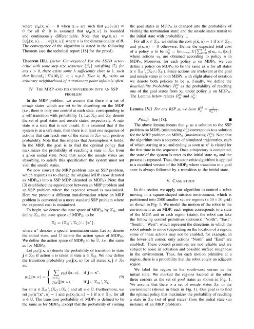
V. CASE STUDY
In this section we apply our algorithm to control a robot
moving in a square-shaped mission environment, which is
partitioned into 2500 smaller square regions (a 50 × 50 grid)
as shown in Fig. 1. We model the motion of the robot in the
environment as an MDP: each region corresponds to a state
of the MDP, and in each region (state), the robot can take
the following control primitives (actions): “North”, “East”,
“South”, “West”, which represent the directions in which the
robot intends to move (depending on the location of a region,
some of these actions may not be enabled, for example, in
the lower-left corner, only actions “North” and “East” are
enabled). These control primitives are not reliable and are
subject to noise in actuation and possible surface roughness
in the environment. Thus, for each motion primitive at a
region, there is a probability that the robot enters an adjacent
region.
We label the region in the south-west corner as the
initial state. We marked the regions located at the other
three corners as the set of goal states as shown in Fig. 1.
We assume that there is a set of unsafe states X U in the
environment (shown in black in Fig. 1). Our goal is to find
the optimal policy that maximizes the probability of reaching
a state in X G (set of goal states) from the initial state (an
instance of an MRP problem).