Download full text - ELSA - Europa

European Laboratory for 

Structural Assessment 

Proceedings of a Course on 

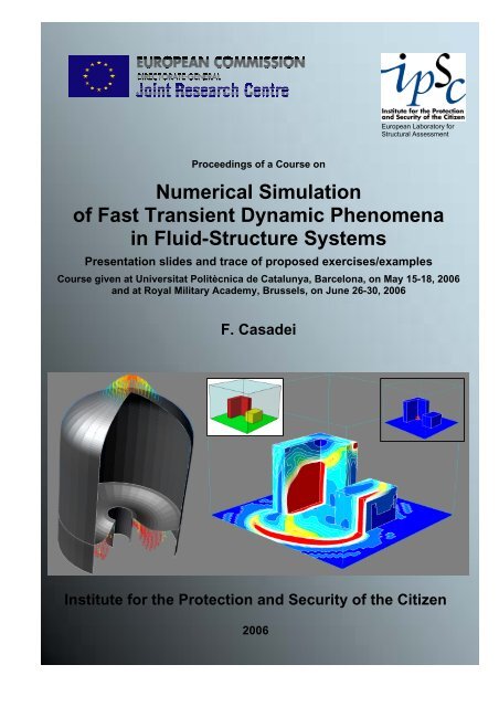
Numerical Simulation 

of Fast Transient Dynamic Phenomena 

in Fluid-Structure Systems 

Presentation slides and trace of proposed exercises/examples 

Course given at Universitat Politècnica de Catalunya, Barcelona, on May 15-18, 2006 

and at Royal Military Academy, Brussels, on June 26-30, 2006 

F. Casadei 

Institute for the Protection and Security of the Citizen 

2006

The mission of the Institute for the Protection and Security of the Citizen is to provids research- based, systemsoriented 

support to EU policies so as to protect the citizen against economic and technological risk. The Institute 

maintains and develops its expertise and networks in information, communication, space and engineering 

technologies in support of its mission. The strong cross-fertilisation between its nuclear and non-nuclear activities 

strengthens the expertise it can bring to the benefit of customers in both domains. 

European Commission 

Directorate-General Joint Research Centre 

Institute the Protection and Security of the Citizen 

Contact information 

Address: Folco Casadei 

E-mail: folco.casadei@jrc.it 

Telephone : +39 033278 9563 

Fax : +39 033278 9049 

http://ipsc.jrc.ec.europa.eu/home.php 

http://www.jrc.cec.eu.int 

Legal Notice 

Neither the European Commission nor any person acting on behalf of the 

Commission is responsible for the use which might be made of this publication. 

A great deal of additional information on the European Union is available on the Internet. 

It can be accessed through the Europa server 

http://europa.eu.int 

© European Communities, 2006 

Reproduction is authorised provided the source is acknowledged 

Printed in Italy

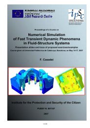
Proceedings of a Course on: 


of Fast Transient Dynamic Phenomena 


(Presentation slides and trace of proposed exercises/examples) 

A Short Course given by: 

F. Casadei 

at 

Universitat Politècnica de Catalunya, Barcelona, 15-18 May 2006 

and 

Royal Military Academy, Brussels, 26-30 June 2006

The present document contains the presentation slides and the traces of 

proposed exercises/examples related to the Course: Numerical Simulation 

of Fast Transient Dynamic Phenomena in Fluid-Structure Systems, 

given by F. Casadei at the Universitat Politècnica de Catalunya, Barcelona, 

15-18 May 2006 and at the Royal Military Academy, Brussels, 26- 

30 June 2006. 

This is the third, competely revised edition of the document: 

(1st Edition): “Proceedings of a Course on: Numerical Simulation of Fast Transient Dynamic Phenomena 

in Fluid-Structure Systems, Presentation Slides and Trace of Proposed Exercises/Examples, JRC — 

Ispra, 11-15 April 2005”, JRC Special Publication N. S.P.I.05.93, 2005. 

(2nd Edition): “Proceedings of a Course on “Numerical Simulation of Fast Transient Dynamic Phenomena 

in Fluid-Structure Systems. Presentation slides and trace of proposed exercises/examples”, Course 

given at Universitat Politècnica de Catalunya, Barcelona, on May 17-20, 2005, JRC Special Publication 

N. I.05.139, June 2005 

Numerous corrections and ameliorations have been carried out in the presentation slides and a number 

of new proposed practical exercises and examples have been added. Furthermore, Part 4 (Advanced topics 

and applications) has been enriched by a new topic, Spatial time step partitioning.

Programme of the Course 

1. Introduction 

a. Introductory example of a FSI problem 

i.Application spectrum and goals 

b. Modeling the structural domain 

i.Equilibrium equations 

ii.Explicit time integration scheme 

c. Treatment of essential boundary conditions 

i.The Lagrange multipliers method 

ii.Solving the linear system 

2. ALE formulation 

a. Modeling the fluid domain 

i.Euler equations 

ii.Finite Element discretization 

iii.Finite Volume discretization 

b. Mesh rezoning algorithms 

i.Motivation 

ii.Mean-based algorithms 

iii.Giuliani’s algorithm 

c. Free surface modeling 

3. ALE Fluid-Structure Interaction 

a. Motivation 

b. Classification of FSI algorithms 

c. Equilibrium-based methods 

i.The Uniform Pressure (UP) method 

ii.Shortcomings 

d. Geometrical methods 

i.The FSA/FSR method 

ii.Shortcomings 

e. A combined method 

i.The FSCR method 

4. Advanced topics and applications 

a. ALE description of structures 

b. Non-conforming FSI 

c. Lagrangian contact 

i.Classical methods 

ii.Pinballs 

iii.SPH 

d. Spectral elements 

e. Spatial time step partitioning 

f. Domain decomposition



of Fast Transient Phenomena 


A Short Course by F. Casadei 

European Commission, Joint Research Centre 


T.P. 480, I-21020 Ispra (VA), Italy. 

E-mail: Folco.Casadei@jrc.it 

1 

Contents 

• Introduction 

• ALE formulation 

• ALE Fluid-Structure Interaction 

• Advanced topics and applications 

2 

1

Credits & Acknowledgments 

• Structural Dynamics team at JRC Ispra (70’s – to date): 

– J. Donea, J.P. Halleux, S. Giuliani, … 

• Structural Dynamics team at CEA Saclay (70’s – to date): 

– H. Bung, P. Galon, M. Lepareux, … 

• Contributions from research/academic bodies and industry: 

– Barcelona (A. Huerta), Cachan, CRS4, Lyon, … 

– EDF, ENEL, Snecma, … 

• Three decades of code develompent: 

– EURDYN, Castem-PLEXUS / PLEXIS-3C, EUROPLEXUS … 

– Commercial version now available from SAMTECH S.A. 

3 

Introductory Example (Courtesy of ENEL-Hydro) 

4 

2

Introductory Example (2) 

5 


6 

3


7 

Application Spectrum 

• Energy (safety issues): nuclear and fossil-fueled plants, 

electrical devices, chemical plants, pressure vessels, … 

• Civil engineering: earthquakes, soil-structure interactions, 

attacks … 

• Marine/Offshore: ships and submarines, oil industry, 

pipelines, cables … 

• Transportation: crash, road barriers, tunnels safety, … 

•etc… 

8 

4

Goals/Characteristics 

• Simulate fast transient dynamic phenomena: 

explosions, crashes, impacts … 

• Short time scale: (typically ms to a few s) with large 

frequencies spectrum 

• Geometric and material non-linearities: large 

motions, large strains, plasticity, visco-plasticity, damage … 

• Structures and fluids: heterogeneity, interaction 

phenomena, … 

• For reliable solutions, simple and robust numerical 

methods are needed: direct time integration, explicit schemes … 

9 

Detailed Contents 

• Introductory example of FSI problem: 

‣ Application spectrum and goals 

• Modeling the structural domain 

‣ Equilibrium equations 

‣ Explicit time integration scheme 

• Treatment of essential boundary conditions: 

‣ The Lagrange multipliers method 

‣ Solving the linear system 

10 

5

x 

Computational Framework 

• Governing equation for structural domain: principle of 

virtual work (conservation of momentum, i.e. 

equilibrium in a dynamic sense) 

∫ ∫ ∫ ∫ 

ρ 

xδxdV + σD( δx) dV − ρ f δxdV − tδxdS 

= 0 

V V V S1 

ρ mass density 

V current domain 

current configuration 

x accelerations 

x 

t 

S 1 

f 

V 

σ 

S 2 

σ Cauchy stress 

D() spatial derivative operator 

f 

volumetric forces per unit mass 

t boundary surface tractions 

Must hold for all variations δ x of configuration (virtual 

displacements) compatible with essential b.c.s on . 

S 2 

11 

Computational Framework (2) 

• This integral form lends itself to direct application 

of F.E. method. Upon spatial discretization: 

 

Mu f ext 

B T 

σ dV 

e e 

V 

= −∑ ∫ 

x 

f 

ext 

S 1 

e 

V 

S 2 

M Mass matrix 

u nodal displacement vector 

f 

ext 

∑ e 

discrete external forces 

standard F.E. assembly operator 

e 

V element ( e) current volume 

B matrix of shape functions derivatives 

This set of discrete differential equations in time is decoupled 

by diagonalization (lumping) of mass matrix M 

12 

6

Computational Framework (3) 

• Description is Lagrangian: nodes and G.P.s remain always 

associated to same material point (particle) 

• Stress is “true”: expressed in fixed reference (but corotational 

formulation may be useful for beams/plates/shells) 

• All RHS terms are known ( 

f 

ext , B 

stresses must be obtained via material constitutive law 

• Diagonalization of 

where N 

M 

by lumping: 

are the element shape functions 

• We work on current configuration: no need to define a 

M 

reference configuration and no use of (total) deformation 

) or computable: 

e 

= ∫ 

V 

e 

NρdV 

13 

Direct Time Integration 

• Time integration is achieved via a central 

difference scheme, usually written as: 

n stays for time t 

n 

1 

1 stays for n + 

n+ t = t n +∆t 

∆t is the time increment 

n+ 1 n ∆t 

n n+ 

1 

u = u + ( u + u 

) 

2 

n+ 

1 n n ∆t 

n 

u = u +∆ t( u 

+ u 

) 

2 

14 

7

n+ 1 n ∆t 

n n+ 

1 

u = u + ( u + u 

) 

2 

n+ 

1 n n ∆t 

n 

u = u +∆ t( u 

+ u 

) 

2 

Direct Time Integration (2) 

• These formulas are a particularization of the well-known 

Newmark integration formulas: 

n+ 1 n n n+ 

1 

u = u +∆t[(1 − γ) u + γu 

] 

2 

n+ 1 n n ∆t 

n n+ 

1 

u = u +∆ tu + [(1 − 2 β) u + 2 βu 

] 

2 

written for γ = 1/2 and β = 0 . 

• These two equations, plus the equilibrium, may be solved 

for u, u, 

u 

upon step-by-step marching in time. 

• This particular choice for β renders the scheme explicit, 

while the chosen γ ensures no numerical damping. 

15 

n+ 1 n ∆t 

n n+ 

1 

u = u + ( u + u 

) 

2 

n+ 

1 n n ∆t 

n 

u = u +∆ t( u 

+ u 

) 

2 


How is the scheme used in practice? 

1/ 2 t 

v 

• Introduce a mid-step velocity: 

+ u 

+ 

∆ u 

2 

which transforms configuration n into n+1 over the step. 

• The second equation becomes: 

u = u +∆t⋅v 

n+ 1 n n+ 

1/2 

n n n 

• Carry on mid-step velocities rather than full-step ones. The 

first equation becomes: 

n+ 3/2 n+ 1/2 n+ 

1 

v = v +∆t⋅ 

u 

∆t ∆t ∆t ∆t 

v u + u = u + u + u + u = v +∆t⋅u 

2 2 2 2 

n + 3/2 n + 1 n + 1 n n n + 1 n + 1 n + 1/2 n + 1 

16 

8


• The final algorithm reads: 

u = u +∆t⋅v 

n+ 1 n n+ 

1/2 

u M ( f B σ dV ) 

= −∑ ∫ 

n+ 1 − 1 ext( n+ 1) T e( n+ 

1) 

e e( n+ 

1) 

V 

v = v +∆t⋅ 

u 

n+ 3/2 n+ 1/2 n+ 

1 

A new configuration is obtained first. On this known configuration, 

equilibrium is enforced. The new mid-step velocity is obtained last. 

• This scheme is explicit. 

How does one 

( 1) 

obtain σ en+ 

? 

(see below) 

• If ∆t varies in time, the only change is in the third 

equation, which becomes: 

n n+ 

1 

n n+ 

1 n 

n+ 3/2 n+ 1/2 ∆ t +∆t 

n+ 

1 

∆t ≡t −t 

v = v + ⋅ u with: 

2 

∆t ≡t −t 

n+ 1 n+ 2 n+ 

1 

17 

Scheme start-up and marching 

u 0 

0 

σ 

u , u 

0 0 

step 0 1 2 

0 

t 

0 0 0 

∆t 

u , σ , u 

, ∆t 

are given 

n =−1 

0 −1 ext int 0 

u 

= M ( f − f ) 

u = u +∆t⋅v 

1/2 

v 

n+ 1 n n+ 

1/2 

u 

= M ( f − f ) 

n+ 1 − 1 ext int n+ 

1 

v = v +∆t⋅ 

u 

n+ 3/2 n+ 1/2 n+ 

1 

u 1 

1 

σ 

1 

u 

t 

3/2 

v 

u 2 

2 

σ 

2 

u 

1/2 3/2 N 

fin 

v = u 

+ ( ∆t/2) 

⋅u 

n← n+ 

1 

1 0 1/2 

u = u +∆t⋅v 

u 

= M ( f − f ) 

1/2 0 0 

1 −1 ext int 1 

v = v +∆t⋅ 

u 

etc. 

3/2 1/2 1 

t 

18 

t 

9

Scheme start-up and marching (2) 

• For practical reasons, the code also computes the 

full-step velocities: 

∆t 

u 

= v + u 

2 

n + 1 n + 1/2 n + 1 

• These are the velocities printed out in the listing 

and visualized in post-processing 

• However, the fundamental quantity in the time 

integration scheme is the mid-step velocity! 

19 

Integration Scheme Characteristics 

• Central difference scheme is second-order accurate 

and introduces no numerical damping 

• However, it is conditionally stable (Courant): 

e 

L 

∆t L c 

e stab 

≈ 

e / 

e 

e 

c 

e 

e 

∆ t = ϕ ⋅∆ 

t 

e 

stab 

(with ϕ < 1) 

• In highly non-linear cases, small steps are needed even 

with unconditionally stable schemes, to get good accuracy 

20 

10

Integration Scheme Characteristics (2) 

• Spectral analysis shows that the central difference scheme 

tends to produce frequencies slightly higher than physical 

ones. Same effect is obtained using a consistent mass matrix. 

• However, use of a lumped mass matrix tends to reduce 

frequency values. 

• Therefore, combination of CD time integrator with a 

lumped mass matrix gives optimal numerical precision. 

• This is a remarkable result, since the final equations are 

completely decoupled: contrary to classical FE method, 

there are no matrices to assemble and no need for system 

solvers (except for treatment of essential BCs). 

21 

Integration Scheme Characteristics (3) 

• See: S.W.Key, “Transient Response by Time Integration”. 

CD effect on frequency 

Diagonal mass 

matrix effect on 

frequency 

22 

11

Stress Update 

• To solve the equilibrium equation for the new accelerations: 

u M ( f B σ dV ) 

= −∑ ∫ 

n+ 1 − 1 ext( n+ 1) T e( n+ 

1) 

e e( n+ 

1) 

V 

one needs the new stress en ( 1) 

. 

σ + 

• In general one may formally write: 

n 1 n 

σ σ σ 

+ = +∆ 

n 

∆ σ = H( σ , ∆ε, p, ε, …) (Rate form) 

H Constitutive law 

∆σ stress increment over the step 

∆ε strain increment over the step 

p hardening parameters (e.g. plasticity) 

ε strain rate (e.g. viscous behaviour) 

• Note that the total deformation does not appear anywhere 

and is not used in the process. 

23 

ε 

Elasto-plastic material 

As an example of non-linear material behaviour consider the 

important case of metal plasticity: 

• Rate-independent deviatoric plasticity model with Von 

Mises yield criterion: 

• “Trial” stress (elastic): 

trial 

σn+ 1 

= σn + C ⋅∆ε 

Radial return 

method 

(Wilkins) 

σ n 

σ 3 

σ 

n + 1 

σ σ 

1 

2 

• If trial stress lies outside yield surface, perform radial 

return onto (current) yield surface. No iterations! 

trial 

σ 

n + 1 

How does one compute ∆ε from displacement increments (or velocities) in the presence of 

geometrical non-linearities (large strains and large motions, in particular large rotations?) 

24 

12

Geometric non-linearities 

A large-displacement large-strain formulation is adopted 

for full generality. For continuum-like FE: 

• Compute spatial velocity gradient: 

L=∂x 

/ ∂x 

• Use additive decomposition to separate instantaneous 

deformation (symmetric) from rotation (antisymmetric part): 

L= D+ 

W 

1 ( 

T 

D = L + L ) ( stretching i.e. rate of deformation) 

2 

1 ( 

T 

W = L−L ) ( spin i.e. rate of rotation) 

2 

• We obtain then: 

ε = D ; ∆ ε = D⋅∆t 

25 

Geometric non-linearities (2) 

For a continuum element the state of stress of interest to us, 

Cauchy stress σ , is referred to a fixed frame in space. 

Consequently, its time derivative is not invariant with 

respect to rotation: σ is not objective. 

• An objective rate of stress σˆ may be obtained under the 

form: ˆ σ = σ − Aσ + σA 

where A is an appropriate 

vorticity matrix. 

• In the Zaremba-Jaumann-Noll formulation: 

(other choices are possible, e.g. Green-Naghdi). 

A 

W 

• However, the above considerations are valid only in an 

infinitesimal sense, while we need to use finite increments. 

26 

13


Set up following incrementally objective scheme to update 

the Cauchy stress (2D case for simplicity) in three phases: 

• Let α be the angle of rotation over ∆ t and let θ = α/2 

n+ 

1/2 

tan θ = ( ∆t/ 2) ⋅W 

12 

1. Apply first half of the rotation increment: 

n* n T 

⎡ cosθ 

sinθ⎤ 

σ = Rσ 

R with R= ⎢ 

−sinθ 

cosθ 

⎥ 

⎣ 

⎦ 

2. Apply the constitutive equation: 

σ 

= σ + C⋅∆t⋅D 

( n + 1)* n* n + 1/2 

3. Apply second half of the rotation increment: 

σ 

= Rσ 

R 

n+ 1 ( n+ 

1)* T 

27 


For structural elements (bars, beams, shells) use co-rotational 

formulation: 

• The stress is measured in a reference frame that rotates with the element 

• This greatly simplifies the stress increment procedure: the stress may be 

incremented directly by applying the constitutive law. 

Example (bar element). In the longitudinal direction: 

∆L 

∆ ε = → ∆σ 

L 

∆L L dL L 

∑∆ ε = ∑ ln 

L 

∫ = 

L0 

L L 

A small-strain formulation would be: 

∆L L−L 

∆ ε = → ∑ ∆ ε = 

L 

L 

0 0 

0 

0 

y 

L 

x 

(Natural or logarithmic strain) 

(Engineering strain) 

∆L 

28 

σε , 

14

Advantages of the Method 

• Transient dynamic problem: find σ on new configuration 

old 

old 

(known) from σ and deformation process between x and x 

• Compare implicit methods: find σ and simultaneously, 

typically by iterative procedures and convergence criteria. 

x 

x 

• The proposed method is particularly simple for complex 

non-linear problems, hence very robust. 

• Direct application of virtual work principle plus secondorder 

accurate time integration scheme, guarantee high 

accuracy of numerical results. 

29 

Checking the Solution Quality 

• The quality of the obtained solution may be checked globally 

by computing at each time step the energy balance. 

• Initially, set: 

W E + E 

ext int kin 

0 0 0 

• At any time, the balance error may be computed as: 

ext int kin 

W − ( E + E ) 

ε = 

ext 

W 

or perhaps 

better: 

ext int kin 

W − ( E + E ) 

ε = 

ext ext 

max ( W , W0 

) 

• This error indicator is used a posteriori in order to check the 

previously obtained solution and must not be confused with 

convergence parameters typical of iterative approaches 

30 

15

Essential Boundary Conditions 

Essential conditions are imposed via Lagrange multipliers. 

• Assume a linear set of constraints on the velocities: 

Cv = b 

• Both C and b are known, and may be function of time. 

• The equilibrium equations for the subset of d.o.f.s 

concerned become, introducing unknown reactions r : 

e i 

ma = f − f + r 

• Without loss of generality, the unknown reactions can be 

expressed via a vector λ of Lagrange multipliers: 

r = 

T 

C λ 

31 

Finding the Lagrange Multipliers 

• Replacing into the equilibrium equations yields: 

e i T 

ma = f − f + C λ 

• Multiplying both members by Cm −1 gives: 

−1 e i −1 

T 

Ca = Cm ( f − f ) + Cm 

C λ 

B 

* 

• The Lagrange multipliers are obtained symbolically from: 

* −1 e i 

B λ = Ca−Cm ( f − f ) 

Matrix of 

connections 

• To obtain λ , we must first express the term Ca as a 

function of known quantities, by using the constraint and 

the time integration scheme. 

32 

16

Finding the Lagrange Multipliers (2) 

• The CD scheme for the velocity and constant ∆t is: 

v = v +∆t⋅a 

n+ 3/2 n+ 1/2 n+ 

1 

• Substituting this into the constraint Cv = b gives: 

n+ 3/2 n+ 1/2 n+ 

1 

Cv = Cv +∆t⋅ Ca = b 

• From this we obtain: 

1 n+ 1/2 1 

n+ 

1/2 

Ca = ( b − Cv ) = ( b −Cv 

) 

∆t 

γ 

• For a variable ∆t in time, one has simply: 

n 

∆ t +∆t 

γ = 

2 

n+ 

1 

having 

posed: 

γ =∆t 

33 

Finding the Lagrange Multipliers (3) 

• Summarizing, the Lagrange multipliers λ are obtained by 

solving the linear algebraic system: 

We obtain one 

* 

B λ = w 

multiplier for each 

imposed constraint 

where the known terms are given by: 

* − 1 T 

1 

n+ 1/2 −1 e i 

B ≡Cm C and w ≡ ( b −Cv ) −Cm ( f − f ) 

γ 

γ =∆t 

for constant ∆t 

n n+ 

1 

γ = ( ∆ t +∆t ) 2 for variable ∆t 

in time 

We obtain one 

• Finally we compute the reactions: 

reaction for each 

T 

r = C λ 

constrained dof 

and add them to the other known external forces. 

• This is the only implicit part of the whole method. 

34 

17

Exercise 0 – Ideal ballistics 

• Motion in vacuum is analytical: 

v = v = v cosφ 

x 

0x 

0 0 

v = v − gt = v sinφ 

−gt 

y 

0y 

0 0 

• The trajectory is a parabola: 

φ = φ and v = v 

2 0 2 0 

• Time to reach highest point is when v = 0 , i.e.: 

v0 y v0 

t1 = = sinφ0 

g g 

y 

• By symmetry, time to impact is twice as long: 

v0 y v0 

t2 = 2t1 = 2 = 2 sinφ0 

g g 

35 

Exercise 0 – Ideal ballistics (2) 

• The rangeis therefore: 

2 2 

v0 y v0 v0 

X = vxt2 = 2v0x 

= 2 sinφ0cosφ0 = sin(2 φ0) 

g g g 

v = v = v cosφ 

x 

0x 

0 0 

v = v − gt = v sinφ 

−gt 

y 

0y 

0 0 

v0 y v0 

t1 = = sinφ0 

g g 

v0 y v0 

t2 = 2t1 = 2 = 2 sinφ0 

g g 

• Max range is when shooting at 45º: 

2 

0 

X 

max 

( φ0) = v for sin(2 φ0) = 1 ⇔ φ0 

= π 4 

g 

• The position at the generic time is: 

xt () = v t= 

vtcosφ 

t 

t 

yt () = v0yt− g = vt 

0 

sinφ0 

−g 

2 2 

0x 

0 0 

2 2 

• Max elevation depends only on v 0y : 

2 2 2 2 

v0y g v0y v0y 

v0 

2 

Y = ymax = y( t1) = − = = sin φ 

2 

0 

g 2 g 2g 2g 

36 

18


• Study motion of projectile as a function of the shooting angle: 

v 

0 

= 100 

φ 

0 

= 30 ° ,45 ° ,60° 

• Computed vs. 

analytical 

positions: 

37 


• Computed trajectories: 

38 

19


• Computed displacement components: 

39 


• Influence of time discretization: 

• No stability restraints (no wave propagation) 

• Analytical precision 

40 

20

Exercise 1 – Suspended mass 

• Single-element discrete model: check vs. 

(linear) analytical solution 

L = 1 m 

M = 100 kg 

• Explain possible reasons for observed 

discrepancies 

• Try out different values: e.g. gravity 

1000 times smaller 

L 

∆L 

E, 

S 

M 

g 

g = 10 m/s 

S = 2.5× 

10 m 

E = × 

2 

−8 2 

11 

2 10 Pa 

ρ = 8000 kg/m 

ν = 0 

3 

• Discuss multi-element discrete model 

• Replace gravity by initial velocity and discuss effects of structure 

modeling: A) as a bar, B) as a cable … 

41 

Exercise 1 – Suspended mass (2) 

• TEST01 : 1 element of type FUN2 (cable), no resistance to 

bending. Use FUNE material (no resistance to compression) 

Linear Theory 

42 

21


• EUROPLEXUS input file: 

TEST - 01 

*----------------------------------------------------------------------- 

ECHO 

*CONV win 

*-----------------------------------------------------------Problem type 

CPLA NONL LAGR 

*-----------------------------------------------------------Dimensioning 

DIME 

PT2L 2 FUN2 1 PMAT 1 ZONE 2 

TABL 1 2 

FORC 1 

TERM 

*---------------------------------------------------------------Geometry 

GEOM LIBR POIN 2 FUN2 1 PMAT 1 TERM 

0 0 0 -1 

1 2 

2 

*------------------------------------------------Geometrical complements 

COMP EPAI 2.5E-8 LECT 1 TERM 

*----------------------------------------------------------Material data 

MATE FUNE RO 8000. YOUN 2.0E11 NU 0.0 ELAS 2.0E11 ERUP 1.0E0 

TRAC 1 2.0E11 1.E0 

LECT 1 TERM 

MASS 100.0 LECT 2 TERM 

*----------------------------------------------------Boundary conditions 

LINK COUP 

BLOQ 2 LECT 1 TERM 

*----------------------------------------------------------Applied loads 

CHAR 1 FACT 2 FORC 2 -1.E3 LECT 2 TERM 

TABL 2 0.0 1.0 10.0 1.0 

*----------------------------------------------------------------Outputs 

ECRI DEPL VITE CONT ECRO TFREQ 0.5 

FICH ALIC TEMP FREQ 20 

POIN LECT 1 2 TERM 

ELEM LECT 1 TERM 

*----------------------------------------------------------------Options 

OPTI PAS UTIL NOTEST 

*--------------------------------------------------Transient calculation 

CALCUL TINI 0. TEND 1.5 PASF 0.1E-3 

*=========================================================POST-TREATMENT 

SUIT 

Post-treatment 

ECHO 

RESU ALIC TEMP GARD PSCR 

SORT GRAP 

AXTE 1.0 'Time [s]' 

*------------------------------------------------------Curve definitions 

COUR 1 'dy_2' DEPL COMP 2 NOEU LECT 2 TERM 

COUR 2 'sg_1' CONT COMP 1 ELEM LECT 1 TERM 

COUR 3 'fe_2' FORC COMP 2 NOEU LECT 2 TERM 


DCOU 6 'Max_elon' 2 

0.0 -0.4 

1.5 -0.4 

DCOU 7 'Period' 2 

0.889 0.0 

0.889 -0.4 

*------------------------------------------------------------------Plots 

trac 1 6 7 axes 1.0 'DISPL. [M]' yzer 

colo noir roug roug 

dash 0 2 2 

trac 2 axes 1.0 'CONTR. [PA]' yzer 

trac 3 4 axes 1.0 'FORCE [N]' yzer 

list 1 axes 1.0 'DISPL. [M]' 

*--------------------------------------------------Results qualification 

QUAL DEPL COMP 2 LECT 2 TERM REFE -4.53636E-1 TOLE 1.E-2 

CONT COMP 1 LECT 1 TERM REFE 7.48171E+10 TOLE 1.E-2 

*======================================================================= 

FIN 

43 


• TEST06 : applied load 1000 times smaller (small-strain) 

Linear Theory 

44 

22


• TEST11 : standard load but small-strain option (OPTI EDSS) 

Linear Theory 

45 


• TEST08 : “quasi-static” option (OPTI QUAS STAT …) 

0.2 

e − = 

1 0.2214 

46 

23


• TEST12 : time increment 50 times the critical value 

47 

Exercise 2 – Wave propagation 

• Obtain 1D analytical solution 

• Discuss numerical solution 

E, ρ, 

ν 

v 0 

L 

• Why was cross-section not specified? 

• Study effect of time increment 

• Study effect of Poisson’s ratio … 

L = 1 m 

v = 100 m/s 

0 

E = × 

11 

2 10 Pa 

ρ = 8000 kg/m 

ν = 0.3 

3 

48 

24

Exercise 2 – Wave propagation (2) 

• BARI01 : 100 elements of type FUN2 (cable), VM23 material 

(traction/compression), small-strain option (OPTI EDSS) 

Analytical 

49 


• EUROPLEXUS input file: 

BARI - 01 

*----------------------------------------------------------------------- 

ECHO 

*CONV win 

CAST mesh 

*-----------------------------------------------------------Problem type 

CPLA NONL LAGR LAGC 

*-----------------------------------------------------------Dimensioning 

DIME 


BLOQ 2 

TABL 1 2 

FORC 1 

IMPA 1 PSIM 1 

TERM 

*---------------------------------------------------------------Geometry 

GEOM FUN2 bar PMAT obst TERM 


COMP EPAI 2.5E-8 LECT bar TERM 

*----------------------------------------------------------Material data 

MATE VM23 RO 8000. YOUN 2.0E11 NU 0.0 ELAS 2.0E11 

TRAC 1 2.0E11 1.E0 

LECT bar TERM 

MASS 1.0 LECT obst TERM 


LIAI freq 1 

BLOQ 12 LECT obst TERM 

IMPA DDL 1 COTE -1 

PROJ LECT obst TERM 

CIBL LECT p2 TERM 

*-----------------------------------------------------Initial conditions 

INIT VITE 1 100.0 LECT bar TERM 

*----------------------------------------------------------------Outputs 

ECRI DEPL VITE CONT ECRO TFREQ 0.1E-3 


POIN LECT p3 p2 TERM 

ELEM LECT e1 e2 TERM 

*----------------------------------------------------------------Options 


LOG 1 

EDSS 


CALCUL TINI 0. TEND 0.5E-3 PASF 0.1E-5 


SUIT 


ECHO 


SORT GRAP 

AXTE 1000.0 'Time [ms]' 


COUR 1 'dx_2' DEPL COMP 1 NOEU LECT p2 TERM 


COUR 3 'sg_1' CONT COMP 1 ELEM LECT e1 TERM 


DCOU 5 'Analytical' 6 

0.0 0.0 

0.1E-3 0.0 

0.1E-3 -4.E9 

0.3E-3 -4.E9 

0.3E-3 0.0 

0.5E-3 0.0 

*------------------------------------------------------------------Plots 

trac 1 axes 1.0 'DISPL. [M]' 


trac 3 axes 1.0 'CONTR. [PA]' 


trac 5 3 4 axes 1.0 'CONTR. [PA]' yzer 

colo roug noir noir 

dash 2 0 0 


QUAL DEPL COMP 1 LECT p2 TERM REFE -9.76759E-3 TOLE 1.E-2 

DEPL COMP 1 LECT p3 TERM REFE -9.86359E-3 TOLE 1.E-2 

CONT COMP 1 LECT e1 TERM REFE 1.00128E+9 TOLE 1.E-2 


*======================================================================= 

FIN 

50 

25


• BARI02 : 10 % of critical damping added 

Analytical 

51 


• BARI08 : use critical time increment 

Analytical 

52 

26


• BARI09 : 2-D geometry 

(Q42L) and pinballs for 

contacts: 

v 0 

L 

Geometry Velocities Von Mises 

53 


• BARI10 : Compare elastic (bottom) and elasto-plastic (top) 

solutions: 

Von Mises 

Yield Limit 

54 

27

Exercise 3 – Impact on Cooling Tower 

• Problem definition: 

55 

Exercise 3 – Impact on Cooling Tower (2) 

• Shell model: 

• Layers: 

56 

28


• Results - equivalent plastic strain for the 4 concrete laminae at 100 ms: 

57 


Deformation Velocities Velocities (2) 

58 

29

TITLE: 

PMAT04: motion of projectiles. 

PROBLEM: 

We want to study the motion of a projectile in vacuum, subjected to the gravity force. The 

initial velocity is given and has a value of 100 m/s, however the shooting angle may vary. 

MESH: 

The model is 2D and uses three elements of type PMAT to represent three projectiles which 

are shot at different initial angles: 30°, 45° and 60°, respectively. 

The mesh includes also 3000 elements of type FUNE (2-noded bars) which, however, are 

only used to represent the analytical trajectories of the three projectiles. This allows to 

visually compare, at each time instant, the numerical and analytical positions. 

MATERIALS: 

The projectiles use a material of type MASS (concentrated mass), while the auxiliary FUNE 

elements used to visualize the trajectories are associated with a FANT material (phantom) and 

thus do not intervene in any way in the calculation. 

INITIAL CONDITIONS: 

The three projectiles have the same initial velocity in modulus, but different shooting angles. 

LOADING: 

A standard gravity load is applied to the three projectiles by means of the CHAR CONS 

GRAV directive. 

CALCULATION: 

The calculation is performed up to 17.7 s over 1000 time steps of fixed length. At the final 

time, the third projectile has reached the ground. 

1

RESULTS: 

Results are in perfect agreement with the analytical solutions. 

POST-TREATMENT 

An animation of the computed results from this calculation is made. 

Numerical Solutions 

PMAT04 

The mesh generation file (K2000): 

*%siz 100 

opti echo 1; 

* 

opti titr 'PMAT - 04'; 

opti dime 2 elem qua4; 

opti trac psc; 

opti ftra 'pmat04_mesh.ps'; 

* 

p0=0 0; 

g = 9.80665d0; 

v0 = 100.; 

n = 1000; 

* 

* First projectile 

* 

phi0 = 30.d0; 

sinp = sin phi0; 

cosp = cos phi0; 

tfin = 2.d0 * v0 * sinp / g; 

dt = tfin / n; 

* 

par1 = manu poi1 (p0 plus (0 0)); 

* 

x y = coor p0; 

t = 0.0; 

i = 0; 

p2 = p0 plus (0 0); 

repe loop1 n; 

i = i + 1; 

t = t + dt; 

x = v0 * t * cosp; 

y = v0 * t * sinp - (0.5d0 * g * t * t); 

p1 = p2; 

p2 = x y; 

ele = manu seg2 p1 p2; 

si (i ega 1); 

tra1 = ele; 

sinon; 

tra1 = tra1 et ele; 

finsi; 

fin loop1; 

* 

* Second projectile 

* 

phi0 = 45.d0; 



tfin = 2.d0 * v0 * sinp / g; 


* 


* 


t = 0.0; 

i = 0; 

p2 = p0 plus (0 0); 

repe loop2 n; 

i = i + 1; 

t = t + dt; 

x = v0 * t * cosp; 

y = v0 * t * sinp - (0.5d0 * g * t * t); 

p1 = p2; 

p2 = x y; 


si (i ega 1); 

tra2 = ele; 

2

sinon; 


finsi; 

fin loop2; 

* 

* Third projectile 

* 

phi0 = 60.d0; 



tfin = 2.d0 * v0 * sinp / g; 


* 


* 


t = 0.0; 

i = 0; 

p2 = p0 plus (0 0); 

repe loop3 n; 

i = i + 1; 

t = t + dt; 

x = v0 * t * cosp; 

y = v0 * t * sinp - (0.5d0 * g * t * t); 

p1 = p2; 

p2 = x y; 


si (i ega 1); 

tra3 = ele; 

sinon; 


finsi; 

fin loop3; 

* 

mesh=par1 et par2 et par3 et tra1 et tra2 et tra3; 

* 

tass mesh; 

trac qual mesh; 

* 

opti sauv form 'pmat04.msh'; 

sauv form mesh; 

* 

opti trac mif; 

trac tra2; 

fin; 

The EUROPLEXUS input file is: 

PMAT - 04 

ECHO 

CONV win 


CAST MESH 

DIME 

PT2L 3006 PMAT 3 FUN2 3000 ZONE 2 

TERM 

GEOM PMAT par1 par2 par3 FUN2 tra1 tra2 tra3 TERM 

COMP EPAI 10.0 LECT par1 par2 par3 TERM 

1.0 LECT tra1 tra2 tra3 TERM 

COUL roug LECT par1 TERM 

jaun LECT par2 TERM 

rose LECT par3 TERM 

vert LECT tra1 TERM 

bleu LECT tra2 TERM 

turq LECT tra3 TERM 

MATE FANT 1.0 LECT tra1 tra2 tra3 TERM 

MASS 1.0 LECT par1 par2 par3 TERM 

INIT VITE 1 86.6025404D0 LECT par1 TERM 

VITE 2 50.0000000D0 LECT par1 TERM 





CHAR CONST GRAV 0 -9.80665D0 LECT par1 par2 par3 TERM 

ECRI DEPL VITE FREQ 100 

POIN LECT par1 par2 par3 TERM 


POIN LECT par1 par2 par3 TERM 

FICH ALIC FREQ 250 

OPTI NOTE PAS UTIL 

log 1 

CALCUL TINI 0. TEND 17.66200291D0 PASF 17.66200291E-3 NMAX 1000 

*================================================================= 

PLAY 

CAME 1 EYE 5.09858E+02 1.27465E+02 2.62775E+03 

! Q 1.00000E+00 0.00000E+00 0.00000E+00 0.00000E+00 

3

VIEW 0.00000E+00 0.00000E+00 -1.00000E+00 

RIGH 1.00000E+00 0.00000E+00 0.00000E+00 

UP 0.00000E+00 1.00000E+00 0.00000E+00 

FOV 2.68819E+01 

SCEN GEOM NAVI FREE 

LINE HEOU 

POIN SPHP 

COLO PAPE 

VECT SCCO FIEL VITE SCAL USER PROG 47 PAS 4 99 TERM 

TEXT VSCA 

SLER CAM1 1 NFRA 1 

FREQ 10 

TRAC OFFS FICH AVI NOCL NFTO 101 FPS 15 KFRE 10 COMP -1 REND 

GOTR LOOP 99 OFFS FICH AVI CONT NOCL REND 

GO 

TRAC OFFS FICH AVI CONT REND 

ENDPLAY 

*================================================================= 

SUIT 


ECHO 

* 


* 

SORT GRAP 

* 


* 

COUR 1 'dx_par1' DEPL COMP 1 NOEU LECT par1 TERM 

COUR 2 'dy_par1' DEPL COMP 2 NOEU LECT par1 TERM 





* 

trac 1 2 3 4 5 6 axes 1.0 'DISPL. [M]' yzer 

COLO vert vert bleu bleu turq turq 


COLO vert bleu turq 

trac 2 axes 1.0 'Y-DISPL. [M]' xaxe 1 1.0 'X-DISPL. [M]' yzer 

COLO vert 


COLO bleu 


COLO turq 

list 2 axes 1.0 'Y-DISPL. [M]' xaxe 1 1.0 'X-DISPL. [M]' 



* 

QUAL DEPL COMP 1 LECT par3 TERM REFE 8.831001451D+2 TOLE 1.E-6 

DEPL COMP 2 LECT par3 TERM REFE 0.000000000D+0 TOLE 1.E-6 

*================================================================= 

SUIT 

Post-treatment (rendering on bitmap file) 

ECHO 

* 

RESU ALIC GARD PSCR 

* 

SORT VISU NSTO 1 

* 

*================================================================= 

PLAY 

CAME 1 EYE 5.09858E+02 1.27465E+02 2.62775E+03 

! Q 1.00000E+00 0.00000E+00 0.00000E+00 0.00000E+00 

VIEW 0.00000E+00 0.00000E+00 -1.00000E+00 

RIGH 1.00000E+00 0.00000E+00 0.00000E+00 

UP 0.00000E+00 1.00000E+00 0.00000E+00 

FOV 2.68819E+01 


LINE HEOU 

POIN SPHP 

COLO PAPE 

VECT SCCO FIEL VITE SCAL USER PROG 47 PAS 4 99 TERM 

TEXT VSCA 

SLER CAM1 1 NFRA 1 

FREQ 1 

TRAC OFFS FICH BMP REND 

GOTR LOOP 3 OFFS FICH BMP REND 

GO 

TRAC OFFS FICH BMP REND 

ENDPLAY 

*================================================================= 

FIN 

4

Some results: horizontal and vertical displacement components as a function of time 

(note that motion is uniform in the horizontal direction since there is no air resistance 

in the modelled case): 

Vertical displacement components as a function of time: 

5

Trajectories: 

These results are in perfect agreement with the analytical results. An animation of the 

motion allows to visually compare the computed positions with the analytical ones: 

6

PMAT01E 

This test is similar to PMAT04 but uses only one projectile (the one at 30°) and just 

one time step to compute the final position of the projectile as it hits the ground. 

The solution is in perfect agreement with the analytical one. This should not be 

surprising, since: 

• In this problem there are no deformable structures, and therefore no wave 

propagation phenomena. Consequently, the usual stability requirements 

(Courant) of explicit time integration methods do not hold in the present case 

and one may use an arbitrarily large time increment (as far as stability is 

concerned). 

• As concerns accuracy, the central difference scheme is second-order accurate 

and therefore it reproduces exactly the analytical solution which, in this case, 

is a second-degree polynomial (parabola). 

A summary of solutions computed with different time increments is given in the 

following Table: 

7

Linear static analysis 

The applied force is: 

and the stress: 

This induces a strain: 

The elongation is: 

F = mg = 1000 N 

σ = F S = × = × 

−8 10 

/ 1000 / 2.5 10 4 10 Pa 

ε = σ = × × = 

10 11 

/ E 4 10 / 2 10 0.2 

∆ L= Lε = 0.2 m 

Linear dynamic analysis 

The cable mass is: 

−8 

m= ρV = ρLS = 8000ii 1 2.5× 

10 M 

and is therefore negligible with respect to the concentrated mass M . 

By schematizing this system as a single-d.o.f. oscillator, the pulsation of the 

oscillation would be: 

ω = 2 π f = K / M 

where f indicates the frequency and K the stiffness. The latter is given by: 

F σS EεS E∆L ES 

K = = = = S = 

∆L ∆L ∆L L∆L 

L 

1

Hence: 

11 −8 

ES 2× 10 ⋅ 2.5× 

10 

−1 

ω = = = 7.071 s 

LM 1⋅100 

or, in terms of frequency: 

ω 

f = = 1.125 Hz 

2π 

The period is: 

T = 1/ f = 0.889 s 

The expected behaviour is a sinusoidal oscillation around the static deflection value. 

The maximum dynamic deflection is twice the static value: 

dyn 

sta 

∆ L = 2⋅∆ L = 0.4 m 

Numerical simulation 

TEST01 

Discretize the system by just one Finite Element of the “cable” type (FUN2). These 

elements do not offer any resistance to bending. In addition, the assumed material (of 

type FUNE) is linear elastic but with no resistance to compression (only to traction) 

and the formulation is large-strain as concerns axial deformations. The result is: 

Linear theory 

The obtained displacement resembles the expected one. However: 

• The obtained maximum elongation is larger than the expected value (~0.45 

instead of 0.40) 

• The oscillation period is longer than expected (~0.98 instead of 0.89). 

2

The EUROPLEXUS input file for this problem is: 

TEST - 01 

*----------------------------------------------------------------------- 

ECHO 

*CONV win 

*-----------------------------------------------------------Problem type 


*-----------------------------------------------------------Dimensioning 

DIME 


TABL 1 2 

FORC 1 

TERM 

*---------------------------------------------------------------Geometry 


0 0 0 -1 

1 2 

2 



*----------------------------------------------------------Material data 

MATE FUNE RO 8000. YOUN 2.0E11 NU 0.0 ELAS 2.0E11 ERUP 1.0E0 

TRAC 1 2.0E11 1.E0 

LECT 1 TERM 



LINK COUP 


*----------------------------------------------------------Applied loads 

CHAR 1 FACT 2 FORC 2 -1.E3 LECT 2 TERM 

TABL 2 0.0 1.0 10.0 1.0 

*----------------------------------------------------------------Outputs 





*----------------------------------------------------------------Options 





SUIT 


ECHO 


SORT GRAP 







DCOU 6 'Max_elon' 2 

0.0 -0.4 

1.5 -0.4 

DCOU 7 'Period' 2 

0.889 0.0 

0.889 -0.4 

*------------------------------------------------------------------Plots 


colo noir roug roug 

dash 0 2 2 



list 1 axes 1.0 'DISPL. [M]' 



CONT COMP 1 LECT 1 TERM REFE 7.48171E+10 TOLE 1.E-2 

*======================================================================= 

FIN 

3

The stress history is: 

Note that the maximum stress is slightly lower than twice the static value (~ 7.5× 

10 

10 

Pa instead of 8.0× 10 Pa). The external forces at the two extremities are: 

10 

Again, the maximum reaction force at the fixed extremity is slightly lower than twice 

the applied force (~1900 N instead of 2000 N). 

4

These discrepancies are due to the fact that the code uses a large-strain formulation 

for the cable element, and that for the chosen values of the parameters the obtained 

deformations are indeed quite large. 

Here is an animation of the deformed geometry: 

TEST06 

Same as TEST01 but uses an applied load 1000 times smaller, so as to remain in the 

small-strain range. The results are in good agreement with the linear analysis. The 

maximum deflection is 4× 10 −4 : 

Linear theory 

and the oscillation period is very close to the analytical value of 0.889 s. The 

7 

maximum stress is 8× 10 : 

5

Analytical 

TEST11 

Same as TEST01 but use a special option (OPTI EDSS) that causes the cable element 

to use a small-strain formulation instead of the default large-strain formulation. The 

only difference is in the calculation of the axial strain increment, which reads 

∆ ε =∆L/ 

L0 

instead of ∆ ε =∆ L/ 

L. 

The results are in good agreement with the linear analysis. The maximum deflection is 

0.4 and the period is 0.889 s: 

Linear theory 

6

The maximum stress is 

10 

8× 10 : 

Analytical 

TEST08 

Same as TEST01 but uses a special option to obtain a “quasi-static” calculation 

(OPTI QUAS STAT FSYS beta). The code adds a linear damping represented by an 

external force proportional to the mass for each degree of freedom: 

Fqs 

=− 4πβ 

fsysmv 

where m is the mass and v the velocity. In practice, only the product β fsys 

is relevant. 

The case β = 1 corresponds to critical damping for the frequency f 

sys 

. Here we use 

β = 1 and f 

sys 

= 1 Hz, because in the large-strain case we saw in calculation TEST01 

that the obtained period is 0.98 so the frequency is 1/ 0.98 ≈ 1. 

The resulting displacement at 1.5 s is 0.221345, which is already very close to the 

expected value of 0.221403 (i.e. exp(0.2) − 1) that would result from a large-strain 

static analysis (see below). 

Explanation: since ν = 0 there is no cross-section variation as long as the material 

remains linear elastic (as assumed here). The Cauchy stress is therefore: 

8 2 10 

σ = F/ S0 

= 1000 N / 2.5× 10 m = 4× 10 Pa . 

10 11 

This induces a strain (natural): e= σ / E = 4× 10 Pa / 2× 10 Pa = 0.2 . But we have 

e= ln ( L/ L0 

) so that L/ L0 

= exp ( e) 

and L= L exp ( e) 

. 

0 

The elongation (or the displacement) is therefore: ∆ L= L− L0 = L0exp ( e) 

− L0. Since 

L 

0 

= 1 in this example, we get finally: 

∆ L = exp(0.2) − 1 = 0.221403 

7

Comparison of natural vs. engineering strain 

1) Engineering stress is defined as: 

σ F/ 

S 

0 

and engineering strain as: 

ε 

∫ 

L 

L0 

1 ∆L 

L− 

L L 

dl 

L L L L 

0 

= = = − 

0 0 0 0 

1 

2) Natural (Cauchy) stress is defined as: 

s F / S 

and natural strain as: 

e 

∫ 

L 

L0 

1 L 

dl = ln 

L L 

0 

3) We have thus the relationships: 

L +∆L 

e= = + = − 

L 

0 

ln ln (1 ε) and ε exp ( e) 1 

0 

These functions have the following shape: 

L/ 

L 

0 

L/ 

L0 

∆ ε e Graph 

0.0 -1.0 -1.0 −∞ 

0.5 -0.5 -0.5 -0.693 

1.0 0.0 0.0 0.000 

1.5 0.5 0.5 0.405 

2.0 1.0 1.0 0.693 

8

The resulting stress is 

10 

4× 10 as foreseen by the linear static analysis: 

9

The total external forces at the two extremities have the form shown below. Note that 

the force applied to the moving end is the sum of the applied force (constant) and of 

the damping force caused by the quasi-static option, which is proportional to the 

velocity 

Damping force 

TEST08B 

Same as TEST08 but uses small-strain option OPTI EDSS. In that case the expected 

displacement is –0.2 and the expected stress is 4.E10. In this calculation we use the 

expected damping frequency for the linear case: f 

sys 

= 1.125 Hz. 

10

TEST12 

Same as TEST01 but uses a time increment 100 times larger, i.e. 10 ms instead of 0.1 

ms. This value violates the Courant condition, as it is readily verified. In fact in this 

case the element length is L = 1 m while the sound speed in the cable material is: 

11 

c= E/ ρ = 2× 10 / 8000 = 5000 m/s 

Therefore the estimated critical time increment would be: 

crit 

∆ t L/ c= 1/ 5000 = 0.2 ms 

Nevertheless, if one runs the program with the excessive value of time increment, the 

obtained results are quite similar to those obtained with the stability-compliant value 

(see graphs below). 

The reason is that this is a very special case. Having used just one element to 

“discretize” the problem geometry, there are no wave propagation phenomena in the 

numerical model: one node is fixed and the other one receives the applied load. 

Therefore, the stability condition does not apply in this case. 

Try out a finer discretization, involving more than one element, to see the disastrous 

effect of using a time increment beyond the stability limit on the numerical solution. 

11

TEST13 

Same as TEST01 but uses a 10-element mesh ( ∆ t 10 times smaller). 

13

TEST14 

Same as TEST13 but uses same 

expected. 

∆ t as TEST01. This calculation is unstable, as 

TEST21 

To conclude this exercise, let us consider a similar problem whereby we replace the 

gravity g by an initial velocity v 

0 

directed downwards. 

The initial kinetic energy of the system is: 

1 2 

EK 

0 

= Mv0 

2 

The mass will stop when all this energy has been transformed into elastic energy in 

the cable or bar. Assuming linear elastic behaviour and Poisson’s coefficient ν = 0 

the resistance force of the bar is: 

ES 

R= σS = EεS 

= λ 

L0 

where λ is the elongation: 

λ L− 

L 0 

The elastic energy is: 

2 

∆L 

ES ES ( ∆L) 

EE 

= ∫ λdλ 

= 

0 

L0 L0 

2 

By posing EE 

= EK0 

one obtains from the above expressions: 

LM 

0 

∆ L= 

v0 

ES 

In order to obtain an elongation of, say, 20 % of the initial length: 

∆ L= 0.2L0 

= 0.2 m 

the initial velocity should be: 

11 −8 

ES 2.0× 10 ⋅ 2.5× 

10 

v0 

= ∆ L= = 1.414 m/s 

LM 

0 

1⋅100 

Let us now compute the time τ to reach the maximum elongation. The equation of 

motion of the system may be written as: 

ES 

ES 

M λ =− 

L 

λ → λ =− 

0 

ML 

λ 

0 

The solution of this equation, for the particular initial conditions considered in this 

problem, is the following harmonic motion: 

λ() t = sin( ωt) 

with the pulsation given by: 

ES 

−1 

ω = = 7.071 s 

ML0 

i.e. the same value as in the case considered previously, with gravity and zero initial 

velocity. The desired time τ is clearly ¼ of an oscillation period T , and therefore is 

given by: 

T 2π 

τ = = = 0.222 s 

4 4ω 

14

The mass returns at the initial position after a time 2τ = 0.444 s . 

Note that these times do not depend upon the initial velocity of the mass. 

To check these analytical results, a calculation (TEST21) is performed, similar to case 

TEST11 i.e. by the small strain option EDSS, but without gravity and by an initial 

velocity of –1.414 m/s in the vertical direction. The input file is as follows: 

TEST - 21 

*----------------------------------------------------------------------- 

ECHO 

*CONV win 

*-----------------------------------------------------------Problem type 


*-----------------------------------------------------------Dimensioning 

DIME 


TABL 1 2 

FORC 1 

TERM 

*---------------------------------------------------------------Geometry 


0 0 0 -1 

1 2 

2 



*----------------------------------------------------------Material data 


TRAC 1 2.0E11 1.E0 

LECT 1 TERM 



LINK COUP 



INIT VITE 2 -1.4142 LECT 2 TERM 

*----------------------------------------------------------------Outputs 





*----------------------------------------------------------------Options 


EDSS 




SUIT 


ECHO 


SORT GRAP 







DCOU 5 'tau' 2 

0.222 -0.20 

0.222 -0.25 

DCOU 6 '2tau' 2 

0.444 0.00 

0.444 -0.25 

DCOU 7 'd_min' 2 

0. -0.20 

1.5 -0.20 

DCOU 8 'd_max' 2 

0. 0.20 

1.5 0.20 

*------------------------------------------------------------------Plots 

trac 1 5 6 7 8 axes 1.0 'DISPL. [M]' yzer 

colo noir roug roug vert vert 

dash 0 2 2 2 2 

noyl 0 1 1 1 1 




QUAL DEPL COMP 2 LECT 2 TERM REFE 1.85058E-01 TOLE 1.E-2 

CONT COMP 1 LECT 1 TERM REFE -3.70116E+10 TOLE 1.E-2 

*======================================================================= 

FIN 

15

The resulting displacement is shown next and is in excellent agreement with the 

expected value: 

Here is an animation of results: 

16

TEST22 

To verify the independence of oscillation period from the initial velocity, we repeat 

the same calculation but with a twice larger initial velocity v 0 

=− 2.828 m/s . The 

result is shown next and has the expected shape (the elongation is twofold): 

TEST23 

In the previous two examples a material of type VM23 (Von Mises isotropic) was 

assigned to the cable, which therefore acted as a bar (same resistance in compression 

as in traction). 

If one assumes a real cable (FUNE material), however, the behaviour will be 

different. Since there is no resistance to compression, the mass will have to bounce 

twice the initial cable length before exerting a traction (in the direction opposite to the 

initial one) on the cable. 

This behaviour is simulated in the calculation TEST23. The picture below shows the 

displacement in this case: 

17

The load is reversed when the cable has reached the opposite orientation. The “loadfree” 

period is: 

2 L/ v 

0 

= (2⋅ 1) /1.4142 = 1.4142 s 

This result is fully confirmed by the numerical calculation, as may be verified 

graphically from the figure above. 

18

Linear dynamic analysis 

Consider the longitudinal waves in a long bar subjected to axial loading. 

Assume that: 

• The cross section A is constant; 

• The material, of density ρ , is homogeneous and isotropic; 

• Plane, parallel cross sections remain plane and parallel; 

• The stress σ is uniform in each cross section; 

• We neglect the effect of lateral inertia. 

1

The (dynamic) equilibrium is expressed by the following equation (equation of 

motion): 

2 

⎛ ∂σ 

⎞ ∂ u 

− σA+ ⎜σ + dx⎟A= 

ρAdx 

2 

⎝ ∂x 

⎠ ∂t 

from which we obtain: 

2 

∂σ 

∂ u 

= ρ 

2 

∂x 

∂t 

For an elastic material we have σ = Eε 

, and since the longitudinal deformation is 

ε =∂u/ 

∂ x, we may re-write the last equation as: 

2 2 

∂ u ∂ u 

E = ρ x 

2 t 

2 

∂ ∂ 

or, finally: 

2 2 

∂ u 2 ∂ u 

= c 

2 0 

with c 

2 0 

= E/ 

ρ 

∂t 

∂x 

This is known as the (1-D) wave equation and the constant c0 

is the sound speed in the 

elastic material. 

The general solution (D’Alembert’s solution) to this equation reads: 

uxt ( , ) = f( x− ct) + gx ( + ct) 

0 0 

2

• The two waves f and g propagate without distortion 

• The spatial form of f and g is determined by initial conditions and by 

boundary conditions 

While the waves propagate at (constant) velocity c 

0 

, the material particles move 

at velocity: 

∂u ∂f ∂f( x−c0t) 

vxt ( , ) = =− c0 =−cf′ 0 

( x−ct 0 

) with f′ 

( x−ct 

0 

) 

∂t ∂t ∂( x−c0t) 

But since: 

we have: 

∂u 

σ( x, t) = Eε 

= E = Ef′ 

( x−c0t) 

∂x 

vxt 

c 

E σ 

0 

( , ) =− ( xt , ) 

3

Simple 1-D wave propagation problems may be studied quite effectively by the 

method of images: 

4

Analytical solution 

For the bar impact problem proposed above, the analytical solution according to the 

linear 1-D wave propagation theory is as follows. 

The sound speed in the material is: 

c 

11 

0 

= E/ ρ = 2× 10 / 8000 = 5000 m/s 

From the relationship v =− ( c0 

/ E) 

σ we obtain for the stress: 

v 100 

σ =− E =− 2 × 10 =− 4 × 10 

c0 

5000 

and the longitudinal strain is: 

ε = σ = × × = 

11 9 

9 11 

/ E 4 10 / 2 10 0.02 

• The impact against the rigid obstacle produces a step-like stress wave that 

enters the bar from the right end and travels towards the left at speed c 

0 

. 

• When the compression wave, at time t 1 

= L/ c 0 

= 1/ 5000 = 0.2 ms , reaches 

the left end, which is free, it is reflected as a traction wave that moves to the 

right at the same speed and cancels out the compression. 

• At time t 2 

= 2 L/ c 0 

= 0.4 msthe tension wave reaches the right end of the bar: 

the bar is stress-free and it starts rebounding towards the left with a velocity 

− v , i.e. opposite to the impact velocity. 

The time history of longitudinal stress at the mid-point of the bar is therefore as 

follows: 

5


BARI01 

We discretize the bar with 100 elements of the FUN2 type, with an elastic material of 

type VM23 (resisting to both traction and compression) and use the OPTI EDSS 

option to impose small-strain formulation in the elements (see Exercise 1). 


BARI - 01 

*----------------------------------------------------------------------- 

ECHO 

*CONV win 

CAST mesh 

*-----------------------------------------------------------Problem type 

CPLA NONL LAGR LAGC 

*-----------------------------------------------------------Dimensioning 

DIME 


BLOQ 2 

TABL 1 2 

FORC 1 

IMPA 1 PSIM 1 

TERM 

*---------------------------------------------------------------Geometry 

GEOM FUN2 bar PMAT obst TERM 


COMP EPAI 2.5E-8 LECT bar TERM 

*----------------------------------------------------------Material data 


TRAC 1 2.0E11 1.E0 

LECT bar TERM 

MASS 1.0 LECT obst TERM 


LIAI freq 1 


IMPA DDL 1 COTE -1 

PROJ LECT obst TERM 

CIBL LECT p2 TERM 



*----------------------------------------------------------------Outputs 





*----------------------------------------------------------------Options 


LOG 1 

EDSS 




SUIT 


ECHO 


SORT GRAP 







DCOU 5 'Analytical' 6 

0.0 0.0 

0.1E-3 0.0 

0.1E-3 -4.E9 

0.3E-3 -4.E9 

0.3E-3 0.0 

0.5E-3 0.0 

*------------------------------------------------------------------Plots 





trac 5 3 4 axes 1.0 'CONTR. [PA]' yzer 

colo roug noir noir 

dash 2 0 0 






*======================================================================= 

FIN 

6

Note that we have also put the Poisson’s coefficient ν to 0 in order to produce a 

numerical solution as close as possible to the linear 1-D wave theory (neglect the 

lateral inertia effect). 

The resulting stress at the bar mid-point is: 

The analytical solution is superposed (red line). Two lines are drawn for the numerical 

solution: they correspond to the elements immediately to the left and immediately to 

the right of the bar mid-point. 

Note the relatively strong oscillations: recall that the central difference time 

integration scheme introduces no numerical damping. 

The displacement of the bar central point is shown next. Note the rebound, with 

approximately the same velocity as the incident one. 

As concerns the bar cross section, the 1-D response is independent from this 

parameter. We have assumed an arbitrary value here ( 2.5× 10 −8 , like in Example 1), 

because the numerical solution does not depend on this value (verify). 

BARI01_B 

Sane as BARI01 but with a cross-section of 1.0: results in terms of stresses, 

displacements etc. are identical. 

7

BARI02 

We introduce some damping (10% of the critical value: OPTI AMOR LINE 0.1) to 

reduce the oscillations in the numerical solution. However, this has also an effect on 

wavefronts, which become less steep and thus deviate more from the analytical 

solution. 

The resulting stress at the bar mid-point is: 

8

BARI08 

We study the effect of the time increment. The critical time step for the chosen 

problem is: 

crit L 1/100 

−6 

∆ t = = 2× 

10 s 

E / ρ 5000 

−6 crit 

In the previous runs we have assumed a fixed time increment ∆ t = 1× 10 = 0.5⋅∆ t . 

Let us see what happens by taking a time increment larger than the estimated stability 

limit. 

−6 crit 

By assuming ∆ t = 4× 10 = 2.0⋅∆ t , the numerical solution “explodes” ( ∞ 

velocities) after just 10 time steps (try out to see). 

−6 crit 

By assuming ∆ t = 2× 10 = 1.0⋅∆ t , the numerical solution is carried out until the 

end and the results are very close to the analytical solution: 

Note that this calculation is done without any added damping. The fact that an almost 

analytical result is obtained is remarkable, but it should be noted that in practice using 

a time step equal to the critical value is impossible for real calculations where the 

mesh size and/or the material properties change in space and in time. 

It is always advisable to use a time increment as close as possible to the stability limit, 

but by bearing in mind that the latter is often just an estimation. 

BARI08_B 

Same as BARI08 but twice larger 

∆ t : the calculation is unstable as expected. 

9

BARI09 

Use a 2-D geometry (elements of type Q42L). The solution is independent upon the 

extension along the y-direction. 

Use the pinball model to describe the impact (see Part IV). The input file is: 

BARI - 09 

*----------------------------------------------------------------------- 

ECHO 

CONV win 

CAST mesh 

*-----------------------------------------------------------Problem type 


*-----------------------------------------------------------Dimensioning 

DIME 

PT2L 26 Q42L 11 

TABL 1 2 

FORC 1 

TERM 

*---------------------------------------------------------------Geometry 

GEOM Q42L bar obst TERM 


COMP EPAI 2.5E-8 LECT bar obst TERM 

*----------------------------------------------------------Material data 


TRAC 1 2.0E11 1.E0 

LECT bar obst TERM 


LINK COUP 


PINB BODY MLEV 3 LECT bartip TERM 

BODY MLEV 4 LECT obst TERM 



*----------------------------------------------------------------Outputs 






*----------------------------------------------------------------Options 


LOG 1 

PINS CNOR 



*=======================================================Direct Animation 

PLAY 

CAME 1 EYE 6.55000E-01 5.00000E-02 3.35978E+00 

! Q 1.00000E+00 0.00000E+00 0.00000E+00 0.00000E+00 

VIEW 0.00000E+00 0.00000E+00 -1.00000E+00 

RIGH 1.00000E+00 0.00000E+00 0.00000E+00 

UP 0.00000E+00 1.00000E+00 0.00000E+00 

FOV 2.48819E+01 

scen geom navi free 

pinb pare cdes 

!vect scco scal user prog 0.e0 pas 0.16e2 0.80e2 term 

!text vsca 

iso fili fiel ecro 2 scal user prog 0.e0 pas 0.3e9 3.6e9 term 

text isca 

colo pape 

freq 1 

sler cam1 1 nfra 1 

trac offs fich avi nocl nfto 121 fps 10 kfre 10 comp -1 rend 

gotr loop 119 offs fich avi cont nocl 

rend 

go 

trac offs fich avi cont 

rend 

10

ENDPLAY 


SUIT 


ECHO 


SORT GRAP 







*------------------------------------------------------------------Plots 





trac 3 4 axes 1.0 'CONTR. [PA]' 


QUAL DEPL COMP 1 LECT p2 TERM REFE 9.28567E-3 TOLE 1.E-2 

DEPL COMP 1 LECT p3 TERM REFE 1.08357E-2 TOLE 1.E-2 



*======================================================================= 

FIN 

This produces an animation of the results. Either the geometry: 

11

or the velocities: 

or the Von Mises stress: 

To change the type of animated results, comment/uncomment the appropriate lines in 

the “scen” directive, near the end of the input file. 

12

BARI10 

Same as BARI09 but compares two bars: the first one is elastic like in the previous 

9 

example, but the second one is elasto-plastic with a yield stress of 2× 10 Pa 

(corresponding to 1% axial strain) and a low plastic modulus. 

Compare the two solutions and discuss the results: the Von Mises stress 

and the current yield stress 

13

TITLE: 

Towe02: impact against a cooling tower. 

PROBLEM: 

This problem is a very schematic simulation of an impact against a cooling tower. The 

parabolic tower is 123.9 m high and has a ground diameter of 95.8 m, a minimum diameter of 

65.72 m (at a height 0f 88.44 m) and a top diameter of 68.86 m. It is schematized (very 

roughly) by a shell of constant thickness, equal to 0.25 m, made of reinforced concrete. The 

geometry is axisymmetric, but the loading is not so the problem has to be treated in 3D. The 

applied load is a time-dependent pressure in a localised zone near the top, simulating an 

impact of a projectile or flying object. The base of the tower is assumed completely blocked 

and thanks to the presence of a vertical symmetry plane, only one half of the tower needs be 

modeled. 

MESH: 

The model is 3D and uses 800 triangular plate/shell elements COQI. 

MATERIALS: 

The tower is made of reinforced concrete, modelled by the DPSF material for the concrete 

and VMSF for the steel reinforcement. The structure is composed of 5 layers of which 3 are 

concrete and 2 reinforcement. The respective thickness fractions are 0.1, 0.0025, 0.795, 

0.0025 and 0.1. 

BOUNDARY CONDITIONS: 

The tower is entirely blocked along the bottom basis. A symmetry plane is imposed. 

LOADING: 

1

The system is initially at rest, and starting at the initial time a step-wise external pressure is 

applied onto a square region near the top of the tower, simulating the impact zone. The 

pressure stays constant for a duration of 500 ms, then goes linearly to 0 in 100 ms. 

CALCULATION: 

The calculation is performed up to 2000 ms. At the final time, the tower has undergone large 

plastifications in the impact zone and to some extent in the surrounding area. 

RESULTS: 

Although no comparison with experiments can be done on this problem, the results appear 

physically correct. 


Several animations of the computed results from this calculation are available on the 

EUROPLEXUS Consortium Web site. 

REFERENCES: 

This calculation is detailed in: 

1) J.J. Lopez Cela, F. Casadei and P. Pegon: "Fast Transient Analysis of Thin Shell 

Reinforced Concrete Structures with Drucker-Prager Model." SMiRT-14 Conference, Lyon 

(F), August 17-22, 1997. 

For details on the reinforced concrete material model, see: 

2) J.J. Lopez Cela, P. Pegon, F. Casadei: "Brittle Material Law with Drucker Prager Yield 

Surface and Softening Behaviour." Technical Note N. I.96.34, February 1996. 

The layered shell model is described in: 

3) F. Casadei, J.J. Lopez Cela: "A Multilayer Formulation for Shell Elements in PLEXIS- 

3C." Technical Note N. I.96.14, February 1996. (all these documents are available on the 

EUROPLEXUS Consortium Web site). 

Shell model 

Layers 

2


TOWE02 

The mesh generation file (K2000): 

*%siz 50 

* 

opti echo 1; 

* 

opti trac psc ftra 'towe02_mesh.ps'; 

* 

opti titr 'TOWE - 02'; 

opti dime 3; 

* 

ncir=10; 

nlon=20; 

* 

p11=47.90 0.0 0.0; 

p12=34.43 0.0 123.90; 

p13=28. 0.0 50.; 

p21=0.0 47.90 0.0; 

* 

opti elem seg2; 

line1 = para nlon p11 p13 p12; 

opti donn 5; 

* 

p4=0.0 0.0 0.0; 

p5=0.0 0.0 123.90; 

* 

opti elem tri3; 

surf1= line1 ncir ROTA 90. p4 p5; 

* 

oeilz=0.0 0.0 1000.0; 

oeilx=1000.0 0.0 0.0; 

oeily=0.0 1000.0 0.0; 

* 

p21=0.0 47.90 0.0; 

p22=0.0 34.43 123.90; 

p23=0.0 28.0 50.0; 

* 



* 


surf2= line2 ncir ROTA 90. p4 p5; 

* 

p31=-47.90 0.0 0.0; 

p32=-34.43 0.0 123.90; 

p33=-28. 0.0 50.; 



* 

surf=surf1 et surf2; 

tol = 0.0001; 

elim tol surf; 

* 

* 


* 

bloc1 = cerc ncir p11 p4 p21; 

bloc2 =cerc ncir p21 p4 p31; 

bloc = bloc1 et bloc2; 

* 

* 

mesh=surf et bloc et line3; 

elim tol mesh; 

* 

opti sauv form 'towe02.msh'; 


* 


trac cach mesh; 

fin; 


TOWE - 02 

$ 

ECHO 

!CONV win 

3

CAST MESH 

TRID NONL LAGR 

$ 

$ Dimensioning 

$ 

DIME 

PT6L 861 COQI 800 

FNOM 1 FTAB 2 FCOE 2 

PRES 4 3 

TABL 10 5 

ecrou 273600 

mtpo 21 

TERM 

$ 

$ Geometry 

$ 

GEOM COQI SURF TERM 

$ 

COMP 

EPAI 0.25 LECT SURF TERM 

LAYE 5 FRAC 0.1 0.0025 0.795 0.0025 0.1 

NGPZ 1 1 2 1 1 LECT SURF TERM 

$ 

$ Materials 

$ 

$ concrete (softening) 

MATE DPSF RO 2.4E3 YOUN 2.E10 NU 0.2 ALF1 1.299 

C1 5.7735E6 BETA 0.20 ETA 2.E-3 

TRAA 3 1.299 0.0 1.299 5.E-4 1.299 5.E+2 

TRAC 3 5.7735e6 0.0 1.44338E6 5.15E-3 1.44338E6 5.E+2 

LECT SURF TERM LAYE LECT 1 3 5 TERM 

$ 

$ steel (elastoplastic) 

VMSF RO 7.8E3 YOUN 2.1E11 NU 0.3 ELAS 6.8E8 

ETA 0. TRAC 2 6.8E8 3.23810E-03 6.8E8 5.E+2 

LECT SURF TERM LAYE LECT 2 4 TERM 

$ 

$ Boundary Conditions 

$ 

LINK COUP 

BLOQ 123456 LECT BLOC TERM 

CONT SPLA NX 0 NY 1 NZ 0 LECT LINE1 LINE3 TERM 

$ 

$ Loads 

$ 

CHAR 1 FACT 2 PRES COQU 2.E5 

LECTURE 31 32 33 34 TERM 

TABL 4 0. 1. 0.5 1. 0.6 0. 10. 0. 

$ 

ECRI DEPL TFRE 500.D-3 

FICH K200 TFRE 50.E-3 

POIN TOUS 

VARI DEPL ECRO ECRC LECT 1 2 3 TERM 

FICH ALIC TFRE 2.E-2 




$ 

OPTI NOTE K2FB 1 

!K2FB 3 

!K2FB 4 

!K2FB 6 

log 1 

CALC TINI 0.0 TEND 2000.D-3 

*================================================================= 

SUIT 

Post-treatment (time curves from alice temps file) 

ECHO 

* 


* 

SORT GRAP 

* 


* 

COUR 1 'dx_n1' DEPL COMP 1 NOEU LECT 33 TERM 

COUR 2 'dx_n2' DEPL COMP 1 NOEU LECT 41 TERM 

* 

trac 1 2 axes 1.0 'DISPL. [M]' 

* 

QUAL DEPL COMP 1 LECT 33 TERM REFE -9.79695E+0 TOLE 5.E-2 

DEPL COMP 1 LECT 41 TERM REFE -1.01268E+0 TOLE 5.E-2 

*================================================================= 

FIN 

4

Some results: equivalent plastic strains in the 4 concrete laminae at 100 ms. 

5

Final deformation (with superposed initial geometry): 

Intermediate deformation with velocities: 

6










1 

Contents 





2 

1


• Modeling the fluid domain: 

‣ Euler equations 

‣ Finite Element discretization 

‣ Finite Volume discretization 

• Mesh rezoning algorithms 

‣ Motivation 

‣ Mean-based algorithms 

‣ Giuliani’s algorithm 

• Free surface modeling 

3 

Purely Fluid Example: Building Vulnerability (Preliminary) 

Model 

Simulation 

4 

2

Building Vulnerability (2) 

P max contours 

P min contours 

5 

Some Further FSI Examples (Courtesy of ENEL-Hydro) 

6 

3

Modeling the fluid domain 

• The fluid is assumed to be compressible and inviscid (high 

pressures and high pressure gradients) 

• Viscous forces are negligible 

compared with pressure and 

inertia forces 

• Governing equations are Euler 

equations, which express the 

conservation of mass, 

momentum and energy 

Lagrangian 

Calculation 

• Plus suitable equation of state 

for the fluid material 

7 

Modeling the fluid domain (2) 

• The most “natural” description 

for the structural domain is the 

Lagrangian description 

e 

V ′ 

e 

V 

Lagrangian: the 

referential domain 

(mesh) is attached to 

material particles 

x 

• In purely fluid problems, an 

Eulerian description is often 

more intuitive 

X 

Eulerian: the 

referential domain 

(mesh) is fixed 

• In problems involving both 

structures and fluids, a mixed 

description (ALE) may bring 

substantial benefits 

χ 

ALE: the referential 

domain (mesh) is 

arbitrarily moving 

8 

4

Euler equations 

• These equations are conveniently expressed in 

integral form: 

Φ=fluid domain 

Vt ( ) = control volume 

St ( ) = control surface 

n = unit normal 

v( x, t ) = fluid velocity (particles) 

Φ 

n 

S 

Vt () 

w 

v 

w( x, t ) = arbitrary velocity (mesh) 

9 

dM d 

≡ ρ dV = ρ( w −v) 

n dS 

dt dt 

∫ ∫ i 

V() t 

S() 

t 

Euler equations (2) 

 

transport 

dQ d 

≡ vdV vw ( v)• 

ndS pdV gdV 

dt dt 

∫ ρ = ∫ ρ − − ∫ ∇ + ∫ ρ 

V() t 

S () t 

 

V () t 

V () t 

pressure 

body force 

dE d 

transport 

≡ edV ew ( v)• 

ndS pv ndS g vdV 

dt dt 

∫ ρ = 

∫ ρ 

− − ∫ i + ∫ ρ i 

V() t S() t S() t V() 

t 

transport 

pressure 

body force 

(Mass) 

(Momentum) 

(Energy) 

M = mass of control volume 

Q = momentum of control vol. 

E = energy of control vol. 

ρ = fluid density 

p = pressure 

g = gravity 

e = total specific energy 

∇=gradient operator 

i = scalar product 

Plus suitable equation of state: p = p( ρ, i) 

10 

5

Euler equations (3) 

• For a compressible fluid, the total specific energy is: 

1 2 

e= i+ v ( i = internal specific energy) 

2 

• Instead of the total energy equation, one may use the internal 

energy form: 

dI d 

≡ idV iw ( v)• 

ndS p vdV 

dt dt 

∫ ρ = ∫ ρ − − ∫ ∇i 

V() t S () t V () t 

pressure 

transport 

I = internal energy of control vol. 

(Internal energy) 

11 

Finite Element formulation 

• Discretize via linear elements with velocities at nodes 

• ρ and i (hence p) are uniform over each element 

ρ,, 

i p 

v 

w 

ρ,, 

i p 

v 

w 

• Integral forms of mass and energy conservation may be used 

directly, provided Vt () represents the current element volume 

• Conservation of momentum is more complex 

12 

6

Treatment of momentum equation 

• Previous integral statement is unable to furnish enough 

equations, since the velocity field in each element depends 

upon Nd parameters (N being the number of nodes and d the 

space dimension). 

• One formulates a variational statement associated with the 

differential form of the momentum equation expressed in 

mixed coordinates. 

• Final result is principle of virtual power (corresponding to 

principle of virtual displacements in solid mechanics). 

13 

Treatment of momentum equation (2) 

• The principle of virtual power reads: 

∂v 

∂( δ v ) 

δv ρ dV = δv ρ( w −v) 

⋅∇ v dV + δv ρg dV + p dV + δv T dS 

∫ ∫ ∫ ∫ ∫ 

i 

i 

i i i i i i i 

∂t 

∂x 

V() t V() t V() t V() t i 

S() 

t 

vi 

are the components of fluid velocity v 

δ v i 

g i 

are arbitrary admissible variations of the fluid velocity 

are the components of the acceleration of gravity 

T i 

are the component of prescribed boundary loads per unit area 

x i 

are spatial coordinates (current position of particles in fixed frame) 

14 

7

Time integration 

Each time increment is split into three phases: 

v 

w 

1. Explicit Lagrangian phase: by posing 

. w= 

v all transport terms vanish 

2. Implicit Lagrangian phase (see details 

below) whereby the pressure is 

iteratively refined (this stabilizes the 

solution) 

3. Convective flux phase whereby 

the transport term contributions 

are added 

• This scheme is not as limpid as the purely Lagrangian one. 

Second-order accuracy guaranteed only for phase 1. 

Λ 

v 

Λ p ← f( p) 

Λ 

w 

15 

Time integration (2) 

n+ 1/2 n−1/2 

0. First compute v = v +∆ta n , where: 

F old t 

momentum transport forces at the end of 

previous step 

n 

Fp 

pressure forces 

n 

F b 

body forces 

n 

F s 

a 

n 

F + F + F + F 

= 

M 

old n n n 

t p b s 

surface forces 

1. Obtain new “Lagrangian” configuration: 

x = x +∆t⋅v + 

L n n 1/2 

2. Evaluate L-volume and L-density (mass M is constant!): 

L L L 

L n L 

V = V ( x ) ρ = M / V 

3. From the internal energy eqn. without the transport term, using the 

divergence theorem: 

d 

( ρ iV ) =− ( p + q) v ndS 

dt 

∫ i 

S 

pseudo-viscous pressure 

16 

8


Some pseudo-viscosity is needed to stabilize solution at shock fronts: 

⎧⎪ 

ρ ∇⋅ − ∇⋅ ∇⋅ < 

q′ = ⎨ 

⎪⎩ 0 for ( ∇⋅v) ≥0 

2 2 

[ Cl 

Q 

( v) Cla 

L 

( v)] for ( v) 0 

C , C quadratic and linear coefficient 

Q 

L 

l characteristic length of the element 

p 

q= 

min ( q′ , ) 

2 

a dilatational wave speed 

4. Former expression may be approximated to the first order by: 

( ρiV ) −( ρiV ) 

n V −V 

=− ( p+ 

q) 

∆t 

∆t 

L n L n 

L n n 

5. By noting that ( ρV) = ( ρV) 

= M we obtain for the internal energy: 

i = i − ( p+ 

q) 

L n n 

L 

V −V 

n 

M 

n 

17 


L 

6. The obtained i is just a first guess since the pressure changes over 

the step and must satisfy the state equation! 

7. Obtain L-value implicitly by iterating the following expressions 

(just one or two iterations are usually sufficient): 

p L = f( ρ 

L , i 

L ) f suitable state equation 

n L L n 

L n p + p n V −V 

i = i − ( + q ) 

n 

2 M 

8. Compute true end-of-step configuration: 

x = x +∆t⋅w 

n+ 1 n n+ 

1/2 

9. New volume: 

n 1 

V + 

18 

9


10. Account for mass transport across element boundaries (face by face!) 

to compute new element mass: 

n 1 n L n 1/2 

M + = M +∆t⋅ ρ ( w−v) 

+ indS 

11. For stabilization reasons, the density ρ J (depending on face J) is 

computed as a weighted average of the neighbor elements’ densities: 

1 [(1 ) 

e (1 ) 

e 

ρJ = − α 

J 

ρ + + α 

J 

ρ ′ 

] 

2 

∫ 

n 

S 

αJ 

= α0 ⋅ sign ( F) 

F =∆t⋅ ( w−v) 

indS 

0< α < 1 

α 

0 

= 0 : centred approximation (oscillations!) 

α 

0 

= 1 : full donor (too diffusive!) 

0 

∫ 

S J 

19 


12. The new element density is obtained as: 

ρ 

n+ 

1 

e 

M 

= 

V 

13. Similar treatment then applied also to energy transport: 

n+ 

1 

e 

n+ 

1 

e 

n+ 

1 n L n 

( Mi) −( Mi) L L 

n+ 

12 ( Mi) −( Mi) 

= [ ∑( ρ i ) 

J 

( w−v) ⋅ ndS] 

+ 

∆t 

∫ 

J 

∆t 

SJ 

M ∆t 

i = i + [ ( i ) ( w−v ) ⋅ndS 

] 

1 1 

n 

n+ 1 L L L n+ 

1 2 

ρ 

n+ n+ 

∑ J 

M M 

∫ 

J 

SJ 

14. The final pressure is: 

n + 1 1 1 

( n + 

p f ρ , i 

n + 

= ) 

15. The nodal forces due to momentum transport (for the next step) are: 

∫ 

n+ 

12 

e L n+ 

12 

tiI 

= 

I 

ρ ( − ) ⋅∇ 

i 

e 

V 

F N w v v dV 

20 

10

ALE description 

The ALE description is a generalization of the Lagrangian 

and Eulerian descriptions. On a node-by-node basis: 

• When w≡ 

v the description is Lagrangian 

Lag. 

v 

w 

• When w ≡ 0 the description is Eulerian 

• Else, the description is ALE 

Eul. 

v 

ALE 

w 

• Since w is arbitrary, it must be provided either by the user 

or via suitable automatic rezoning algorithms. 

21 

Finite Volume Formulation 

• Node-centered FV fluid model: 

• Fully unstructured FV grid is automatically built up by the 

code from a FE grid of the fluid domain 

22 

11

Euler Equations (FV) 

• They are written in the form: 

∂U 

+∇ iFU 

( ) = 0 

∂t 

U { ρρ , u 

, ρE} (conserved variables) 

FU ( ) { ρu, ρuu + pI,( ρE+ 

pu ) } (fluxes) 

• The discrete conserved variables are integral 

means over the generic control volume Ω 

n 

U 

1 

= U dV Ω 

∫ Ω 

∂ 

• The weak formis UdV=− 

[ nFU ( )] dS 

• The solution is advanced in time by 

the first-order explicit scheme 

(approximate Riemann solver) 

n+ 1 n+ 

1 

∂t ∫ ∫ i 

Ω 

∂Ω 

n 

n 

Ω U − Ω U =∆∑ t [ niF( U)] 

∂Ω 

• MUSCL-like technique yields 2 nd -order accurate numerical fluxes 

23 

Finite Volume Peculiarities 

• All quantities (velocities and pressures) are discretized at 

nodes 

• Physical status of FV depends only upon its volume, not 

on its shape (OK for fluid) 

• However, geometry is still used to compute volume and 

fluxes 

• Transport (among FVs, i.e. nodes) is 

computed internally to each FE : no 

need to know neighbor FEs 

24 

12

Initial Conditions FE / FV 

• Equivalence between FE and FV initial conditions is not 

straightforward: 

25 

Initial Conditions FE / FV (2) 

• Some possible 

remedies: 

26 

13

Mesh rezoning - motivations 

• Rezoning (ALE) is necessary because 

Lagrangian solutions suffer from excessive 

distortions and entanglement: 

Lagrangian, triangles 

ALE, manual rezoning, 

quadrangles 

ALE, automatic rezoning (Giuliani’s) 

27 

Mesh rezoning - types 

• Rezoning (in this context): motion of nodes belonging to an 

ALE mesh, at constant mesh topology. 

• Do not confuse with remeshing, adaptivity etc. 

• Kinematic: 

• Slave node follows master node 

• Nodes along a line are piloted by master end-points 

• Nodes inside a triangle, quadrangle, etc. move homeomorphically 

• Geometric: 

• Mean value algorithms 

• Giuliani’s method: minimize triangles/tetrahedra distortion 

• Mechanic: 

• Solve elasticity eqs. for dual mesh (ALE grid) considered as a 

solid (continuum, bar assembly, etc.), but this is implicit! 

master 

slave 

28 

14

Mean-based rezoning 

• Simple: optimal position of a node is the mean of its neighbors: 

x 

r 

I 

1 n 

x 

P= 

1 P 

n 

= ∑ 

K 

J 

I 

L 

M 

• Alternative: use displacement instead of position 

• Drawbacks: 

• Rapidly tends to produce uniform mesh (which may be unwanted in 

some cases) 

• Fails in some special configurations (local mesh “curvature”) 

29 

Mean-based rezoning (2) 

• Pathological example: 

r 1 

xI = ( xJ + xK + xL + xM 

) 

4 

30 

15

Giuliani’s automatic rezoning 

• For each ALE node, identify 

an influence domain made 

of neighbor triangles (or 

tetrahedra in 3D) 

• Measure “shear” and “stretch” of each triangle in the domain 

31 

Giuliani’s automatic rezoning (2) 

• Minimize a function of 

total shear and stretch over 

the node’s influence 

domain: 

• Special care for nodes 

subjected to b.c.s: 

∑ 

2 2 

N hi 

− h N 2di 

i= 1 i= 

1 

∑ 

E = ( ) + ( ) = minimum 

h 

b 

h mean height, b mean base 

• It is essential to constrain the resulting grid velocity: 

32 

16

Free surface modeling 

• Lagrangianmodeling is accurate but may lead to 

excessive mesh distortions 

• Alternative: use Lagrangian description in the normal 

direction, ALE tangentially (slip) 

n 

• Project along the normal: 

w∆t 

v∆t 

Lagr. 

• Alternative: add correction to keep nodes almost equidistant 

33 

Exercise 1 – Shock tube 

• Initial 

conditions: 

• Equation of state (polytropic gas): p = ( γ −1) 

ρi 

γ c / c 

P 

V 

cP 

specific heat at constant pressure 

c specific heat at constant volume 

V 

34 

17

• Analytical solution (self-similar): 

Shock tube (2) 

• Shock S moves to the right at speed 

• Contact discontinuity C (particle initially at diaphragm) moves to 

the right at speed u C 

• Rarefaction wave R( ab , ) moves to the left at speeds v , v 

vS 

a 

b 

35 


Suggested variations: 

• Study influence of pseudo-viscosity and upwinding 

on Eulerian solution 

• Obtain and discuss Lagrangian solution(s). Hint: try 

different amounts of pseudo-viscosity 

• Obtain and discuss ALE solution(s). Compare 

automatic rezoning and mean-based rezoning 

• Solve shock tube problem with Finite Volumes 

36 

18


• Assumed parameter values: • Analytical solution: 

= i 0 

λ ρ / ρ = p / p 

P p / p 

1 2 1 2 

C 

2 

37 


• Discretization: • “Optimal” numerical solution (Eulerian): 

‣ C L = 0.5, C Q = 0 

‣ α 0 = 0.2, β 0 = 0 

density 

pressure 

Internal energy 

38 

19


• Influence of pseudoviscosity q’ 

and upwinding: 

p.v. pressure in optimal Eulerian sol. 

pressure 

l: characteristic length, a: wave speed 

Lagrangian solution needs some p.v. 

to be stable 

pressure 

pseudoviscous pressure 

Eulerian solution needs some 

upwinding to be stable 

α 

pressure 

0 

= β0 = 1 

α 

0 

= β0 = 0 

39 

Exercise 2 – Explosion in 

air-filled rigid tank 

This is a purely fluid problem because the tank is rigid and therefore 

does not need to be modeled. There is only one type of fluid (singlephase, 

single-component). This considerably simplifies the modeling, 

since the bubble surface may be treated as ALE. 

• Try out Lagrangian solution 

• Try out Eulerian solution 

• Try out ALE solution 

Gas 

(H-P) 

Gas 

(L-P) 

• … 

40 

20


air-filled rigid tank (2) 

• Lagrangian solution (TANK01): 

Mesh evolution 

Fluid pressures 

41 



• Eulerian solution (TANK02): 



42 

21



• ALE solution (with Lagrangian bubble interface) (TANK03): 



43 

Exercise 2 – Explosion in air-filled rigid tank (5) 

Input file 

for ALE 

Solution 

(TANK03): 

Gas 

(H-P) 

Gas 

(L-P) 

TANK - 03 

*----------------------------------------------------------------------- 

ECHO 

!CONV win 

CAST mesh 

*-----------------------------------------------------------Problem type 

DPLA NONL ALE 

*-----------------------------------------------------------Dimensioning 

DIME 

PT2L 143 FL24 145 

NALE 150 NBLE 150 

TERM 

*---------------------------------------------------------------Geometry 

GEOM FL24 flui TERM 

*------------------------------------------------------------Grid motion 

GRIL LAGR LECT lag TERM 

ALE LECT flui TERM 

AUTO AUTR 

*----------------------------------------------------------Material data 

MATE FLUT RO 10 EINT 2.5E5 GAMM 1.4 PB 0 ITER 1 ALF0 1 BET0 1 KINT 1 

AHGF 0 CL 0.5 CQ 2.56 PMIN 0 NUM 1 LECT bull TERM 

FLUT RO 1 EINT 2.5E5 GAMM 1.4 PB 0 ITER 1 ALF0 1 BET0 1 KINT 1 

AHGF 0 CL 0.5 CQ 2.56 PMIN 0 NUM 1 LECT gaz TERM 


LINK COUP 

BLOQ 1 LECT blox TERM 

BLOQ 2 LECT bloy TERM 

CONT SPLA NX 1 NY 0 LECT symx TERM 

CONT SPLA NX 0 NY 1 LECT symy TERM 

*----------------------------------------------------------------Outputs 

ECRI COOR DEPL VITE CONT ECRO TFRE 1.E-3 




*----------------------------------------------------------------Options 

OPTI NOTE 

CSTA 0.8 

LOG 1 

REZO GAM0 0.5 


CALCUL TINI 0 TEND 10.E-3 

. . . 

44 

22

Exercise 3 – Bubble expansion 

in a Tube 

This is a also a purely fluid problem because the tank is rigid and 

therefore does not need to be modeled. However, unlike the previous 

example, there are two different fluids interacting with each other. The 

tube wall is vertical so the BC may be trivially imposed as a blockage in 

the horizontal direction. 

• Try out fully Lagrangian solution 

Free surface 

• Try out ALE solution with Lagrangian 

bubble surface (single-component fluid 

material) 

Liquid 

Gas 

• Try out fully ALE solution with ALE 

bubble surface (multi-phase multicomponent 

fluid material) 

45 


in a Tube (2) 

• Lagrangian solution (TUBE06): 

Mesh 

Fluid Velocities 

46 

23


in a Tube (3) 

• ALE solution with Lagrangian bubble surface (single-component fluid 

material) (TUBE05): 

Mesh 

Fluid Velocities 

47 


in a Tube (4) 

• ALE solution with ALE bubble surface (multi-phase multicomponent 

fluid material) (TUBE04): 

Mesh Fluid Velocities Bubble Mass 

Fraction 

48 

24

Exercise 4 – External blast on two buildings 

Geometry 

Top view 

N-E view 

S-W view 

49 

Exercise 4 – External blast on two buildings (2) 

Input file 

for EULE 

Solution 

(BUIL08): 

BUIL - 08 

$ 

ECHO 

$VERI 

!CONV win 

CAST MESH 

TRID NONL EULE 

$ 

DIME 

PT3L 47029 

CUBE 42496 CL3D 6080 ZONE 2 

BLOQ 10000 

TERM 

$ 

GEOM 

CUBE fluid 

CL3D absor 

TERM 

* 

COMP COUL roug LECT explo TERM 

turq LECT air TERM 

rose LECT absor TERM 

* 

MATE 

$ high-pressure perfect gas (explosive bubble) 

GAZP RO 1000 GAMM 1.4 PINI 100000.E5 

PREF 1.E5 LECT explo TERM 

$ air 


PREF 1.E5 LECT air TERM 

$ absorbing 

IMPE ABSO RO 0 C 0 

LECT absor TERM 

$ 

LIAI FREQ 1 

BLOQ 3 LECT bloz TERM 

FSR LECT fsrn TERM 

$ 

ECRI VITE ECRO TFRE 100.E-3 


$ 

OPTI NOTEST 

csta 0.5e0 

log 1 

CALCUL TINI 0 TEND 0.1E0 

*================================================================= 

FIN 

50 

25

Exercise 4 – External blast on two buildings (3) 

Geometry 

Pressure 

Max 

pressure 

Min 

pressure 

51 

Exercise 5 – Confined detonation of solid TNT charge 

Geometry: 

Jones- 

Wilkins- 

Lee 

ω 

− 1 2 

( , ) (1 ) RV 

−R V 

p ρ i = A − e + B(1 − ) e + ωρi 

RV 

1 

RV 

2 

V = ρ / ρ ω = γ −1 

0 

ω 

2D axisymmetric 

model 

3D axisymmetric 

model 

52 

26

Exercise 5 – Confined detonation of solid TNT charge (2) 

2D axisymmetric solution: 

Pressure Velocity Charge pressure 

53 

Exercise 5 – Confined detonation of solid TNT charge (3) 

3D axisymmetric solution: 

Pressure Velocity Charge pressure 

54 

27

Geometric data: 

The calculation is 2-D plane strain. The tube is 50 units long and 0.5 units wide (this 

dimension is irrelevant). 

Materials 

The fluids are perfect gases. The assumed initial conditions are: 

The tube is rigid and does not need to be modelled. 

1

Analytical solution (see e.g. Harlow & Amsden) 

For the assumed initial values the solution is: 

(with: λ ρ1/ ρ 

2 

= p1/ 

p2 

and P pC 

/ p2 

). 

Numerical solutions 

First, we study the influence of pseudo-viscosity on Eulerian solutions: 

2

SHOC01 

Eulerian, “average” pseudo-viscosity ( C 

L 

= 0.5 , C 

Q 

= 2.56 ), α0 = β0 = 1 (full donor) 

The input file is: 

SHOC01 = SHOCK-2D 03 EULERIAN CL=0.5 CQ=2.56 ALF0=BET0=1 

*----------------------------------------------------------------------- 

ECHO 

*CONV win 

*-----------------------------------------------------------Problem type 

DPLA NONL EULE 

*-----------------------------------------------------------Dimensioning 

DIME 

PT2L 202 FL24 100 

NALE 1 ELVC 201 

MTPO 101 

TERM 

*---------------------------------------------------------------Geometry 

GEOM LIBR POIN 202 FL24 100 TERM 

0.00000E+00 0.00000E+00 5.00000E-01 0.00000E+00 1.00000E+00 0.00000E+00 

1.50000E+00 0.00000E+00 2.00000E+00 0.00000E+00 2.50000E+00 0.00000E+00 

3.00000E+00 0.00000E+00 3.50000E+00 0.00000E+00 4.00000E+00 0.00000E+00 

4.50000E+00 0.00000E+00 5.00000E+00 0.00000E+00 5.50000E+00 0.00000E+00 

6.00000E+00 0.00000E+00 6.50000E+00 0.00000E+00 7.00000E+00 0.00000E+00 

7.50000E+00 0.00000E+00 8.00000E+00 0.00000E+00 8.50000E+00 0.00000E+00 

9.00000E+00 0.00000E+00 9.50000E+00 0.00000E+00 1.00000E+01 0.00000E+00 

1.05000E+01 0.00000E+00 1.10000E+01 0.00000E+00 1.15000E+01 0.00000E+00 

1.20000E+01 0.00000E+00 1.25000E+01 0.00000E+00 1.30000E+01 0.00000E+00 

1.35000E+01 0.00000E+00 1.40000E+01 0.00000E+00 1.45000E+01 0.00000E+00 

1.50000E+01 0.00000E+00 1.55000E+01 0.00000E+00 1.60000E+01 0.00000E+00 

1.65000E+01 0.00000E+00 1.70000E+01 0.00000E+00 1.75000E+01 0.00000E+00 

1.80000E+01 0.00000E+00 1.85000E+01 0.00000E+00 1.90000E+01 0.00000E+00 

1.95000E+01 0.00000E+00 2.00000E+01 0.00000E+00 2.05000E+01 0.00000E+00 

2.10000E+01 0.00000E+00 2.15000E+01 0.00000E+00 2.20000E+01 0.00000E+00 

2.25000E+01 0.00000E+00 2.30000E+01 0.00000E+00 2.35000E+01 0.00000E+00 

2.40000E+01 0.00000E+00 2.45000E+01 0.00000E+00 2.50000E+01 0.00000E+00 

2.55000E+01 0.00000E+00 2.60000E+01 0.00000E+00 2.65000E+01 0.00000E+00 

2.70000E+01 0.00000E+00 2.75000E+01 0.00000E+00 2.80000E+01 0.00000E+00 

2.85000E+01 0.00000E+00 2.90000E+01 0.00000E+00 2.95000E+01 0.00000E+00 

3.00000E+01 0.00000E+00 3.05000E+01 0.00000E+00 3.10000E+01 0.00000E+00 

3.15000E+01 0.00000E+00 3.20000E+01 0.00000E+00 3.25000E+01 0.00000E+00 

3.30000E+01 0.00000E+00 3.35000E+01 0.00000E+00 3.40000E+01 0.00000E+00 

3.45000E+01 0.00000E+00 3.50000E+01 0.00000E+00 3.55000E+01 0.00000E+00 

3.60000E+01 0.00000E+00 3.65000E+01 0.00000E+00 3.70000E+01 0.00000E+00 

3.75000E+01 0.00000E+00 3.80000E+01 0.00000E+00 3.85000E+01 0.00000E+00 

3.90000E+01 0.00000E+00 3.95000E+01 0.00000E+00 4.00000E+01 0.00000E+00 

4.05000E+01 0.00000E+00 4.10000E+01 0.00000E+00 4.15000E+01 0.00000E+00 

4.20000E+01 0.00000E+00 4.25000E+01 0.00000E+00 4.30000E+01 0.00000E+00 

4.35000E+01 0.00000E+00 4.40000E+01 0.00000E+00 4.45000E+01 0.00000E+00 

4.50000E+01 0.00000E+00 4.55000E+01 0.00000E+00 4.60000E+01 0.00000E+00 

4.65000E+01 0.00000E+00 4.70000E+01 0.00000E+00 4.75000E+01 0.00000E+00 

4.80000E+01 0.00000E+00 4.85000E+01 0.00000E+00 4.90000E+01 0.00000E+00 

4.95000E+01 0.00000E+00 5.00000E+01 0.00000E+00 0.00000E+00 5.00000E-01 

5.00000E-01 5.00000E-01 1.00000E+00 5.00000E-01 1.50000E+00 5.00000E-01 

2.00000E+00 5.00000E-01 2.50000E+00 5.00000E-01 3.00000E+00 5.00000E-01 

3.50000E+00 5.00000E-01 4.00000E+00 5.00000E-01 4.50000E+00 5.00000E-01 

5.00000E+00 5.00000E-01 5.50000E+00 5.00000E-01 6.00000E+00 5.00000E-01 

6.50000E+00 5.00000E-01 7.00000E+00 5.00000E-01 7.50000E+00 5.00000E-01 

8.00000E+00 5.00000E-01 8.50000E+00 5.00000E-01 9.00000E+00 5.00000E-01 

9.50000E+00 5.00000E-01 1.00000E+01 5.00000E-01 1.05000E+01 5.00000E-01 

1.10000E+01 5.00000E-01 1.15000E+01 5.00000E-01 1.20000E+01 5.00000E-01 

1.25000E+01 5.00000E-01 1.30000E+01 5.00000E-01 1.35000E+01 5.00000E-01 

1.40000E+01 5.00000E-01 1.45000E+01 5.00000E-01 1.50000E+01 5.00000E-01 

1.55000E+01 5.00000E-01 1.60000E+01 5.00000E-01 1.65000E+01 5.00000E-01 

1.70000E+01 5.00000E-01 1.75000E+01 5.00000E-01 1.80000E+01 5.00000E-01 

1.85000E+01 5.00000E-01 1.90000E+01 5.00000E-01 1.95000E+01 5.00000E-01 

2.00000E+01 5.00000E-01 2.05000E+01 5.00000E-01 2.10000E+01 5.00000E-01 

2.15000E+01 5.00000E-01 2.20000E+01 5.00000E-01 2.25000E+01 5.00000E-01 

2.30000E+01 5.00000E-01 2.35000E+01 5.00000E-01 2.40000E+01 5.00000E-01 

2.45000E+01 5.00000E-01 2.50000E+01 5.00000E-01 2.55000E+01 5.00000E-01 

2.60000E+01 5.00000E-01 2.65000E+01 5.00000E-01 2.70000E+01 5.00000E-01 

2.75000E+01 5.00000E-01 2.80000E+01 5.00000E-01 2.85000E+01 5.00000E-01 

2.90000E+01 5.00000E-01 2.95000E+01 5.00000E-01 3.00000E+01 5.00000E-01 

3

3.05000E+01 5.00000E-01 3.10000E+01 5.00000E-01 3.15000E+01 5.00000E-01 

3.20000E+01 5.00000E-01 3.25000E+01 5.00000E-01 3.30000E+01 5.00000E-01 

3.35000E+01 5.00000E-01 3.40000E+01 5.00000E-01 3.45000E+01 5.00000E-01 

3.50000E+01 5.00000E-01 3.55000E+01 5.00000E-01 3.60000E+01 5.00000E-01 

3.65000E+01 5.00000E-01 3.70000E+01 5.00000E-01 3.75000E+01 5.00000E-01 

3.80000E+01 5.00000E-01 3.85000E+01 5.00000E-01 3.90000E+01 5.00000E-01 

3.95000E+01 5.00000E-01 4.00000E+01 5.00000E-01 4.05000E+01 5.00000E-01 

4.10000E+01 5.00000E-01 4.15000E+01 5.00000E-01 4.20000E+01 5.00000E-01 

4.25000E+01 5.00000E-01 4.30000E+01 5.00000E-01 4.35000E+01 5.00000E-01 

4.40000E+01 5.00000E-01 4.45000E+01 5.00000E-01 4.50000E+01 5.00000E-01 

4.55000E+01 5.00000E-01 4.60000E+01 5.00000E-01 4.65000E+01 5.00000E-01 

4.70000E+01 5.00000E-01 4.75000E+01 5.00000E-01 4.80000E+01 5.00000E-01 

4.85000E+01 5.00000E-01 4.90000E+01 5.00000E-01 4.95000E+01 5.00000E-01 

5.00000E+01 5.00000E-01 

1 2 103 102 2 3 104 103 3 4 105 104 4 5 106 105 

5 6 107 106 6 7 108 107 7 8 109 108 8 9 110 109 

9 10 111 110 10 11 112 111 11 12 113 112 12 13 114 113 

13 14 115 114 14 15 116 115 15 16 117 116 16 17 118 117 

17 18 119 118 18 19 120 119 19 20 121 120 20 21 122 121 

21 22 123 122 22 23 124 123 23 24 125 124 24 25 126 125 

25 26 127 126 26 27 128 127 27 28 129 128 28 29 130 129 

29 30 131 130 30 31 132 131 31 32 133 132 32 33 134 133 

33 34 135 134 34 35 136 135 35 36 137 136 36 37 138 137 

37 38 139 138 38 39 140 139 39 40 141 140 40 41 142 141 

41 42 143 142 42 43 144 143 43 44 145 144 44 45 146 145 

45 46 147 146 46 47 148 147 47 48 149 148 48 49 150 149 

49 50 151 150 50 51 152 151 51 52 153 152 52 53 154 153 

53 54 155 154 54 55 156 155 55 56 157 156 56 57 158 157 

57 58 159 158 58 59 160 159 59 60 161 160 60 61 162 161 

61 62 163 162 62 63 164 163 63 64 165 164 64 65 166 165 

65 66 167 166 66 67 168 167 67 68 169 168 68 69 170 169 

69 70 171 170 70 71 172 171 71 72 173 172 72 73 174 173 

73 74 175 174 74 75 176 175 75 76 177 176 76 77 178 177 

77 78 179 178 78 79 180 179 79 80 181 180 80 81 182 181 

81 82 183 182 82 83 184 183 83 84 185 184 84 85 186 185 

85 86 187 186 86 87 188 187 87 88 189 188 88 89 190 189 

89 90 191 190 90 91 192 191 91 92 193 192 92 93 194 193 

93 94 195 194 94 95 196 195 95 96 197 196 96 97 198 197 

97 98 199 198 98 99 200 199 99 100 201 200 100 101 202 201 

*----------------------------------------------------------Material data 

MATE FLUT RO 1.22 EINT 3.046E6 GAMM 1.269 PB 0 ITER 1 ALF0 1 

BET0 1 KINT 0 AHGF 0 CL 0.5 CQ 2.56 PMIN 0 NUM 1 

LECT 1 PAS 1 50 TERM 

FLUT RO 0.1237 EINT 3.046E6 GAMM 1.269 PB 0 ITER 1 ALF0 1 




LINK COUP 

BLOQ 2 TOUS 

BLOQ 1 LECT 1 101 102 202 TERM 

*----------------------------------------------------------------Outputs 




POIN LECT 25 50 75 TERM 

ELEM LECT 25 50 75 TERM 

FICH XPLO DESC 'SHOC01' TFRE 10.E-3 

POIN LECT 1 PAS 1 101 TERM 

*----------------------------------------------------------------Options 

OPTI NOTE 

CSTA 0.5 


CALCUL TINI 0. TEND 20.E-3 


SUIT 


ECHO 


SORT GRAP 



COUR 1 'vx_a' VITE COMP 1 NOEU LECT 25 TERM 

COUR 2 'vx_b' VITE COMP 1 NOEU LECT 50 TERM 

COUR 3 'vx_c' VITE COMP 1 NOEU LECT 75 TERM 

COUR 4 'pr_a' ECRO COMP 1 ELEM LECT 25 TERM 

COUR 5 'pr_b' ECRO COMP 1 ELEM LECT 50 TERM 

COUR 6 'pr_c' ECRO COMP 1 ELEM LECT 75 TERM 

4

COUR 7 'ro_a' ECRO COMP 2 ELEM LECT 25 TERM 

COUR 8 'ro_b' ECRO COMP 2 ELEM LECT 50 TERM 

COUR 9 'ro_c' ECRO COMP 2 ELEM LECT 75 TERM 

*------------------------------------------------------------------Plots 

trac 1 2 3 axes 1.0 'VELOC. [M/S]' 

trac 4 5 6 axes 1.0 'PRESS. [PA]' 

trac 7 8 9 axes 1.0 'DENS. [KG/M3]' 


QUAL ECRO COMP 2 LECT 25 TERM REFE 8.59884E-01 TOLE 1.E-2 

ECRO COMP 2 LECT 50 TERM REFE 5.23010E-01 TOLE 1.E-2 


*=======================================================POST-TREATMENT 2 

SUIT 


ECHO 


SORT GRAP 



SCOU 1 'ro_01' NSTO 2 SAXE 1.0 'current_abscissa' LECT 1 PAS 1 101 TERM 

ECRO COMP 2 

*------------------------------------------------------------------Plots 

trac 1 axes 1.0 'DENS. [KG/M3]' 

list 1 axes 1.0 'DENS. [KG/M3]' 


QUAL ECRO COMP 2 LECT 25 TERM REFE 8.59884E-01 TOLE 1.E-2 



*======================================================================= 

FIN 

SHOC03 

Same as SHOC01 but lower pseudo-viscosity ( C 

L 

= 0.5 , C = 0 ). 

SHOC04 

Same as SHOC01 but higher pseudo-viscosity ( C 

L 

= 0.8 , C = 4.0 ). 

SHOC05 

Same as SHOC01 but no pseudo-viscosity ( C = C = 0 ). 

L 

Q 

Q 

Q 

5

Analytical 

Conclusion: the pseudo-viscous pressure has a limited effect on results in Eulerian 

simulations. Solutions may be obtained even without any pseudo-viscosity. 

Next, we investigate the effect of pseudo-viscosity on Lagrangian solutions: 

SHOC08 

Lagrangian, no pseudo-viscosity ( C = C = 0 ). The solution is unstable. 

SHOC09 

Same as SHOC08 but high pseudo-viscosity ( C 

L 

= 0.8 , C 

Q 

= 4.0 ). 

SHOC10 

L 

Same as SHOC08 but “average” pseudo-viscosity ( C 

L 

= 0.5 , C 

Q 

= 2.56 ). 

Q 

6

Analytical 

Conclusion: the pseudo-viscous pressure has a limited effect on results in Lagrangian 

simulations. Hovever, a small amout of pseudo-viscosity is needed otherwise the 

solution becomes unstable. 

7

Finally, we investigate the effect of upwinding on Eulerian solutions: 

SHOC12 

Eulerian, no pseudo-viscosity ( C 

L 

= 0.0 , C 

Q 

= 0 ), centred scheme ( α0 = β0 = 0 ). The 

solution presents strong oscillations but arrives to the final time. 

α 

0 

= β0 = 1 

α 

0 

= β0 = 0 

Analytical 

8

SHOC13 

Eulerian, very low pseudo-viscosity ( C 

L 

= 0.5 , C 

Q 

= 0 ), centred scheme 

( α0 = β0 = 0 ). The solution presents some oscillations but is stable. Fronts are steeper 

than with the full-donor upwinding scheme. 

α 

0 

= β0 = 1 

Analytical 

α 

0 

= β0 = 0 

Conclusion: centred upwinding scheme produces steeper fronts than full-donor 

scheme. However, solutions present oscillations. A asmall amout of pseudo-viscosity 

is needed otherwise the solution becomes unstable. 

9

“Optimal” solution (for the present problem) 

SHOC14 

Eulerian, very low pseudo-viscosity ( C 

L 

= 0.5 , C 

Q 

= 0 ), intermediate upwinding for 

the mass equation ( α 

0 

= 0.2 ), centred scheme for the momentum equation ( β 

0 

= 0 ). 

Analytical 

Analytical 

10

Analytical 

General conclusions: 

• Some pseudoviscosity is needed in Lagrangian solutions else they are 

unstable. 

• Use as low pseudoviscosity as possible to obtain steep fronts. 

• The full-donor scheme is somewhat over-diffusive, while the centred scheme 

yields sharper results. 

• Use a slightly larger upwinding coefficient for the mass equation than for the 

momentum equation. 

Shock tube problem solved with Finite Volumes 

The same shock tube problems considered above with the FE technique may be 

solved by the alternative Finite Volume formulation available in the code. 

To this end, besides the considerations on initial conditions, which in FE are 

associated with elements while in FV are associated with nodes, one has also to 

consider the fact that the two models assume quite different physical parameters for 

the input specification. 

Hereafter, some guidelines are given on how to specify approximately equivalent 

initial material conditions with these two alternative models. 

11

Initial conditions: FE vs. FV 

The two fluid solvers have completely different ways to carry out the numerical 

discretization of the same governing equations (Euler equations); each of them has its 

specific formulation, its own set of variables and its own parameters, whose value has 

to be assigned in the input data (see Tab. 1). 

More in detail, in the FE model the perfect gas state equation used to close the system 

of Euler equations has the form: 

( γ 1) 

p = − ρi 

, 

where p is the pressure (Pa), ρ is the density (Kg/m3), i is the internal energy per 

unit mass (J/Kg) and γ (-) is the ratio between the constant pressure and constant 

volume specific heats c 

P 

(J /kmole K) and c 

V 

(J /kmole K). 

In the FV model the same state equation takes the form: 

ρ 

p = RT , w 

where R is the universal constant of gases (J /kmole K), T is the absolute temperature 

(K) and w is the molar weight (kg/kmole). Note that the state equation in the FV 

model could be more complex, taking into account a more general mixture of Joule 

gases. We consider here a single-component perfect gas for simplicity. 

Finite Volumes 

Input parameters: p , T , R , c 

V 

, w 

Finite Elements 

Input parameters: ρ , i , γ 

State equation: p 

= State equation: p = ( γ − 1) 

RT w 

ρ 

p = pressure (Pa) 

ρ = density (kg/m3), 

ρi 

R = universal constant of gases 

(J /kmole K) 

w = molar weight (kg/kmole). 

c 

V 

= Specific heat at constant 

volume (J /kmole K) 

T = temperature (K) 

i = internal energy per unit mass 

i (J/kg) 

γ = ratio between c 

P 

and c 

V 

(-) 

N/a 

N/a 

Tab. 1 – FE and FV models equations and parameters 

Switching from FV to FE, an equivalent input can be obtained readily from the 

identities: 

R 

cv 

γ = + 1 ; i = T ; 

c 

w 

v 

wp 

ρ = . 

RT 

12

The inverse path is not so straightforward. The switch from FE to FV is not 

univocally determined unless the molar weight w is known. Indeed the physics of the 

problem only depends on the internal energy i (see above), which is proportional to 

the ratio T / w by means of the value: 

R 

cv 

= 

γ − 1 

Then it is possible to choose any couple T and w so as to have the appropriate i , but 

values of temperature would in general not be correct during a calculation. 

As an example, consider the following set of initial conditions, which have been 

chosen without actual physical relevance and have been rounded in order to easily 

check the equivalence of the several parameters values in the FE and FV 

representation. They are summarised in the following tables 2 and 3: 

FE ρ (kg/m3) i (J/kg) γ (-) 

LP zone 2.0 1.E+05 1.5 

HP zone 2.0 5.E+05 1.5 

Tab. 2 - FE model initial conditions 

FV p (Pa) T (K) c 

V 

(J /kmole K) R (J /kmole K) w (kg/kmole) 

LP zone 1.E+05 100.0 2.E+04 1.E+04 20.0 

HP zone 5.E+05 500.0 2.E+04 1.E+04 20.0 

Tab. 3 - FV model initial conditions 

Assume we want to simulate two perfect gases, one initially at high pressure and the 

other initially at low pressure. Let γ = 1.5 and ρ = 2 kg/m3 for both gases. If the HPgas 

has an initial pressure of pH 

= 5. E5 

Pa, then we get from the equation of state in 

FE form: iH 

= pH 

/( γ − 1) ρ = 5. E5 

J/kg. Similarly, for the LP-gas at, say, pL 

= 1. E5 

Pa we obtain iL 

= pL 

/( γ − 1) ρ = 1. E5 

J/kg. These values completely define the FE 

material data. 

To get an equivalent FV description, we must provide the constant of perfect gases, 

which in standard units is about R = 1. E4 

J/kmole K, and we must choose a molar 

weight, say w = 20 kg/kmole for both gases. Then we obtain the specific heat at 

constant volume (same for both gases) from the relation c = R/( γ − 1) = 2. E4 

Assuming for both gases the same initial density ρ = 2 kg/m3 as in the FE case, we 

may compute the temperature from the relation T = wp/ 

ρR. For the H-P gas 

( pH 

= 5. E5 

Pa) this gives T = 500 K, while for the L-P gas pL 

= 1. E5 

Pa) this gives 

T = 100 K. 

V 

13

Example of shock tube problem solved by FV 

The problem is similar but not identical to the ones considered previously. 

LARR01 

This numerical example concerns a shock tube with two components. The problem 

data have been taken from Larrouturou: a 1 m long, 1 cm wide shock tube is divided 

into two 0.5 m long zones, see Fig. 5, separated by a membrane that breaks at t = 0 , 

thus initiating the transient. The left zone contains a pure perfect gas (A) with 

γ A 

=1.4 , at a state defined by p 

A 

= 1, ρ A 

= 1, whereas the right zone contains 

another pure, perfect gas (B) with γ B 

=1. 2 at a state defined by p 

B 

= 0. 1, 

= 0.125 . The test is a two-component version of the classical Sod problem. 

ρ B 

A solution of this problem is obtained in two space dimensions using quadrilateral 

‘elements’. The 2D mesh consists of 100 quadrilateral elements, see sketch below. 

Mesh for the Larrouturou test (2D quadrilaterals) 

The general solution pattern is very similar to the one corresponding to the 

classical single-component Sod problem, although the three intermediate states 

separated by the characteristic waves are different, due to the different values for the 

two gases. The mass of gas A advances with the contact discontinuity and compresses 

gas B, where the typical shock wave develops. 

The Figure below summarizes the results obtained at t = 0. 16 . As pointed out by 

Larrouturou, the modification in the Roe solver to perform the upwinding of the 

partial density fluxes is mandatory to preserve the positivity of the scheme. 

Altogether, pressure results exhibit a smaller dispersion than density and especially 

temperature results. Another expected result is that second-order solutions exhibit a 

substantially better spatial precision (steeper fronts) than first-order solutions. 

14

The input files (mesh generation by K2000 plus input for EUROPLEXUS) read: 

opti dime 2 echo 1 elem qua4; 

opti titr 'LARR - 01'; 

* 

p1=0 0; 

p2=1 0; 

p3=0 0.01; 

* p3=0 2.; 

p4=0.5 0; 

tol=0.001; 

* 

c1=p1 d 1 p3; 

s1=c1 tran 50 p4; 

p5=p4 'PLUS' p3; 

c2=p4 d 1 p5; 

s2=c2 tran 50 p4; 

l1 = p1 d 100 p2; 

flui=s1 et s2; 

mesh=flui et l1; 

elim mesh tol; 

* 

tass mesh; 

* 

opti sauv form 'larr01.msh'; 


opti trac psc ftra 'larr01_mesh.ps'; 


fin; 

LARR - 01 

$ 

ECHO 

$CONV WIN 

CAST MESH 

DPLA NONL EULE 

$ 

DIME 

PT2L 202 

MC24 100 ZONE 1 

NDVC 804 

NALE 1 

$ elvc only needed for xplot ... 

ELVC 500 

MTPO 101 

TERM 

$ 

GEOM 

MC24 FLUI 

TERM 

$ 

$ multicomponent material 

$ 

MATE MCGP NCOM 2 R 1.00 

COMP 'A14' PM 2.5 CV1 2.5 CV2 0 CV3 0 

COMP 'B12' PM 2.5 CV1 5.0 CV2 0 CV3 0 

TOUS 

$ 

INIT MCOM COMP 'A14' MFRA 1.0 LECT S1 TERM 

COMP 'A14' MFRA 0.0 LECT S2 TERM 

COMP 'B12' MFRA 0.0 LECT S1 TERM 

COMP 'B12' MFRA 1.0 LECT S2 TERM 

PRES 1. LECT S1 TERM 

PRES 0.1 LECT S2 TERM 

TEMP 2.5 LECT S1 TERM 

TEMP 2. LECT S2 TERM 

VEL1 0.0 TOUS 

VEL2 0.0 TOUS 

VEL3 0.0 TOUS 

$ 

LINK COUP BLOQ 2 TOUS 

1 LECT 1 2 201 202 TERM 

$ 

ECRI VITE ACCE FINT FEXT TFRE 0.08 

FICH K200 TFRE 0.01 POIN TOUS 

FICH ALIC TFRE 0.16 

FICH FORM XPLO TFRE 0.16 DESC 'LARR01' 

POIN LECT L1 TERM 

FICH FORM TPLO TFRE 0.0002 DESC 'LARR01' 

POIN LECT 17 15 13 11 9 7 5 3 1 

TERM 

$ 

OPTI NOTE CSTA 0.25 

OPTI MC ORDR 2 NUFL ROE 

log 1 

CALCUL TINI 0 TEND 0.16 

SUIT 


ECHO 


SORT GRAP 


SCOU 1 'p_01' NSTO 2 SAXE 1.0 

'current_abscissa' LECT L1 TERM MCPR 

SCOU 2 'ro_01' NSTO 2 SAXE 1.0 

'current_abscissa' LECT L1 TERM MCRO 

trac 1 axes 1.0 'PRESS. [PA]' 

trac 2 axes 1.0 'DENS. [KG/M3]' 

FIN 

15

The pressure distribution at t = 0.16 is: 

and the density: 

16


The calculation is 2-D plane strain. The tank is 10 units wide and 12 units high. The 

explosive bubble is 2 units wide and 2 units high. 

Materials 

The explosive bubble is a perfect gas with γ = 1.4 , initial density 10 and initial 

5 

specific energy 2.5× 10 , thus resulting in an initial pressure of: 

bubble 5 6 

p 

0 

= (1.4 −1) ⋅10⋅ 2.5× 10 = 1.0× 

10 

The low-pressure surrounding gas has the same nature but an initial density of 1, thus 

resulting in an initial pressure of: 

gas 5 5 

p 

0 

= (1.4 −1) ⋅1⋅ 2.5× 10 = 1.0× 

10 

The tank is rigid and does not need to be modelled. 

Thanks to symmetries with respect to the x- and y-axes, only ¼ of the geometry needs 

to be modelled. 

We want to study the effects of the explosion up to 10 ms of physical time. 

Because the two fluids have the same nature (but different initial conditions), they 

may be freely intermixed with each other during the simulation. Therefore the bubble 

surface does not need to be modelled as Lagrangian, even by using a singlecomponent 

model for the fluid. 

1

TANK01 

Lagrangian solution: the whole mesh is Lagrangian. The input file is: 

TANK - 01 

*----------------------------------------------------------------------- 

ECHO 

*CONV win 

CAST mesh 

*-----------------------------------------------------------Problem type 

DPLA NONL LAGR 

*-----------------------------------------------------------Dimensioning 

DIME 

PT2L 143 FL24 145 

TERM 

*---------------------------------------------------------------Geometry 

GEOM FL24 flui TERM 

*----------------------------------------------------------Material data 






LINK COUP 

BLOQ 1 LECT blox TERM 

BLOQ 2 LECT bloy TERM 



*----------------------------------------------------------------Outputs 





*----------------------------------------------------------------Options 

OPTI NOTE 

CSTA 0.8 

LOG 1 



*=======================================================Direct Animation 

PLAY 

CAME 1 EYE 0.00000E+00 0.00000E+00 3.90512E+01 

! Q 1.00000E+00 0.00000E+00 0.00000E+00 0.00000E+00 

VIEW 0.00000E+00 0.00000E+00 -1.00000E+00 

RIGH 1.00000E+00 0.00000E+00 0.00000E+00 

UP 0.00000E+00 1.00000E+00 0.00000E+00 

FOV 2.48819E+01 


iso fili fiel ecro 1 scal user prog 0.e0 pas 0.25e5 3.25e5 term 


colo pape 

freq 1 


trac offs fich avi nocl nfto 120 fps 10 kfre 10 comp -1 

symx symy rend 



go 



ENDPLAY 


SUIT 


ECHO 


SORT GRAP 



2


COUR 2 'dy_6' DEPL COMP 2 NOEU LECT p6 TERM 

COUR 3 'pr_1' ECRO COMP 1 ELEM LECT e1 TERM 


*------------------------------------------------------------------Plots 





trac 3 4 axes 1.0 'PRESS. [PA]' 


QUAL DEPL COMP 1 LECT p4 TERM REFE 2.21466E+00 TOLE 1.E-2 

DEPL COMP 2 LECT p6 TERM REFE 2.21638E+00 TOLE 1.E-2 



*======================================================================= 

FIN 

The numerical solution is able to proceed up to 10 ms. However, large distortions in 

the fluid mesh occur due to the large growth of the bubble. The final mesh is: 

and the final pressure distribution: 

3

The computed fluid pressures at the bubble center and at the corners are shown 

hereafter: 

4

TANK02 

Eulerian solution: the whole mesh is Eulerian. This solution is possible in the present 

example because there are no structures nor any Lagrangian fluid-sfluid interfaces. 

The mesh stays constant, of course. 

The final pressure distribution is: 

5

The computed pressure histories are: 

TANK03 

ALE solution: the whole mesh is ALE, except the bubble surface, that is treated as 

Lagrangian (note that this is not strictly necessary in the present example, see the 

previous Eulerian solution). The final mesh is (compare with Lagrangian case): 

6

The final pressure distribution is: 

The computed pressure histories are: 

7


The calculation is 2-D axisymmetric. The tube is 26.4 units in diameter and the fluid 

zone is 40 units high. The explosive bubble is 6.29 units in diameter. 

Materials 


5 

specific energy 2.5× 10 , thus resulting in an initial pressure of: 

bubble 5 7 

p 

0 

= (1.4 −1) ⋅100⋅ 2.5× 10 = 1.0× 

10 

The surrounding liquid has a density of 1000 and a bulk modulus of 

The tube is rigid and does not need to be modelled. 

9 

2.0× 10 . 

Thanks to symmetries with respect to the x- and y-axes, only ¼ of the geometry needs 

to be modelled. 


Because the two fluids have different nature, they may be not be freely intermixed 

with each other during the simulation, unlike in the previous example. Therefore, if 

one takses a single-component model for the fluid materials, the bubble surface needs 

to be modelled as Lagrangian. 

1

TUBE06 

Lagrangian solution: the whole mesh is Lagrangian. 

The numerical solution is able to proceed up to 500 ms. However, some large 

distortions in the fluid mesh occur due to the large growth of the bubble. The final 

mesh is: 

and the final velocity distribution: 

2

The computed vertical displacements of the upper right corner and of the upper 

centerpoint are shown hereafter: 

TUBE05 

ALE solution with a single-component fluid material model: the whole mesh is ALE 

except the bubble interface that is Lagrangian. The final mesh is: 

3

And the final velocity distribution: 

The computed displacements are: 

4

TUBE04 

ALE solution with a multi-phase, multi-component fluid material model: the whole 

mesh is ALE including the bubble interface. The final mesh is (note that here colors 

do not represent materials!): 

And the final velocity distribution: 

5

The computed displacements are: 

To see the approximate position of the bubble interface, one may plot the mass 

fraction distribution of the bubble material component: 

6

The input file for the test TUBE04 is: 

TUBE - 04 

*----------------------------------------------------------------------- 

ECHO 

*CONV win 

*-----------------------------------------------------------Problem type 

AXIS NONL ALE 

*-----------------------------------------------------------Dimensioning 

DIME 

PT2L 107 FL23 12 FL24 84 ZONE 2 


NEPE 1020 

ECRO 3264 

TERM 

*---------------------------------------------------------------Geometry 

GEOM LIBR POIN 107 FL23 12 FL24 84 TERM 

0.00000E+00 0.00000E+00 3.14500E+00 0.00000E+00 3.11810E+00 

4.10500E-01 3.03780E+00 8.13990E-01 2.90560E+00 1.20350E+00 

2.72360E+00 1.57250E+00 2.49510E+00 1.91460E+00 2.22390E+00 

2.22390E+00 1.91460E+00 2.49510E+00 1.57250E+00 2.72360E+00 

1.20350E+00 2.90560E+00 8.13990E-01 3.03780E+00 4.10500E-01 

3.11810E+00 0.00000E+00 3.14500E+00 5.15600E+00 0.00000E+00 

5.09970E+00 7.30510E-01 5.00880E+00 1.45180E+00 4.86420E+00 

2.15130E+00 4.64850E+00 2.81320E+00 4.34360E+00 3.41610E+00 

3.93350E+00 3.93350E+00 3.41610E+00 4.34360E+00 2.81320E+00 

4.64850E+00 2.15130E+00 4.86420E+00 1.45180E+00 5.00880E+00 

7.30510E-01 5.09970E+00 0.00000E+00 5.15600E+00 7.16700E+00 

0.00000E+00 7.11050E+00 1.06860E+00 7.02640E+00 2.12620E+00 

6.88680E+00 3.15600E+00 6.65900E+00 4.13330E+00 6.30030E+00 

5.02060E+00 5.76190E+00 5.76190E+00 5.02060E+00 6.30030E+00 

4.13330E+00 6.65900E+00 3.15600E+00 6.88680E+00 2.12620E+00 

7.02640E+00 1.06860E+00 7.11050E+00 0.00000E+00 7.16700E+00 

9.17800E+00 0.00000E+00 9.13620E+00 1.42630E+00 9.07480E+00 

2.84270E+00 8.96560E+00 4.23180E+00 8.76610E+00 5.56250E+00 

8.40820E+00 6.78060E+00 7.78260E+00 7.78260E+00 6.78060E+00 

8.40820E+00 5.56250E+00 8.76610E+00 4.23180E+00 8.96560E+00 

2.84270E+00 9.07480E+00 1.42630E+00 9.13620E+00 0.00000E+00 

9.17800E+00 1.11890E+01 0.00000E+00 1.11680E+01 1.80470E+00 

1.11370E+01 3.60290E+00 1.10790E+01 5.38310E+00 1.09600E+01 

7.11960E+00 1.07060E+01 8.75410E+00 1.01290E+01 1.01290E+01 

8.75410E+00 1.07060E+01 7.11960E+00 1.09600E+01 5.38310E+00 

1.10790E+01 3.60290E+00 1.11370E+01 1.80470E+00 1.11680E+01 

0.00000E+00 1.11890E+01 1.32000E+01 0.00000E+00 1.32000E+01 

2.20000E+00 1.32000E+01 4.40000E+00 1.32000E+01 6.60000E+00 

1.32000E+01 8.80000E+00 1.32000E+01 1.10000E+01 1.32000E+01 

1.32000E+01 1.10000E+01 1.32000E+01 8.80000E+00 1.32000E+01 

6.60000E+00 1.32000E+01 4.40000E+00 1.32000E+01 2.20000E+00 

1.32000E+01 6.29420E-06 1.32000E+01 1.32000E+01 1.49000E+01 

1.10000E+01 1.49000E+01 8.80000E+00 1.49000E+01 6.60000E+00 

1.49000E+01 4.40000E+00 1.49000E+01 2.20000E+00 1.49000E+01 

6.29420E-06 1.49000E+01 1.32000E+01 1.66000E+01 1.10000E+01 

1.66000E+01 8.80000E+00 1.66000E+01 6.60000E+00 1.66000E+01 

4.40000E+00 1.66000E+01 2.20000E+00 1.66000E+01 6.29420E-06 

1.66000E+01 1.32000E+01 1.83000E+01 1.10000E+01 1.83000E+01 

8.80000E+00 1.83000E+01 6.60000E+00 1.83000E+01 4.40000E+00 

1.83000E+01 2.20000E+00 1.83000E+01 6.29420E-06 1.83000E+01 

1.32000E+01 2.00000E+01 1.10000E+01 2.00000E+01 8.80000E+00 

2.00000E+01 6.60000E+00 2.00000E+01 4.40000E+00 2.00000E+01 

2.20000E+00 2.00000E+01 6.29420E-06 2.00000E+01 

2 3 1 3 4 1 4 5 

1 5 6 1 6 7 1 

7 8 1 8 9 1 9 10 

1 10 11 1 11 12 1 

12 13 1 13 14 1 2 15 

16 3 3 16 17 4 4 17 18 5 

5 18 19 6 6 19 20 7 7 20 

21 8 8 21 22 9 9 22 23 10 

10 23 24 11 11 24 25 12 12 25 

26 13 13 26 27 14 15 28 29 16 

16 29 30 17 17 30 31 18 18 31 

32 19 19 32 33 20 20 33 34 21 

21 34 35 22 22 35 36 23 23 36 

37 24 24 37 38 25 25 38 39 26 

26 39 40 27 28 41 42 29 29 42 

7

43 30 30 43 44 31 31 44 45 32 

32 45 46 33 33 46 47 34 34 47 

48 35 35 48 49 36 36 49 50 37 

37 50 51 38 38 51 52 39 39 52 

53 40 41 54 55 42 42 55 56 43 

43 56 57 44 44 57 58 45 45 58 

59 46 46 59 60 47 47 60 61 48 

48 61 62 49 49 62 63 50 50 63 

64 51 51 64 65 52 52 65 66 53 

54 67 68 55 55 68 69 56 56 69 

70 57 57 70 71 58 58 71 72 59 

59 72 73 60 60 73 74 61 61 74 

75 62 62 75 76 63 63 76 77 64 

64 77 78 65 65 78 79 66 73 80 

81 74 74 81 82 75 75 82 83 76 

76 83 84 77 77 84 85 78 78 85 

86 79 80 87 88 81 81 88 89 82 

82 89 90 83 83 90 91 84 84 91 

92 85 85 92 93 86 87 94 95 88 

88 95 96 89 89 96 97 90 90 97 

98 91 91 98 99 92 92 99 100 93 

94 101 102 95 95 102 103 96 96 103 

104 97 97 104 105 98 98 105 106 99 

99 106 107 100 

*--------------------------------------------------Geometric Complements 

COMP GROU 2 'expl' LECT 1 PAS 1 12 TERM 

'liq' LECT 13 PAS 1 96 TERM 

COUL roug LECT expl TERM 

turq LECT liq TERM 

*------------------------------------------------------------Grid Motion 

GRIL LAGR LECT 1 

67 101 PAS 1 107 TERM 

ALE TOUS 

AUTO AUTR 

*----------------------------------------------------------Material data 

MATE FLMP NLIQ 1 NGAS 1 

FLUT RO 1.E3 EINT 0 GAMM 2.E9 PB 0 ITER 1 ALF0 1 BET0 1 KINT 0 

AHGF 0 CL 0.5 CQ 2.56 PMIN 0 NUM 9 LECT 13 PAS 1 96 TERM 

FLUT RO 1.E2 EINT 2.5E5 GAMM 1.4 PB 0 ITER 1 ALF0 1 BET0 1 KINT 0 



LINK COUP 

BLOQ 1 LECT 1 67 68 PAS 1 73 80 PAS 7 101 14 PAS 13 

79 PAS 7 107 TERM 

BLOQ 2 LECT 1 67 2 15 28 41 54 TERM 

*----------------------------------------------------------------Outputs 




ELEM LECT 1 91 TERM 

*----------------------------------------------------------------Options 

OPTI NOTE 

csta 0.5 

log 1 

rezo gam0 0.5 



*==============================================================ANIMATION 

PLAY 

CAME 1 EYE 0.00000E+00 0.00000E+00 1.19817E+02 

! Q 1.00000E+00 0.00000E+00 0.00000E+00 0.00000E+00 

VIEW 0.00000E+00 0.00000E+00 -1.00000E+00 

RIGH 1.00000E+00 0.00000E+00 0.00000E+00 

UP 0.00000E+00 1.00000E+00 0.00000E+00 

FOV 3.00000E+01 


!vect scco scal user prog 0.e0 pas 2.e0 2.6e1 term 


iso fill fiel ecro 17 scal user prog 0.e0 pas 0.0005e0 0.0065 term 


colo pape 

freq 0 tfre 2.e-3 



8


go 





ENDPLAY 


SUIT 


ECHO 


SORT GRAP 





COUR 3 'pr_1' ECRO COMP 1 ELEM LECT 1 TERM 


*------------------------------------------------------------------Plots 

trac 1 2 axes 1.0 'DISPL. [M]' yzer 



QUAL DEPL COMP 2 LECT 101 TERM REFE 7.59570E+00 TOLE 1.E-2 

DEPL COMP 2 LECT 107 TERM REFE 7.81536E+00 TOLE 1.E-2 

ECRO COMP 1 LECT 1 TERM REFE 1.81508E+04 TOLE 1.E-2 


*======================================================================= 

FIN 

9


External blast in an urban area with two buildings. The model size is 100 x 100 m and 

the atmosphere is modelled up to a height of 70 m. The two buildings are 40 and 20 m 

high, respectively. A regular mesh of 40 x 40 x 28 elements is used. 

Boundary conditions: 

Buildings are treated as rigid in this analysis. Non-reflecting conditions (absorbing 

boundaries) are prescribed on the external surface of the atmosphere model to prevent 

non-realistic pressure wave reflections. FSR (fluid-structure rigid) conditions (see Part 

3) are adopted at the interface between the atmosphere and the buildings or the 

ground. 

Materials 


pressure 100000 bar. The surrounding atmosphere is also a perfect gas, with a density 

of 1 and a pressure of 1 bar. 


BUIL08 

Eulerian solution: the whole mesh is Eulerian. The mesh generation file is: 

opti echo 1; 


opti dime 3 elem cub8; 

p1 = 0 0 0; 

p2 = 100 0 0; 

p3 = 100 100 0; 

p4 = 0 100 0; 

p5 = 40 20 0; 

1

p6 = 70 20 0; 

p7 = 70 40 0; 

p8 = 40 40 0; 

p9 = 60 50 0; 

p10 = 70 50 0; 

p11 = 70 80 0; 

p12 = 30 80 0; 

p13 = 30 70 0; 

p14 = 60 70 0; 

p15 = 60 40 0; 

p16 = 0 40 0; 

p17 = 40 0 0; 

p18 = 0 70 0; 

p19 = 30 100 0; 

p20 = 70 100 0; 

p21 = 70 0 0; 

p22 = 70 70 0; 

tol = 0.01; 

f1 = dall (p1 d 16 p17) (p17 d 8 p5 d 8 p8) (p8 d 16 p16) 

(p16 d 16 p1) plan; 

f2 = dall (p17 d 12 p21) (p21 d 8 p6) (p6 d 12 p5) 

(p5 d 8 p17) plan; 


(p20 d 8 p11 d 4 p22 d 8 p10 d 4 p7 d 8 p6 d 8 p21) plan; 


(p19 d 8 p12) plan; 

f5 = dall (p18 d 12 p13) (p13 d 4 p12 d 8 p19) (p19 d 12 p4) 

(p4 d 12 p18) plan; 

f6 = dall (p16 d 16 p8 d 8 p15) (p15 d 4 p9 d 8 p14) 

(p14 d 12 p13 d 12 p18) (p18 d 12 p16) plan; 

f7 = dall (p15 d 4 p7) (p7 d 4 p10) (p10 d 4 p9) (p9 d 4 p15) plan; 

trac qual (f1 et f2 et f3 et f4 et f5 et f6 et f7); 

z1 = 0 0 70; 

v1 = f1 volu tran 28 z1; 







z8 = 0 0 20; 

p5u = p5 plus z8; 




f8 = dall (p5u d 12 p6u) (p6u d 8 p7u) (p7u d 12 p8u) 

(p8u d 8 p5u) plan; 

v8 = f8 volu tran 20 (0 0 50); 

z910 = 0 0 40; 


p10u = p10 plus z910; 

p11u = p11 plus z910; 

p12u = p12 plus z910; 

p13u = p13 plus z910; 

p14u = p14 plus z910; 

p22u = p22 plus z910; 

f9 = dall (p9u d 4 p10u) (p10u d 8 p22u) (p22u d 4 p14u) 


f10= dall (p13u d 16 p22u) (p22u d 4 p11u) (p11u d 16 p12u) 


trac qual (f1 et f2 et f3 et f4 et f5 et f6 et f7 et f8 et 

f9 et f10); 

v9 = f9 volu tran 12 (0 0 30); 

v10 = f10 volu tran 12 (0 0 30); 

fluid = v1 et v2 et v3 et v4 et v5 et v6 et v7 et v8 et v9 et v10; 

elim tol (fluid et p5u et p6u et p7u et p8u et p9u et p10u 

et p11u et p12u et p13u et p14u et p22u); 





abs1 = dall (p1 d 28 p1u) (p1u d 40 p4u) (p4u d 28 p4) 

(p4 d 40 p1) plan; 


(p1 d 40 p2) plan; 


(p2 d 40 p3) plan; 

2


(p3 d 40 p4) plan; 

abs5 = dall (p1u d 40 p2u) (p2u d 40 p3u) (p3u d 40 p4u) 


absor = abs1 et abs2 et abs3 et abs4 et abs5; 

elim tol (fluid et absor); 

pexp = p14 plus (-2.5 -2.5 2.5); 

*explo = fluid elem appu larg pexp; 

explo = fluid elem appu larg p14; 

list (nbel explo); 

air = diff fluid explo; 

list (nbel air); 

fsrn = enve fluid; 

list (nbno fsrn); 

fsrn = diff fsrn absor; 


bloz = p1 d 40 p2 d 40 p3 d 40 p4 d 40 p1; 

elim tol (bloz et fluid); 

list (nbno bloz); 

fsrn = chan poi1 fsrn; 

bloz = chan poi1 bloz; 

fsrn = diff fsrn bloz; 


**explo = (fluid elem appu larg pexp) coul roug; 

* explo = fluid elem appu larg pexp; 

**air = (diff fluid explo) coul turq; 

* air = diff fluid explo; 

**fluid = (explo et air) coul jaun; 

**fluid = explo et air; 

mesh = fluid et absor et fsrn et bloz; 

tass mesh; 

opti sauv form 'buil08.msh'; 


list (nbel fluid); 

list (nbno fluid); 

*list (nbel explo); 

*list (nbel air); 

list (nbel absor); 

list (nbel mesh); 

list (nbno mesh); 

**trac cach face fluid; 

**trac cach face (floor et explo); 

**trac cach face absor; 

trac cach fluid; 

* trac cach (floor et explo); 

trac cach absor; 


BUIL - 08 

$ 

ECHO 

$VERI 

!CONV win 

CAST MESH 


$ 

DIME 

PT3L 47029 

CUBE 42496 CL3D 6080 ZONE 2 

BLOQ 10000 

TERM 

$ 

GEOM 

CUBE fluid 

CL3D absor 

TERM 

* 

COMP COUL roug LECT explo TERM 


rose LECT absor TERM 

* 

MATE 

3



PREF 1.E5 LECT explo TERM 

$ air 


PREF 1.E5 LECT air TERM 

$ absorbing 

IMPE ABSO RO 0 C 0 

LECT absor TERM 

$ 

LIAI FREQ 1 

BLOQ 3 LECT bloz TERM 


$ 



$ 

OPTI NOTEST 

csta 0.5e0 

log 1 

CALCUL TINI 0 TEND 0.1E0 

*================================================================= 

FIN 

The fluid pressures on the building and on the ground at some selected instants are 

shown below: 

Pressure at t = 0 Pressure at t = 10 ms Pressure at t = 20 ms 

Pressure at t = 30 ms Pressure at t = 50 ms Pressure at t = 70 ms 

Pressure at t = 100 ms Max pressure map Min pressure map 

4


Internal blast in a rigid tank. The geometry is axisymmetric. The explosive charge is a 

cylinder of solid TNT. 

Boundary conditions: 

Tank walls are treated as rigid. FSR (fluid-structure rigid) conditions (see Part 3) are 

adopted along the outer surface of the fluid domain. 

Materials 

The explosive charge is modelled by the JWL (Jones-Wilkins-Lee) law. Detonation is 

initiated at the upper central point of the charge and is assumed to proceed at a speed 

of 6930 m/s. The rest of the tank is filled by air at atmospheric pressure. 

We want to study the effects of the explosion up to 1.8 ms of physical time. 

2D axisymmetric simulation: 

JWLS2G 

The mesh generation file is: 

*%siz 50 

* 

TITRE 'Explosion de TNT dans un caisson' ; 

* 

option echo 0 ; 

* 

OPTION DIME 2 ELEM QUA4 ; 

* 

OPTION SORTIE 'jwls2g.msh'; 

option trac PSC FTRA 'jwls2g_mail.ps' ; 

1

* 

r_cais = 965.00e-3 ; 

h_cais = 1560.00e-3 ; 

r_tnt = 35.50e-3 ; 

h_tnt = 142.00e-3 ; 

* 

nh1 = 10 ; 

nv1 = 50 ; 

nv3 = nv1 ; 

* 

* pour avoir des éléments carrés dans le tnt : 

nv2 = ENTIER (nh1 * (h_tnt/r_tnt)) ; 

nh = nv1+nv2+nv1 ; 

* idem pour l'air (mailles carrées dans l'angle) : 

nh2 = ENTIER (nh * r_cais / h_cais) ; 

nh2 = nh2 - nh1 ; 

* 

h_bas = 0.5*(h_cais - h_tnt) ; 

h_hau = h_bas + h_tnt ; 

r_mil = r_cais * nh1 /(nh1+nh2) ; 

h_mil = h_cais * nv1 / nh ; 

* 

OPTION DENS (r_tnt / nh1) ; 

p4 = 0. h_bas ; 

p5 = r_tnt h_bas ; 

p7 = 0. h_hau ; 

p8 = r_tnt h_hau ; 

* 

OPTION DENS (h_cais / nh) ; 

p1 = 0. 0. ; 

p2 = r_mil 0. ; 

p3 = r_cais 0. ; 

p6 = r_cais h_mil ; 

p9 = r_cais (h_cais - h_mil) ; 

p10= 0. h_cais ; 

p11= r_mil h_cais ; 

p12= r_cais h_cais ; 

* 

l_45 = p4 DROIT nh1 p5 ; 

l_58 = p5 DROIT nv2 p8 ; 



* 





l_912= p9 DROIT nv3 p12; 

l_1211= p12 DROIT nh2 p11 ; 

l_1110= p11 DROIT nh1 p10 ; 

* 

nv1 = 0 - nv1 ; 

nh2 = 0 - nh2 ; 

nv3 = 0 - nv3 ; 

* 







* 

l_axe = l_41 ET L_74 ET L_710 ; 

l_bas = l_12 ET l_23 ; 

l_hau = l_1211 ET l_1110 ; 

l_bor = l_36 ET l_69 ET l_912 ; 

l_cont = l_axe ET l_bas ET l_bor ET l_hau ; 

* 

tnt = l_45 l_58 l_87 l_74 DALLER PLAN ; 

tnt = tnt COUL ROUGE ; 

* 

air1 = l_12 l_52 l_45 l_41 DALLER PLAN ; 





* 

2

air = air1 ET air2 ET air3 ET air4 ET air5 ; 

air = air COUL TURQUOISE ; 

* 

*-- capteurs : 

e_p1 = air ELEM CONTENANT p1 ; 






e_bas = air ELEM CONTENANT (BARY (p1 ET p3)) ; 

e_face = air ELEM CONTENANT (BARY (p3 ET p12)) ; 

e_haut = air ELEM CONTENANT (BARY (p10 ET p12)) ; 

e_mil = air ELEM CONTENANT (BARY (air ET tnt)) ; 

e_sup = air ELEM CONTENANT (BARY (p7 ET p10)) ; 

e_inf = air ELEM CONTENANT (BARY (p1 ET p4)) ; 

e_capt = e_p1 ET e_p3 ET e_p4 ET e_p7 ET e_p10 ET e_p12 ET 

e_bas ET e_face ET e_haut ET e_mil ET e_sup ET e_inf ; 

* 

tout = air ET tnt ; 

sort tout ; 

* 

trac tnt ; 

trac tout ; 

trac QUALIF tout ; 

trac qualif e_capt ; 

trac qualif l_cont ; 

opti trac mif ftra 'jwls2g_mail.mif'; 

trac tnt ; 

trac tout ; 


trac qualif e_capt ; 

trac qualif l_cont ; 

* 

mess 'NB_POIN =' (NBNO tout) ; 

mess 'NB_CAR1 (tnt) =' (NBEL tnt) ; 

mess 'NB_CAR1 (total)=' (NBEL tout) ; 

* 

**option donn 5 ; 

* 


* 

fin ; 


Explosion d'une charge de TNT dans un caisson rigide ( JWLS ) 

* 

ECHO 

* 

GIBI TOUT 

* 

AXIS NONL ALE 

* 

DIMENSION 

PT2L 12300 zone 2 

FL24 12100 

LIAIS 910 FSA 230 

NALE 1 NBLE 12300 ndvc 45620 

MTTI 30 

TERM 

* 

GEOMETRIE 

FL24 tnt 

FL24 air 

TERM 

* 

GRILLE 

EULER LECT tnt TERM 

ALE TOUS 

MEAN AUTRES 

* 

MATERIAU 

** l'air : on calcule eint pour avoir P=1 bar (P=omeg*ro*eint) 

* 

3

flut ro 1.3 eint 0.21978e6 gamm 1.35 PB 0 

ITER 1 ALF0 1 BET0 1 KINT 0 AHGF 0 CL 0.5 

CQ 2.56 PMIN 0 PREF 0 NUM 11 

a 3.738e11 b 3.747e9 r1 4.15 r2 0.90 

ros 1630 

LECT air TERM 

* 

** Le TNT : on donne directement ro = ros 

* avec ignition au point P7 

* la vitesse de detonation est celle de Chapman-Jouguet 

* 

flut ro 1630 eint 3.68e6 gamm 1.35 PB 0 



a 3.738e11 b 3.747e9 r1 4.15 r2 0.90 

d 6930 TDET 0.0 pini 1e5 xdet 0. ydet 851.0e-3 

LECT tnt TERM 

* 

LIAISON 

FSR LECT l_cont TERM 

* 

ECRITURE 

*-- listing : 

VITE ECROU TFREQ 200e-6 

point lect e_capt p8 term 

elem lect e_capt term 

* 

*-- dessins : 

FICHIER ALICE 

TIME PROG 5E-6 PAS 5E-6 25E-6 

PAS 25E-6 200E-6 

PAS 100E-6 1.2E-3 

PAS 200E-6 2.0E-3 TERM 

* 

*-- courbes : 

FICHIER ALICE temps 

tfreq 2e-6 

point lect e_capt p8 term 

elem lect e_capt term 

* 

OPTION NOTEST NOPRINT 

REZO mvre modu GAM0 0.5 

DTDROP 0.002 

AMORT QUAD 2. 

LOG 1 

* 

CALCUL tini 0 pas1 1e-8 nmax 500000 tfin 1.80e-3 

* 

SUITE 


* 

ECHO 

* 

RESUL alic temp gardertitre 

* 

SORTIES GRAPHIQUES 

* 

AXTEMPS 1E6 'TEMPS (MicroS)' 

* 

* Bilan : 

courbe 10 'BILAN ' Bilan 

TRAC 10 axes 1 'Bilan' 

* 

* Global : 

courbe 41 'En. int. ' WINT 

courbe 42 'En. cin. ' WCIN 

courbe 43 'En. ext. ' WEXT 

TRAC 41 42 43 axes 1.e-3 'Global (KJ)' 

* 

* Pressions (la mesure porte sur les courbes 4 et 5) : 

COURBE 1 'P e_p7 ' ECROU COMP 1 lect e_p7 term 


COURBE 3 'P e_mil ' ECROU COMP 1 lect e_mil term 



COURBE 6 'P e_face' ECROU COMP 1 lect e_face term 

COURBE 7 'P e_p3' ECROU COMP 1 lect e_p3 term 

4


TRAC 1 2 3 AXES 1E-5 'P (Bars)' ! pres du tnt 

TRAC 4 5 6 AXES 1E-5 'P (Bars)' ! milieu caisson 

TRAC 7 8 AXES 1E-5 'P (Bars)' ! coins 

* 

* Densite : 



COURBE 23 'P e_mil ' ECROU COMP 2 lect e_mil term 



COURBE 26 'P e_face' ECROU COMP 2 lect e_face term 



TRAC 21 22 23 AXES 1. 'Rho (Kg/m3)' 

TRAC 24 25 26 AXES 1. 'Rho (Kg/m3)' 

TRAC 27 28 AXES 1. 'Rho (Kg/m3)' 

* 

* Vitesses ; 

COURBE 31 'VY p7 ' VITES COMP 2 lect p7 term 


COURBE 33 'VX p8 ' VITES COMP 1 lect p8 term 


TRAC 31 32 AXES 1. 'm/s' ! faces du tnt 

TRAC 33 34 AXES 1. 'm/s' ! coin haut tnt 

* 

* 

VALIDATION 

* 

* Avec le materiau JWL on ne connait pas de solution analytique 

* Dans l'experience on mesure les pressions en P1 et P10 

* 

* Pression : 

ECRO COMP 1 REFE 0.633e5 TOLE 0.20 LECT e_p1 term 


ECRO COMP 1 REFE 0.949e5 TOLE 0.05 LECT e_face term 



* Masse volumique : 

ECRO COMP 2 REFE 0.628 TOLE 0.20 LECT e_p1 term 


ECRO COMP 2 REFE 0.788 TOLE 0.05 LECT e_face term 


* 

FIN 

ECRO COMP 2 REFE 2.158 

TOLE 0.05 LECT e_p12 term 

The charge pressures at some selected instants are shown below: 

Charge pressure at t = 5.E-6 Charge pressure at t = 10.E-6 Charge pressure at t = 20.E-6 

5

The fluid pressures and velocities at some selected instants are shown below: 

Pressure at t = 25.E-6 Pressure at t = 50.E-6 Pressure at t = 100.E-6 


Velocity at t = 25.E-6 Velocity at t = 50.E-6 Velocity at t = 100.E-6 


6

3D axisymmetric simulation: 

JWLS3G 


*%siz 100 

* 

TITRE 'Explosion de TNT dans un caisson' ; 

* 


opti donn 'D:\Users\Folco\Plexis3c\Proc\pxvolu3d.proc'; 


* 

OPTION DIME 3 ELEM CUB8 ; 

* 

OPTION SORTIE 'jwls3g.msh'; 

option trac PSC FTRA 'jwls3d_mail.ps' ; 

* 

p0 = 0 0 0; 

p1 = 0.0355 0 0; 

p2 = 0.965 0 0; 

p3 = 0.965 0 0.709; 

p4 = 0.965 0 0.851; 

p5 = 0.965 0 1.56; 

p6 = 0.0355 0 1.56; 

p7 = 0 0 1.56; 

p8 = 0 0 0.851; 

p9 = 0 0 0.709; 

p10 = 0.0355 0 0.709; 

p11 = 0.0355 0 0.851; 

tol = 1.e-5; 

* 

air1 = dall (p0 d 2 p1) (p1 d 20 p10) (p10 d 2 p9) (p9 d 20 p0) plan; 





s_air = air1 et air2 et air3 et air4 et air5; 

s_tnt = dall (p9 d 2 p10) (p10 d 8 p11) (p11 d 2 p8) (p8 d 8 p9) plan; 

elim tol (s_air et s_tnt); 

ax_tnt = p9 d 8 p8; 

elim tol (s_tnt et ax_tnt); 

tnt ier1 s1n = pxvolu3d s_tnt 9 90.0 ax_tnt tol; 

tnt = tnt coul roug; 

ax_air1 = p0 d 20 p9; 

ax_air2 = p8 d 20 p7; 

elim tol (s_air et ax_air1 et ax_air2); 

air123 ier2 s2n = pxvolu3d (air1 et air2 et air3) 9 90.0 ax_air1 tol; 

air45 ier3 s3n = pxvolu3d (air4 et air5) 9 90.0 ax_air2 tol; 

air = air123 et air45; 

air = air coul turq; 

elim tol (air et tnt); 

flui = air ET tnt; 

flu8 = flui elem cub8; 

flu6 = flui elem pri6; 

fsrn = enve flui; 

* 

tout = flui ET fsrn ; 

sort tout ; 

* 

trac tnt ; 

trac face cach tnt ; 

trac tout ; 

trac face cach flui ; 


opti trac mif ftra 'jwls3g_mail.mif'; 

trac tnt ; 

trac face cach tnt ; 

trac tout ; 

trac face cach flui ; 


* 

7

mess 'NB_POIN =' (NBNO tout) ; 

mess 'NB_ELEM (tnt) =' (NBEL tnt) ; 

mess 'NB_ELEM (air) =' (NBEL air) ; 

mess 'NB_ELEM (flu8) =' (NBEL flu8) ; 

mess 'NB_ELEM (flu6) =' (NBEL flu6) ; 

* 

**option donn 5 ; 

* 


* 

fin ; 



* 

ECHO 

!conv win 

* 

GIBI TOUT 

* 


* 

DIMENSION 

PT3L 13769 zone 2 

FL38 11664 FL36 432 


MTTI 30 

TERM 

* 

GEOMETRIE 

FL38 flu8 

FL36 flu6 

TERM 

* 

MATERIAU 

** l'air : on calcule eint pour avoir P=1 bar (P=omeg*ro*eint) 

* 

flut ro 1.3 eint 0.21978e6 gamm 1.35 PB 0 



a 3.738e11 b 3.747e9 r1 4.15 r2 0.90 

ros 1630 

LECT air TERM 

* 

** Le TNT : on donne directement ro = ros 

* avec ignition au point P7 

* la vitesse de detonation est celle de Chapman-Jouguet 

* 

flut ro 1630 eint 3.68e6 gamm 1.35 PB 0 



a 3.738e11 b 3.747e9 r1 4.15 r2 0.90 

d 6930 TDET 0.0 pini 1e5 xdet 0. ydet 0. zdet 851.0e-3 

LECT tnt TERM 

* 

LINK COUP 


* 

ECRITURE 

*-- listing : 

VITE ECROU TFREQ 200e-6 

point lect 1 term 

elem lect 1 TERM 

* 

*-- dessins : 

FICHIER ALICE 

TIME PROG 5E-6 PAS 5E-6 25E-6 

PAS 25E-6 200E-6 

PAS 100E-6 1.2E-3 

PAS 200E-6 2.0E-3 TERM 

* 

*-- courbes : 

FICHIER ALICE temps 

tfreq 2e-6 

8

point lect 1 term 

elem lect 1 term 

* 

OPTION NOTEST NOPRINT 

DTDROP 0.002 

AMORT QUAD 2. 

LOG 1 

csta 0.4 

* 

CALCUL tini 0 pas1 1e-8 nmax 500000 tfin 1.80e-3 

* 

FIN 

The charge pressures at some selected instants are shown below: 

Charge pressure at t = 5.E-6 Charge pressure at t = 10.E-6 Charge pressure at t = 20.E-6 

9

The fluid pressures and velocities at some selected instants are shown below: 





10










1 

Contents 





2 

1

Further FSI Example 

Electric arc in TA device (Courtesy of ENEL-Hydro) 

3 

Further FSI Example (2) 

4 

2

• Motivation 


• Classification of FSI algorithms 

• Geometrical methods: 

‣ The FSA/FSR method 

‣ Shortcomings 

• Equilibrium-based methods: 

‣ The Uniform Pressure (UP) method 

‣ Shortcomings 

• A combined method: 

‣ The FSCR method 

5 

FSI Motivation 

• Two possible approaches: uncoupled or fully coupled 

6 

3

FSI Motivation (2) 

Fully coupled analysis is mandatory in two classes of problems: 

• With nearly incompressible fluids 

h=tank thickness 

7 

FSI Motivation (3) 

• With very deformable structures 

8 

4

FSI Classification 

FSI for compressible, inviscid fluids may be: 

• Permanent 

• Non-permanent 

9 

Permanent FSI treatment 

Fits naturally in ALE formulation: 

• Ideally decouple problem by introducing contact pressure 

• Inviscid fluid: 

interaction pressure 

acts along the 

normal n to the 

interface 

• Impose material velocity compatibility condition: vFin = vSin 

• Tangential velocity 

components are 

unconstrained 

• Mesh velocities at 

interface obey: 

w 

F 

= w 

S 

10 

5

Permanent FSI treatment (2) 

• Upon discretization, contact pressure is replaced by interaction force r 

• Interaction force 

is the resultant of 

the contact pressure 

at each node of the 

interface 

• For the moment, assume nodal conformity at the F-S interface 

• Velocity compatibility condition vFin = vSin 

is of the form Cv = b 

therefore one may use Lagrange multipliers to find r (see Part 1) 

r 

• However, the following apparently simple question arises: 

How does one define 

“the” normal to a 

discrete F-S interface? 

11 

The 2-D plane case 

Pioneering work (1980s) by Donea, Giuliani, Halleux: 

n 1 

n 

n 2 

L 2 

• Physical intuition: the 

discrete normal is some 

average of the adjacent 

sides normals: n = ( n1+ n2)/ 

n1+ 

n2 

y 

x 

L 1 

• Works well only in 2D 

plane cases, and for uniform 

mesh: L1 = L2 

• In more general cases, the mass balance is incorrect: some fluid is 

“gained” or “lost” at the interface corners 

12 

6

The 2-D plane case (2) 

Use geometric flux of relative velocity: • Assume structure is fixed and 

fluid is at rest at nodes I-1 and 

N 2 

I+1, while it has velocity v of 

slope β at node I. 

• The fluid flux “entering” side 

N 1 

L 1 

is proportional to: 

π 

Φ 

1 

= vN i 

1 

= vL1cos( + α 

1− β ) = 

2 

= vL sin( α −β) 

• Fluid mass is conserved when: Φ 

1+Φ 2 

= 0 

L1sinα1+ 

L2sinα2 

tan β = 

L cosα 

+ L cosα 

1 1 2 2 

1 1 

• The fluid flux “entering” side 

L 2 

is proportional to: 

π 

Φ 

2 

= vN i 

2 

= vL2cos( + α 

2 

− β ) = 

2 

= vL sin( α −β) 

2 2 

• The angle β is the slope of the line connecting nodes I-1 and I+1 

sinα1+ 

sinα 

α 

2 

1+ 

α2 

• When L 1 

= L 2 

= L this reduces to: tan β = 

, i.e.: β = 

cosα 

+ cosα 

2 

1 2 

13 

Exercise 1 – the 2-D axisymmetric case 

• Find analytical expression of 

the normal direction in 2-D 

axisymmetric geometry. 

n 1 

n 

n 2 

L 2 

• Does the geometrical property 

(connecting line) hold also in 

this case? 

z 

r 

L 1 

• Show that the obtained expression 

tends to the one for plane geometry 

as the radius tends to infinity. 

14 

7

Geometrically complex cases 

• Bilateral fluid 

contact: 

• Structural joints 

(bifurcations): 

• Submerged 

structural edges: 

• Structural elements without 

topological thickness: 

15 

Geometrically complex cases (2) 

• 3-D box-like structures: 

16 

8

Classification of FSI algorithms 

• Purely geometrical methods, based only upon topology of 

the F-S interface in the vicinity of node under consideration: 

FSA algorithm (Fluid-Structure ALE) 

• Non-geometrical methods, based upon equilibrium 

considerations: 

UP algorithm (Uniform Pressure) 

• Hybrid methods: 

FSCR algorithm 

17 

The FSA algorithm 

• Purely geometrical method, based upon local shape of fluid domain 

only (avoids ambiguities due to no-thickness structural elements). 

• Normal direction obtained from 

zero net velocity flux condition 

across discrete interface (no 

fluid gains or losses): 

∆ 

influence domain of node 

n =∆/ ∆ with ∆=∑ S 

k = 1 

n 

k 

• The 2-D plane case: 

n 

S L n 

2 2 2 

n = ( S + S )/ S + S 

1 2 1 2 

S Ln 

1 1 1 

L 2 

S 

2 

n 

y 

L 1 

Fluid 

S 1 

x 

18 

9

The FSA algorithm (2) 

• Effect of progressive “sharpening” of interface corner: 

n 

v 

n 

γ 

v 

n 

γ 

v 

v = 0 

n 2 

γ 

y 

n 1 

x 

γ > γ → 2 normals! 

S k 

• Face vectors are subdivided into one or more groups. 

Vectors in same group form angle < than given value . 

• Each group is used to generate one normal. 

• If the number of independent normals equals the space 

dimension, the node is set Lagrangian and “tied” to the 

structural node: vF 

= vS 

γ 

19 


• Thus, in 3D cases we may 

have 1 or 2 normals in an 

ALE node: 

A 

B 

C 

v = 0 

z 

(Lagr.) 

y 

x 

A: 1 normal (blocked), 2 free 

B: 2 normals (blocked), 1 free 

C: 3 normals (blocked), node becomes Lagrangian, tied to structure 

20 

10


The case of submerged structural edges: 

• If the structural element has no topological 

thickness, the node at the tip is a singular point 

as concerns the normal 

• FSA strategy outlined so far would 

lead to two mutually opposite normals: 

one is redundant and should be rejected 

• Aligned flow is 

undisturbed, 

transversal flow 

“sticks” at tip 

21 

Shortcomings of the FSA algorithm 

• Onset of spurious 

velocities in 3-D 

models with warped 

element faces. 

Example: patch test 

• Reason: slight but non-negligible accuracy mismatch in calculation 

of internal pressure forces and of reactions (direction of the normal) 

• FSA method is purely geometrical and uses no information about 

internal fluid element formulation (e.g., spatial integration rules) 

• Investigate alternative methods based on equilibrium 

22 

11

The UP algorithm 

The method simply relies upon the observation that: 

elem 

ϕ p 

The direction of the discrete 

normal coincides with the 

resultant of internal forces due 

to an arbitrary but uniform 

pressure (say, p=1) in the 

whole fluid domain. 

1 

ϕ = f ⎯⎯⎯⎯⎯→ n = ϕ / ϕ 

elem elem Assembly 

p 

p p elem 

ϕp= 

∑ϕp 

p p 

elem 

• Computationally inexpensive because f p are computed anyway. 

• Ensures perfect equilibrium and therefore avoids shortcomings of 

purely geometrical methods e.g. with warped 3-D faces. 

23 

Shortcomings of the UP algorithm 

• It fails at submerged 

structural edges with no 

topological thickness: the 

assembled force vanishes 

and thus the normal is 

undetermined. 

• It may yield at most 

one normal per node. 

24 

12

The FSCR algorithm 

Combination of FSA and UP, exploiting respective strengths. 

• Search normal(s) by FSA: n 1 

(n 2 

). 

• Search normal by UP: n p 

. 

• If FSA yields influence domain 

composed only by mutually 

opposite faces, we know that n p 

is undetermined: keep n 1 

(n 2 

). 

• In all other cases n p 

is more accurate than n 1 

(n 2 

). If there is only one FSA 

normal n 1 

, we take n p 

instead. Else there are two FSA normals n 1 

, n 2 

: we 

correct them so that n p 

is contained in the plane defined by n’ 1 

, n’ 2 

. 

25 

The case of rigid structures (FSR) 

• When structural displacements are known to be negligible (rigid structures), 

one may want to model only the fluid 

• The compatibility condition simplifies to: v 

F 

in = 0 

• The normal n is constant in time and 

needs to be computed only once 

• The geometric and equilibriumbased 

methods may be used 

unchanged, apart from suitable 

simplifications 

• Practical aspect: the automatic 

FS directives dramatically 

simplify the prescription of 

boundary conditions in 

geometrically complex cases 

26 

13

Application to Finite Volumes 

• The FS algorithms illustrated above in a FE context have been applied 

with success also in node-centered FV 

• Minor adjustments needed 

since FV time integration 

scheme is first-order 

accurate 

• The two schemes may be 

reconciled by adding a 

corrective force term to the 

equilibrium equation 

27 

Application to Finite Volumes (2) 

• Shock tube + FSI 

28 

14

Application to Finite Volumes (3) 

29 

Exercise 2 – Explosions in 

simple deformable containers 

Add a deformable structure to the case studied in 

exercise 2 of Part II (air-filled tank). 


with FSA 

Deformable tank 

Gas 

(L-P) 

Gas 

(H-P) 

30 

15


simple deformable containers (2) 

• ALE solution with FSA (TANK04): 

Velocities Fluid Pressures Structure 

Velocities 

31 



Treat as deformable the tube of the case studied in exercise 3 

of Part II. 

Deformable tube 

• Can one try out ALE 

solution with FSA? 

• Alternative 1: use 

Lagrangian sliding 

Free surface 

Liquid 

Gas 

• Alternative 2: use FSA 

with multi-phase multicomponent 

fluid model 

32 

16



• Alternative 1: use Lagrangian sliding (TUBE11): 

Mesh 

Velocities 

33 



• Alternative 2: use multi-phase multi-component fluid model (TUBE08): 

Mesh Velocities Liquid fraction 

34 

17

Exercise/Example 3 – Wave 

propagation in 3-D rigid tank 

The rigid outer surface has a complex 3-D shape. 


with FSR 

35 


propagation in 3-D rigid tank (2) 

Spurious velocities: 

FSR 

FSR (Uniform 

pressure case) 

FSR (Patch test) 

36 

18


propagation in 3-D rigid tank (3) 

Solution with FSCR (SOLI05): 

Velocities at 0.5 ms 

Pressure 

Velocity 

37 

Exercise/Example 3 – Wave propagation in 3-D rigid tank (4) 

• EUROPLEXUS input file (SOLI05): 

SOLI - 05 

*----------------------------------------------------------------------- 

ECHO 

CONV win 

CAST MESH 

*-----------------------------------------------------------Problem type 


*-----------------------------------------------------------Dimensioning 

DIME 

PT3L 8760 FL38 6264 FL36 2016 ZONE 2 

NALE 1 NBLE 1 

MTEL 115 

TERM 

*---------------------------------------------------------------Geometry 

GEOM FL38 SUR8 FL36 SUR6 TERM 


COMP COUL roug LECT sur1 TERM 

turq LECT sur2 TERM 

*----------------------------------------------------------Material data 

MATE FLUT RO 1.22 EINT 3.046E6 GAMM 1.269 PB 0 


CQ 2.56 PMIN 0 NUM 1 

LECT SUR1 TERM 

FLUT RO 0.1237 EINT 3.046E6 GAMM 1.269 PB 0 





OPTI FSCR 

LINK COUP FSR LECT FSRN TERM 

*----------------------------------------------------------------Outputs 

ECRI VITE ECRO TFRE 7.0E-5 


POIN LECT 1 TERM 

FICH K2000 TFRE 0.5E-3 POIN TOUS 

VARI DEPL VITE ECRO ECRC LECT 1 TERM 

FICH ALIC TFRE 7.0E-5 

*----------------------------------------------------------------Options 

OPTI NOTE 

CSTA 0.5 

LOG 1 


CALCUL TINI 0 TEND 7.0E-3 

*==============================================================ANIMATION 

PLAY 

CAME 1 EYE 2.95448E-01 -5.06866E+00 6.53167E+00 

! Q 9.56305E-01 2.92372E-01 0.00000E+00 0.00000E+00 

VIEW 0.00000E+00 5.59193E-01 -8.29038E-01 

RIGH 1.00000E+00 0.00000E+00 0.00000E+00 

UP 0.00000E+00 8.29038E-01 5.59193E-01 

FOV 1.68819E+01 

scen 

vect scav 

text vsca 

lima on 

colo pape 


freq 0 tfre 0.5e-3 

go 

trac offs fich bmp rend 


go 

ENDPLAY 

*======================================================================= 

FIN 

38 

19

Exercise/Example 4 – CONT problem 

Three fluids plus deformable 

structures 

• Try out ALE solution with 

Lagrangian fluid/fluid interfaces 

(single-component fluid model) 

• Try out ALE solution with ALE 

fluid/fluid interfaces (multiphase 

multi-component fluid 

model) 

39 

Exercise/Example 4 – CONT problem (2a) 

• ALE solution with Lagrangian fluid/fluid interfaces (single-component 

fluid model) (CONT01): 

Materials Pressures Velocities 

40 

20

Exercise/Example 4 – CONT problem (2b) 

• ALE solution with 

Lagrangian 

fluid/fluid interfaces 

(single-component 

fluid model) 

(CONT01): 

Structure Motion and Velocities 

41 

Exercise/Example 4 – CONT problem (3a) 

• ALE solution with ALE fluid/fluid interfaces (multi-phase multicomponent 


Bubble fraction 

Pressure 

Velocity 

42 

21

Exercise/Example 4 – CONT problem (3b) 

• ALE solution with ALE fluid/fluid interfaces (multi-phase multicomponent 


Sodium fraction 

Structure Motion 

and Velocities 

43 

Exercise/Example 4 – CONT problem (4) 

• EUROPLEXUS input file (CONT02): 

CONT - 02 

*----------------------------------------------------------------------- 

ECHO 

CAST mesh 

!CONV win 

*-----------------------------------------------------------Problem type 

AXIS NONL ALE 

*-----------------------------------------------------------Dimensioning 

DIME 

PT2L 278 PT3L 35 ZONE 3 

ED01 33 FL24 230 FL23 28 


MTPO 29 

MTEL 24 

ECRO 13128 

TERM 

*---------------------------------------------------------------Geometry 

GEOM ED01 stru FL23 flui3 FL24 flui4 TERM 


COMP EPAI 2.5E-2 LECT stru TERM 

*------------------------------------------------------------Grid motion 

GRIL LAGR LECT stru TERM 


AUTO AUTR 

*----------------------------------------------------------Material data 


TRAC 2 1.05E8 .656256E-3 1.6105E10 1.00066 

LECT vessel TERM 

VM23 RO 7800. YOUN 1.6E11 NU 0.333 ELAS 1.05E8 

TRAC 2 1.05E8 .656256E-3 1.6105E10 1.00066 

LECT shield TERM 

FLMP NLIQ 1 NGAS 2 

FLUT RO 832. EINT 98.68 GAMM 7.15D0 CL 0.5 CQ 2.56 

PB 2.71E5 PMIN 0. AHGF 0. ITER 2 ALF0 1. 

BET0 1. KINT 0 NUM 5 

LECT liqu TERM 

FLUT RO 2.4278E3 EINT 0. GAMM 0.75D0 CL 0.5 CQ 2.56 

PB 0. PMIN 0. AHGF 0. ITER 2 ALF0 1. 


LECT bull TERM 

FLUT RO .242777373 EINT 6.865E5 GAMM 1.6 CL 0.5 CQ 2.56 



LECT gas TERM 


LINK COUP 

BLOQ 1 LECT p2p TERM 


CONT SPLA NX 1 NY 0 LECT symax TERM 

CONT SPLA NX 0 NY 1 LECT top TERM 

FSA LECT fsan TERM 

*----------------------------------------------------------------Outputs 

ECRI COOR DEPL VITE ACCE CONT ECRO TFRE 250.E-3 


POIN LECT p0 TERM 


*----------------------------------------------------------------Options 

OPTI NOTE 

log 1 csta 0.5 

REZO GAM0 0.8 

FLMP EPS1 1.E-5 


CALCUL TINI 0.0 TEND 250.E-3 


SUIT 


ECHO 


SORT GRAP 




*------------------------------------------------------------------Plots 

trac 1 axes 1.0 'DISPL. [M]' yzer 



*======================================================================= 

FIN 

44 

22

Exercise/Example 5 – Explosion in a 

3-D Labyrinth 

45 

Exercise/Example 5 – Explosion in a 3-D Labyrinth 

46 

23

Exercise/Example 6 : Woodward-Colella Test 

(FV with deformable step) 

Set up FV model and treat the step as deformable: 

47 

Exercise/Example 6 : Woodward-Colella Test (2) 

2D Solution (Pressure) 

3D Solution (Pressure) 

48 

24


Mesh generation (2D): 

*%siz 100 

* 

opti echo 1 dime 2 elem qua4; 

opti titr 'WOCO - 2D'; 

* 

p1 = 0 0; 

p2 = 0.6 0; 

p3 = 0.6 0.2; 

p4 = 3 0.2; 

p5 = 3 1; 

p6 = 0 1; 

p7 = 0.6 1; 

tol = 0.001; 

* 

in = p1 d 40 p6; 

s1 = in tran 24 (0.6 0); 

s1 = chan s1 tri3; 

* 

la = p3 d 32 p7; 

s2 = la tran 96 (2.4 0); 


* 

lh1 = p1 d 24 p2; 

lh2 = p3 d 96 p4; 

lh3 = p5 d 120 p6; 

lv = p2 d 8 p3; 

out = p4 d 32 p5; 

* 

lfsa = lh2 et lv; 

* 

flui = s1 et s2; 

mesh = flui et lfsa et in et out et lh1 et lh3; 


* 

p2s = p2 'PLUS' p1; 



strt = p2s d 8 p3s d 96 p4s; 

* 

mesh = mesh et strt; 

* 

tass mesh; 

* 

opti sauv form 'woco2d.msh'; 


opti trac psc ftra 'woco2d_mesh.ps'; 

trac mesh; 


49 


Input (2D): 

WOCO - 2D 

ECHO 

!CONV win 

CAST MESH 

DPLA NONL ALE 

DIME PT2L . . . TERM 

GEOM 

MC23 flui 

ED01 strt 

CL22 in out 

TERM 

EPAI 0.020 LECT strt TERM 

GRIL LAGR LECT strt TERM 

EULE LECT in out TERM 


AUTO AUTR 


MATE MCGP NCOM 2 R 8312. 

COMP 'Air' PM 28.96 CV1 20780 CV2 0 CV3 0 

COMP 'Nitrogen' PM 28.96 CV1 20780 CV2 0 CV3 0 

LECT flui TERM 

MCFF BDFO 3 TEMP 400. PRES 300000. 

VEL1 1202.7 VEL2 0. VEL3 0. 

COMP 'Air' MFRA 1. 

COMP 'Nitrogen' MFRA 0. 

LECT in out TERM 

VM23 RO 7800. YOUNG 1.6E11 NU 0.333 ELAS 1.05E8 

TRAC 2 1.05E8 .656256E-3 1.6105E10 1.00066 

LECT strt TERM 

INIT MCOM COMP 'Air' MFRA 1.0 LECT TOUS 

COMP 'Nitrogen' MFRA 0.0 LECT TOUS 

PRES 300000. LECT TOUS 

TEMP 400. LECT TOUS 

VEL1 1202.7 LECT TOUS 



LINK COUP 

BLOQ 123 LECT p4s 

TERM 

BLOQ 2 LECT p2s lh3 lh1 TERM 

FSA LECT lfsa TERM 

$ 

ECRI . . . 

$ 


OPTI MC ORDR 2 NUFL ROE rezo gam0 0.5 log 1 


50 

25

Exercise/Example 7 : Exfs Test 

(Comparison FE / FV) 

51 

Exercise/Example 7 : Exfs Test (2) 

52 

26

Geometry: 

Exercise/Example 8 

Steam Explosion in Reactor Cavity 

53 

Exercise/Example 8 : Steam Explosion in 

Reactor Cavity (2) 

Water mass fraction 

Pressure 

54 

27



Pressure Water Water (surfaces) 

55 



Structure 

Velocities 

56 

28


Explosion in Secondary Containment 

Geometry: 

57 

Geometry: 


Explosion in Secondary Containment (2) 

58 

29



Pressure 

Pressure 

(surfaces) 

Velocities 

59 



Structure 

Structure velocities 

60 

30



Comparison of elastic and reinforced concrete 

(elastoplastic) material solutions: 

61 

Exercise/Example 10 - Pipe Whip 

62 

31

Boundary Condition Elements: CLxx 

• Typical example: an externally applied pressure 

Use Loading directive (cumbersome!): 

CHAR 1 FACT 2 PRES FACE ifac p0 

/LECT/ 

Use special CLxx element with 

IMPE PIMP material: 

63 

Boundary Condition Elements: CLxx (2) 

• More complex example: perforated structures 

Geometry 

Complex 

physical 

behaviour 

64 

32


Geometry 

Model by 

means of 

CLxx 

65 


Complex 

physical 

behaviour 

Simplified model: 

v 

2 

1 

12 

ζρ 

1 2 

∆ p = 

v v 

2 

MATE IMPE PPLA ZETA zeta /LECT/ 

ζ = resistance coefficient (constant) 

ρ 

1 

= density upstream (undisturbed region) 

v 

1 

= relative velocity upstream (undisturbed) 

1 1 

∆ p12 = ζρ1 

to account for sign effects 

66 

33


The model is implemented as follows: 

1. For each element CLxx representing a pressure drop across a perforated 

plate, search the structural node S corresponding to each node F of the 

element, and store this information in internal variables of the element; 

2. When calculating ‘internal’ forces for such an element, evaluate first the 

pressure drop ∆p across the element as a function of fluid and possibly plate 

velocity. Then, compute the nodal forces generated by this pressure drop: add 

these forces to the fluid nodes and subtract them from the structural nodes; 

3. When calculating grid velocities for the ALE fluid nodes, assign to each 

fluid node F the same velocity as the corresponding structural node S. 

67 

Exercise/Example 11 – Perforated Plate 

68 

34

Exercise/Example 11 – Perforated Plate (2) 

Pressures Fluid velocities Structure velocities 

69 

Exercise/Example 11 – Perforated Plate (2) 

Pressures Fluid velocities Structure velocities 

70 

35

Exercise/Example 12 – Sloshing (Courtesy of CRS4) 

• A - Vibration of a completely filled container: 

Horizontal motion of point P3 

P3 

Applied 

excitation 

Bermudez & Rodriguez, 1999: 

•1 st mode frequency : 117 Hz 

• Estimated frequency : 102 Hz 

Computed 

frequency: 

106 Hz 

71 

Exercise/Example 12 – Sloshing (2) 

Velocity 

Fluid pressure 

72 

36

Exercise/Example 12 – Sloshing (3) (Courtesy of CRS4) 

• B - Vibration of a partially filled container: 

P4 

P5 

g 

P6 

• Excitation : gravity starting at initial time 

73 


P4 

P5 

Vertical motion of point P5 

P6 



74 

37

Spectrum at point P5 



• All nodes have a harmonic component 

at 11.7 Hz 

• Surface nodes have, in addition, a 

lower harmonic component at 1.3 Hz 


•Lineartheory predicts first symmetric 

sloshing mode at 1.41 Hz for a rigid tank 

• As expected, flexible bottom somewhat 

reduces the value of the first sloshing 

frequency 

75 


Velocity 

Fluid pressure 

76 

38


• C - Vibration of a partially filled container: 

g 

Free surface 

Rigid walls 

0.5 m 

1.0 m 

Bottom 

• Excitation : imposed harmonic horizontal displacement 

• Container bottom may be either rigid or flexible 

77 


• First sloshing frequency (linear theory) is 5.316 Hz 

• Excitation frequency is 5.311 Hz, amplitude 9.3 mm, 

starting at t = 1 s 

78 

39


Displacement of bottom 

(flexible case) 

Displacement of free surface 

(solid=rigid, dashed=flexible) 79 


Pressure, 

rigid bottom 

Pressure, 

flexible bottom 

80 

40


(Courtesy of Samtech) 

Rigid tank 

Imposed 

horizontal 

acceleration 

a = 0.92g 

air 

oil 

g 

81 


Density Density Oil mass fraction 

82 

41


For the fluid domain, same as exercise 2 of Part II. The structure is a thin shell of 0.01 

units thickness 

Materials 

For the fluid domain, same as exercise 2 of Part II. 

The structure material is a steel with the following characteristics: density 7800, 

11 

8 

Young’s modulus 1.6× 10 , Poisson’s coefficient 1/3, elastic limit 1.05× 10 , and a 

bilinear elasto-plastic traction curve characterized by the following points 

8 

( σε): , 1.05× 10 , 0.65626× 10 −3 

10 

, 1.6105× 10 , 1.00066. 

Numerical Solution 

TANK04 

We use the FSA directive to prescribe the fluid-structure interaction along the external 

edge of the fluid domain. The input file is: 

TANK - 04 

*----------------------------------------------------------------------- 

ECHO 

*CONV win 

CAST mesh 

*-----------------------------------------------------------Problem type 

DPLA NONL ALE 

*-----------------------------------------------------------Dimensioning 

1

DIME 

PT3L 23 PT2L 143 FL24 145 ED01 22 ZONE 2 


TERM 

*---------------------------------------------------------------Geometry 

GEOM FL24 flui ED01 stru TERM 

*--------------------------------------------------Geometric complements 

COMP EPAI 0.01 LECT stru TERM 

*------------------------------------------------------------Grid motion 

GRIL LAGR LECT lag TERM 


AUTO AUTR 

*----------------------------------------------------------Material data 






TRAC 2 1.05E8 .656256E-3 1.6105E10 1.00066 

LECT stru TERM 


LINK COUP 




*----------------------------------------------------------------Outputs 





*----------------------------------------------------------------Options 

OPTI NOTE 

CSTA 0.5 

LOG 1 

REZO GAM0 0.5 



*================================================================= 

PLAY 

CAME 1 EYE 0.00000E+00 0.00000E+00 3.90512E+01 

! Q 1.00000E+00 0.00000E+00 0.00000E+00 0.00000E+00 

VIEW 0.00000E+00 0.00000E+00 -1.00000E+00 

RIGH 1.00000E+00 0.00000E+00 0.00000E+00 

UP 0.00000E+00 1.00000E+00 0.00000E+00 

FOV 2.48819E+01 


!vect scco scal user prog 0 pas 25 325 term 


!iso fili fiel ecro 1 scal user prog 0.e0 pas 0.25e5 3.25e5 term 

!text isca 



colo pape 

freq 1 



!obje lect flui term 

!obje lect stru term 






go 





ENDPLAY 


SUIT 


2

ECHO 


SORT GRAP 







*------------------------------------------------------------------Plots 








*======================================================================= 

FIN 

The resulting final deformed mesh with superposed velocity field is: 

3

The final pressure field in the fluid: 

The final structure velocities: 

4

The displacements of the horizontal and vertical mid-points are: 

and the fluid pressure histories: 

5

ALE solution with FSA: it is not possible (with a single-component fluid material 

model), because the F-S contact in this case is non-permanent due to the fact that the 

liquid free surface (Lagrangian) slides along the tube wall (Lagrangian). 

Alternative 1 

Use Lagrangian sliding between the liquid and the tube. 

TUBE11 


TUBE - 11 

*----------------------------------------------------------------------- 

ECHO 

CONV win 

*-----------------------------------------------------------Problem type 

AXIS NONL ALE 

*-----------------------------------------------------------Dimensioning 

DIME 

PT3L 38 PT2L 107 FL23 12 FL24 84 ED41 18 ZONE 3 


FSSL 100 

TERM 

*---------------------------------------------------------------Geometry 

GEOM LIBR POIN 145 FL23 12 FL24 84 ED41 18 TERM 

0.00000E+00 0.00000E+00 3.14500E+00 0.00000E+00 3.11810E+00 

4.10500E-01 3.03780E+00 8.13990E-01 2.90560E+00 1.20350E+00 

2.72360E+00 1.57250E+00 2.49510E+00 1.91460E+00 2.22390E+00 

2.22390E+00 1.91460E+00 2.49510E+00 1.57250E+00 2.72360E+00 

1.20350E+00 2.90560E+00 8.13990E-01 3.03780E+00 4.10500E-01 

3.11810E+00 0.00000E+00 3.14500E+00 5.15600E+00 0.00000E+00 

5.09970E+00 7.30510E-01 5.00880E+00 1.45180E+00 4.86420E+00 

2.15130E+00 4.64850E+00 2.81320E+00 4.34360E+00 3.41610E+00 

3.93350E+00 3.93350E+00 3.41610E+00 4.34360E+00 2.81320E+00 

4.64850E+00 2.15130E+00 4.86420E+00 1.45180E+00 5.00880E+00 

7.30510E-01 5.09970E+00 0.00000E+00 5.15600E+00 7.16700E+00 

6

0.00000E+00 7.11050E+00 1.06860E+00 7.02640E+00 2.12620E+00 

6.88680E+00 3.15600E+00 6.65900E+00 4.13330E+00 6.30030E+00 

5.02060E+00 5.76190E+00 5.76190E+00 5.02060E+00 6.30030E+00 

4.13330E+00 6.65900E+00 3.15600E+00 6.88680E+00 2.12620E+00 

7.02640E+00 1.06860E+00 7.11050E+00 0.00000E+00 7.16700E+00 

9.17800E+00 0.00000E+00 9.13620E+00 1.42630E+00 9.07480E+00 

2.84270E+00 8.96560E+00 4.23180E+00 8.76610E+00 5.56250E+00 

8.40820E+00 6.78060E+00 7.78260E+00 7.78260E+00 6.78060E+00 

8.40820E+00 5.56250E+00 8.76610E+00 4.23180E+00 8.96560E+00 

2.84270E+00 9.07480E+00 1.42630E+00 9.13620E+00 0.00000E+00 

9.17800E+00 1.11890E+01 0.00000E+00 1.11680E+01 1.80470E+00 

1.11370E+01 3.60290E+00 1.10790E+01 5.38310E+00 1.09600E+01 

7.11960E+00 1.07060E+01 8.75410E+00 1.01290E+01 1.01290E+01 

8.75410E+00 1.07060E+01 7.11960E+00 1.09600E+01 5.38310E+00 

1.10790E+01 3.60290E+00 1.11370E+01 1.80470E+00 1.11680E+01 

0.00000E+00 1.11890E+01 1.32000E+01 0.00000E+00 1.32000E+01 

2.20000E+00 1.32000E+01 4.40000E+00 1.32000E+01 6.60000E+00 

1.32000E+01 8.80000E+00 1.32000E+01 1.10000E+01 1.32000E+01 

1.32000E+01 1.10000E+01 1.32000E+01 8.80000E+00 1.32000E+01 

6.60000E+00 1.32000E+01 4.40000E+00 1.32000E+01 2.20000E+00 

1.32000E+01 6.29420E-06 1.32000E+01 1.32000E+01 1.49000E+01 

1.10000E+01 1.49000E+01 8.80000E+00 1.49000E+01 6.60000E+00 

1.49000E+01 4.40000E+00 1.49000E+01 2.20000E+00 1.49000E+01 

6.29420E-06 1.49000E+01 1.32000E+01 1.66000E+01 1.10000E+01 

1.66000E+01 8.80000E+00 1.66000E+01 6.60000E+00 1.66000E+01 

4.40000E+00 1.66000E+01 2.20000E+00 1.66000E+01 6.29420E-06 

1.66000E+01 1.32000E+01 1.83000E+01 1.10000E+01 1.83000E+01 

8.80000E+00 1.83000E+01 6.60000E+00 1.83000E+01 4.40000E+00 

1.83000E+01 2.20000E+00 1.83000E+01 6.29420E-06 1.83000E+01 

1.32000E+01 2.00000E+01 1.10000E+01 2.00000E+01 8.80000E+00 

2.00000E+01 6.60000E+00 2.00000E+01 4.40000E+00 2.00000E+01 

2.20000E+00 2.00000E+01 6.29420E-06 2.00000E+01 

13.2 0 13.2 2.2 13.2 4.4 13.2 6.6 13.2 8.8 13.2 11 

13.2 13.2 13.2 14.9 13.2 16.6 13.2 18.3 13.2 20 13.2 22 

13.2 24 13.2 26 13.2 28 13.2 30 13.2 32 13.2 34 13.2 36 

13.22 0 13.22 2.2 13.22 4.4 13.22 6.6 13.22 8.8 13.22 11 

13.22 13.2 13.22 14.9 13.22 16.6 13.22 18.3 13.22 20 13.22 22 

13.22 24 13.22 26 13.22 28 13.22 30 13.22 32 13.22 34 13.22 36 

2 3 1 3 4 1 4 5 

1 5 6 1 6 7 1 

7 8 1 8 9 1 9 10 

1 10 11 1 11 12 1 

12 13 1 13 14 1 2 15 

16 3 3 16 17 4 4 17 18 5 

5 18 19 6 6 19 20 7 7 20 

21 8 8 21 22 9 9 22 23 10 

10 23 24 11 11 24 25 12 12 25 

26 13 13 26 27 14 15 28 29 16 

16 29 30 17 17 30 31 18 18 31 

32 19 19 32 33 20 20 33 34 21 

21 34 35 22 22 35 36 23 23 36 

37 24 24 37 38 25 25 38 39 26 

26 39 40 27 28 41 42 29 29 42 

43 30 30 43 44 31 31 44 45 32 

32 45 46 33 33 46 47 34 34 47 

48 35 35 48 49 36 36 49 50 37 

37 50 51 38 38 51 52 39 39 52 

53 40 41 54 55 42 42 55 56 43 

43 56 57 44 44 57 58 45 45 58 

59 46 46 59 60 47 47 60 61 48 

48 61 62 49 49 62 63 50 50 63 

64 51 51 64 65 52 52 65 66 53 

54 67 68 55 55 68 69 56 56 69 

70 57 57 70 71 58 58 71 72 59 

59 72 73 60 60 73 74 61 61 74 

75 62 62 75 76 63 63 76 77 64 

64 77 78 65 65 78 79 66 73 80 

81 74 74 81 82 75 75 82 83 76 

76 83 84 77 77 84 85 78 78 85 

86 79 80 87 88 81 81 88 89 82 

82 89 90 83 83 90 91 84 84 91 

92 85 85 92 93 86 87 94 95 88 

88 95 96 89 89 96 97 90 90 97 

98 91 91 98 99 92 92 99 100 93 

94 101 102 95 95 102 103 96 96 103 

104 97 97 104 105 98 98 105 106 99 

99 106 107 100 

109 108 127 128 

110 109 128 129 

111 110 129 130 

112 111 130 131 

113 112 131 132 

114 113 132 133 

115 114 133 134 

116 115 134 135 

117 116 135 136 

118 117 136 137 

119 118 137 138 

7

120 119 138 139 

121 120 139 140 

122 121 140 141 

123 122 141 142 

124 123 142 143 

125 124 143 144 

126 125 144 145 


COMP GROU 3 'expl' LECT 1 PAS 1 12 TERM 

'liq' LECT 13 PAS 1 96 TERM 

'stru' LECT 97 PAS 1 114 TERM 

COUL roug LECT expl TERM 

turq LECT liq TERM 

rose LECT stru TERM 

EPAIS 0.02 LECT stru TERM 

*------------------------------------------------------------Grid Motion 

GRIL LAGR LECT 1 PAS 1 14 67 PAS 1 73 PAS 7 101 PAS 1 107 PAS 1 145 TERM 

ALE TOUS 

AUTO AUTR 

*----------------------------------------------------------Material data 

MATE FLUT RO 1.E3 EINT 0 GAMM 2.E9 PB 0 ITER 1 ALF0 1 BET0 1 KINT 0 





TRAC 2 1.05E8 .656256E-3 1.6105E10 1.00066 



LINK COUP 

BLOQ 1 LECT 1 14 PAS 13 

79 PAS 7 107 TERM 

BLOQ 2 LECT 1 67 2 15 28 41 54 108 127 TERM 

BLOQ 3 LECT 108 127 TERM 

LINK DECO 

FSS LAGR NCT1 10 

LECT 61 67 68 TERM 










NPOI 11 

NCT2 18 

LECT 97 108 109 TERM 

LECT 98 109 110 TERM 

LECT 99 110 111 TERM 

LECT 100 111 112 TERM 

LECT 101 112 113 TERM 

LECT 102 113 114 TERM 

LECT 103 114 115 TERM 

LECT 104 115 116 TERM 

LECT 105 116 117 TERM 

LECT 106 117 118 TERM 

LECT 107 118 119 TERM 

LECT 108 119 120 TERM 

LECT 109 120 121 TERM 

LECT 110 121 122 TERM 

LECT 111 122 123 TERM 

LECT 112 123 124 TERM 

LECT 113 124 125 TERM 

LECT 114 125 126 TERM 

NPOI 19 

*----------------------------------------------------------------Outputs 





*----------------------------------------------------------------Options 

OPTI NOTE 

csta 0.5 

log 1 

rezo gam0 0.5 



*==============================================================ANIMATION 

PLAY 

CAME 1 EYE 0.00000E+00 0.00000E+00 1.19817E+02 

! Q 1.00000E+00 0.00000E+00 0.00000E+00 0.00000E+00 

VIEW 0.00000E+00 0.00000E+00 -1.00000E+00 

RIGH 1.00000E+00 0.00000E+00 0.00000E+00 

UP 0.00000E+00 1.00000E+00 0.00000E+00 

FOV 3.00000E+01 

8




colo pape 

freq 0 tfre 2.e-3 






go 



ENDPLAY 


SUIT 


ECHO 


SORT GRAP 







*------------------------------------------------------------------Plots 








*======================================================================= 

FIN 

The final deformed mesh: 

9

and the final velocity field: 

The surface displacements are: 

10

Alternative 2 

Use multi-phase multi-component fluid model to get rid of Lagrangian fluid/structure 

interfaces, and standard FSA model for fluid-structure interaction. 

TUBE08 

To make this type of simulation possible, we model an additional fluid region (in 

itially filled by air at atmospheric pressure) above the liquid free surface. This region 

(in yellow in the following drawings) will be filled by the rising liquid during the 

transient. The initial mesh is: 

The final mesh (note that the red zone indicates the bubble, whose surface is 

Lagrangian, but the other two zones are not representative of materials, since the 

liquid-air interface is ALE): 

11

The final velocities: 

The final liquid mass fraction: 

12


Complex shell-like 3D shape. The walls are assumed to be rigid, so this is a purely 

fluid problem. 

Materials 

The explosive bubble is made of a high-pressure perfect gas. The rest of the domain is 

filled by the same gas but at a lower pressure. 


SOLI01 

We use the FSR directive to prescribe the boundary conditions at the complex 3D 

surface of the domain. The input file is: 

SOLI - 01 

*----------------------------------------------------------------------- 

ECHO 

CONV win 

CAST MESH 

*-----------------------------------------------------------Problem type 


*-----------------------------------------------------------Dimensioning 

DIME 

PT3L 8760 FL38 6264 FL36 2016 ZONE 2 

NALE 1 NBLE 1 

MTEL 115 

TERM 

*---------------------------------------------------------------Geometry 

GEOM FL38 SUR8 FL36 SUR6 TERM 

1


COMP COUL roug LECT sur1 TERM 

turq LECT sur2 TERM 

*----------------------------------------------------------Material data 

MATE FLUT RO 1.22 EINT 3.046E6 GAMM 1.269 PB 0 









LINK COUP FSR LECT FSRN TERM 

*----------------------------------------------------------------Outputs 

ECRI VITE ECRO TFRE 3.5E-3 ELEM LECT SUR1 TERM 

FICH K2000 TFRE 0.5E-3 POIN TOUS 

VARI DEPL VITE ECRO ECRC LECT 1 TERM 

*----------------------------------------------------------------Options 

OPTI NOTE 

CSTA 0.5 

LOG 1 



*==============================================================ANIMATION 

PLAY 

CAME 1 EYE 2.95448E-01 -1.39852E+00 8.01450E+00 

! Q 9.96195E-01 8.71557E-02 0.00000E+00 0.00000E+00 

VIEW 0.00000E+00 1.73648E-01 -9.84808E-01 

RIGH 1.00000E+00 0.00000E+00 0.00000E+00 

UP 0.00000E+00 9.84808E-01 1.73648E-01 

FOV 1.68819E+01 

scen 

vect scav 

text vsca 

lima on 

colo pape 



go 

trac offs fich bmp rend 

ENDPLAY 

*======================================================================= 

FIN 

2

At 0.5 ms, spurious (non-physical) velocities appear at the thin end of the fluid 

domain: 

SOLI02 

Same as SOLI01 but the entire domain is at the same (low) pressure and should 

therefore be in equilibrium. After only 20 steps, we see the development of nonnegligible, 

spurious fluid velocities: 

3

TWIS07 

We study the phenomenon by a simple patch test of 8 fluid elements with uniform 

pressure and a warped geometry. Here is the result after just one time step: 

SOLI05 

To avoid the spurious velocities, we use the FSCR method (FSCR input option): 

4

Here is an example of the computed pressures: 

and the fluid velocities: 

5

This is a well-known reactor safety benchmark problem from the 1970’s/80s. 


Simplified sodium-cooled fast breeder reactor (axisymmetric) with internal shield. 

The roof is rigid. 

Materials 

The explosive bubble is made of a misture of molten fuel and fluid sodium (corium). 

The pool is filled by liquid sodium. An argon cover gas fills the region below the roof. 

The tank and inner shield are made of elasto-plastic steel. 


CONT01 

We use the standard single-component fluid material model. This means that the two 

fluid-fluid interfaces are treated as Lagrangian. Due to sliding of the sodium/argon 

interface along the tank, the FSA model may not be used alone to describe fluidstructure 

interactions (use is made of Lagrangian sliding locally). The input file is: 

CONT - 01 

*----------------------------------------------------------------------- 

ECHO 

!CONV win 

*-----------------------------------------------------------Problem type 

AXIS NONL ALE lagc 

*-----------------------------------------------------------Dimensioning 

1

DIME 


ED41 33 FLU1 267 pmat 1 

BLOQ 100 

FSSA 100 

FSSL 100 

UNIL 50 

LIAI 900 


MTPO 9 MTEL 8 

impa 1 psim 7 

TERM 

opti noecho 

*---------------------------------------------------------------Geometry 

GEOM LIBR POIN 355 ED41 33 FLU1 266 pmat 1 TERM 

0.00000E+00 0.00000E+00 0.00000E+00-2.50000E-02 1.28440E+00 

8.28200E-02 1.28760E+00 5.80290E-02 2.54760E+00 3.29920E-01 

2.55400E+00 3.05750E-01 3.76850E+00 7.37220E-01 3.77790E+00 

7.14060E-01 4.92700E+00 1.29800E+00 4.93930E+00 1.27620E+00 

6.00390E+00 2.00290E+00 6.01890E+00 1.98290E+00 6.98130E+00 

2.84020E+00 6.99880E+00 2.82230E+00 7.84310E+00 3.79620E+00 

7.86270E+00 3.78070E+00 8.57500E+00 4.85500E+00 8.59640E+00 

4.84210E+00 9.07990E+00 5.81000E+00 9.10260E+00 5.79950E+00 

9.47890E+00 6.81400E+00 9.50260E+00 6.80600E+00 9.76730E+00 

7.85510E+00 9.79170E+00 7.84970E+00 9.94170E+00 8.92130E+00 

9.96660E+00 8.91860E+00 1.00000E+01 1.00000E+01 1.00250E+01 

1.00000E+01 1.00000E+01 1.12000E+01 1.00250E+01 1.12000E+01 

1.00000E+01 1.24000E+01 1.00250E+01 1.24000E+01 1.00000E+01 

1.36000E+01 1.00250E+01 1.36000E+01 1.00000E+01 1.48000E+01 

1.00250E+01 1.48000E+01 1.00000E+01 1.60000E+01 1.00250E+01 

1.60000E+01 1.00000E+01 1.70000E+01 1.00250E+01 1.70000E+01 

1.00000E+01 1.80000E+01 1.00250E+01 1.80000E+01 1.00000E+01 

1.90000E+01 1.00250E+01 1.90000E+01 1.00000E+01 2.00000E+01 

1.00250E+01 2.00000E+01 1.00000E+01 2.10000E+01 1.00250E+01 

2.10000E+01 5.00000E+00 7.00000E+00 5.02500E+00 7.00000E+00 

5.00000E+00 7.60000E+00 5.02500E+00 7.60000E+00 5.00000E+00 

8.20000E+00 5.02500E+00 8.20000E+00 5.00000E+00 8.80000E+00 

5.02500E+00 8.80000E+00 5.00000E+00 9.40000E+00 5.02500E+00 

9.40000E+00 5.00000E+00 1.00000E+01 5.02500E+00 1.00000E+01 

5.00000E+00 1.06000E+01 5.02500E+00 1.06000E+01 5.00000E+00 

1.12000E+01 5.02500E+00 1.12000E+01 5.00000E+00 1.18000E+01 

5.02500E+00 1.18000E+01 5.00000E+00 1.24000E+01 5.02500E+00 

1.24000E+01 5.00000E+00 1.30000E+01 5.02500E+00 1.30000E+01 

8.63170E+00 1.75040E+01 8.63170E+00 1.80860E+01 0.00000E+00 

1.00000E+01 0.00000E+00 9.00000E+00 1.28380E-01 9.00830E+00 

2.54630E-01 9.03310E+00 3.76650E-01 9.07380E+00 4.92430E-01 

9.12990E+00 6.00060E-01 9.20040E+00 6.97740E-01 9.28410E+00 

7.83860E-01 9.37970E+00 8.57000E-01 9.48550E+00 9.07600E-01 

9.58100E+00 9.47610E-01 9.68140E+00 9.76550E-01 9.78550E+00 

9.94080E-01 9.89210E+00 1.00000E+00 1.00000E+01 9.94080E-01 

1.01080E+01 9.76550E-01 1.02140E+01 9.47610E-01 1.03190E+01 

9.07600E-01 1.04190E+01 8.57000E-01 1.05140E+01 7.84860E-01 

1.06190E+01 7.00000E-01 1.07140E+01 6.27610E-01 1.07780E+01 

5.49330E-01 1.08350E+01 4.65890E-01 1.08850E+01 3.78080E-01 

1.09260E+01 2.86710E-01 1.09580E+01 1.92650E-01 1.09810E+01 

9.67800E-02 1.09950E+01 0.00000E+00 1.10000E+01 0.00000E+00 

7.79230E+00 2.83540E-01 7.81060E+00 5.62380E-01 7.86510E+00 

8.31910E-01 7.95500E+00 1.08770E+00 8.07880E+00 1.32540E+00 

8.23440E+00 1.54120E+00 8.41930E+00 1.73140E+00 8.63030E+00 

1.89300E+00 8.86400E+00 2.00460E+00 9.07490E+00 2.09270E+00 

9.29650E+00 2.15650E+00 9.52640E+00 2.19500E+00 9.76180E+00 

2.20800E+00 1.00000E+01 2.19500E+00 1.02380E+01 2.15650E+00 

1.04740E+01 2.09270E+00 1.07040E+01 2.00460E+00 1.09250E+01 

1.89300E+00 1.11360E+01 1.76610E+00 1.13250E+01 1.62050E+00 

1.14990E+01 1.45770E+00 1.16580E+01 1.27950E+00 1.17990E+01 

1.08770E+00 1.19210E+01 8.84300E-01 1.20230E+01 6.71570E-01 

1.21030E+01 4.51710E-01 1.21610E+01 2.27060E-01 1.21960E+01 

0.00000E+00 1.22080E+01 0.00000E+00 6.58450E+00 4.38710E-01 

6.61290E+00 8.70160E-01 6.69730E+00 1.28720E+00 6.83650E+00 

1.68290E+00 7.02800E+00 2.05070E+00 7.26880E+00 2.38460E+00 

7.55480E+00 2.67900E+00 7.88140E+00 2.92900E+00 8.24300E+00 

3.00330E+00 8.58350E+00 3.06200E+00 8.93120E+00 3.10440E+00 

9.28440E+00 3.13010E+00 9.64130E+00 3.13870E+00 1.00000E+01 

3.13010E+00 1.03590E+01 3.10450E+00 1.07160E+01 3.06200E+00 

1.10690E+01 3.00330E+00 1.14170E+01 2.92900E+00 1.17570E+01 

2.77170E+00 1.21050E+01 2.61450E+00 1.24540E+01 2.45720E+00 

1.28020E+01 2.30000E+00 1.31500E+01 1.91670E+00 1.31900E+01 

2

1.53330E+00 1.32310E+01 1.15000E+00 1.32710E+01 7.66670E-01 

1.33120E+01 3.83330E-01 1.33520E+01 0.00000E+00 1.33920E+01 

0.00000E+00 5.37680E+00 5.93760E-01 5.41500E+00 1.17770E+00 

5.52920E+00 1.74210E+00 5.71750E+00 2.27760E+00 5.97670E+00 

2.77550E+00 6.30260E+00 3.22730E+00 6.68960E+00 3.62570E+00 

7.13160E+00 3.96400E+00 7.62100E+00 4.00130E+00 8.09140E+00 

4.03070E+00 8.56530E+00 4.05200E+00 9.04200E+00 4.06500E+00 

9.52050E+00 4.06930E+00 1.00000E+01 4.06500E+00 1.04800E+01 

4.05200E+00 1.09580E+01 4.03070E+00 1.14350E+01 4.00130E+00 

1.19090E+01 3.96400E+00 1.23790E+01 3.96400E+00 1.28340E+01 

3.96400E+00 1.32900E+01 3.96400E+00 1.37450E+01 3.96400E+00 

1.42000E+01 3.30330E+00 1.42500E+01 2.64270E+00 1.43000E+01 

1.98200E+00 1.43500E+01 1.32130E+00 1.44000E+01 6.60670E-01 

1.44500E+01 0.00000E+00 1.45000E+01 0.00000E+00 4.16900E+00 

7.48940E-01 4.21730E+00 1.48550E+00 4.36140E+00 2.19740E+00 

4.59890E+00 2.87290E+00 4.92590E+00 3.50080E+00 5.33690E+00 

4.07080E+00 5.82520E+00 4.57330E+00 6.38260E+00 1.00000E+01 

1.86670E+01 5.00000E+00 7.00000E+00 5.02500E+00 7.00000E+00 

5.00000E+00 7.60000E+00 5.02500E+00 7.60000E+00 5.00000E+00 

8.20000E+00 5.02500E+00 8.20000E+00 5.00000E+00 8.80000E+00 

5.02500E+00 8.80000E+00 5.00000E+00 9.40000E+00 5.02500E+00 

9.40000E+00 5.00000E+00 1.00000E+01 5.02500E+00 1.00000E+01 

5.00000E+00 1.06000E+01 5.02500E+00 1.06000E+01 5.00000E+00 

1.12000E+01 5.02500E+00 1.12000E+01 5.00000E+00 1.18000E+01 

5.02500E+00 1.18000E+01 5.00000E+00 1.24000E+01 5.02500E+00 

1.24000E+01 5.00000E+00 1.30000E+01 5.02500E+00 1.30000E+01 

1.00000E+01 1.93330E+01 4.98240E+00 1.35250E+01 4.96470E+00 

1.40500E+01 4.94710E+00 1.45750E+01 4.92950E+00 1.51000E+01 

4.10790E+00 1.51830E+01 3.28630E+00 1.52670E+01 2.46470E+00 

1.53500E+01 1.64320E+00 1.54330E+01 8.21580E-01 1.55170E+01 

0.00000E+00 1.56000E+01 0.00000E+00 3.12680E+00 8.82960E-01 

3.18380E+00 1.75130E+00 3.35360E+00 2.59060E+00 3.63360E+00 

3.38710E+00 4.01910E+00 4.12740E+00 4.50360E+00 4.79940E+00 

5.07920E+00 5.39180E+00 5.73630E+00 5.89500E+00 6.46400E+00 

5.98560E+00 7.13130E+00 6.04970E+00 7.81090E+00 6.08620E+00 

8.49970E+00 6.09420E+00 9.19490E+00 6.07310E+00 9.89310E+00 

6.03750E+00 1.06220E+01 6.00190E+00 1.13500E+01 5.96630E+00 

1.20790E+01 5.93060E+00 1.28070E+01 5.89500E+00 1.35360E+01 

5.89500E+00 1.41520E+01 5.89500E+00 1.47680E+01 5.89500E+00 

1.53840E+01 5.89500E+00 1.60000E+01 4.91250E+00 1.61170E+01 

3.93000E+00 1.62330E+01 2.94750E+00 1.63500E+01 1.96500E+00 

1.64670E+01 9.82500E-01 1.65830E+01 0.00000E+00 1.67000E+01 

0.00000E+00 2.08450E+00 1.01680E+00 2.15010E+00 2.01670E+00 

2.34570E+00 2.98330E+00 2.66810E+00 3.90040E+00 3.11200E+00 

4.75290E+00 3.67000E+00 5.52670E+00 4.33290E+00 6.20890E+00 

5.08960E+00 6.78830E+00 5.92770E+00 7.01710E+00 6.69090E+00 

7.19280E+00 7.47860E+00 7.31320E+00 8.28490E+00 7.37670E+00 

9.10370E+00 7.38210E+00 9.92870E+00 7.35830E+00 1.08150E+01 

7.33460E+00 1.17000E+01 7.31080E+00 1.25860E+01 7.28710E+00 

1.34720E+01 7.26330E+00 1.43570E+01 7.26330E+00 1.51010E+01 

7.26330E+00 1.58450E+01 7.26330E+00 1.65890E+01 7.26330E+00 

1.73330E+01 6.05280E+00 1.74110E+01 4.84220E+00 1.74890E+01 

3.63170E+00 1.75670E+01 2.42110E+00 1.76440E+01 1.21060E+00 

1.77220E+01 0.00000E+00 1.78000E+01 0.00000E+00 1.04230E+00 

1.15060E+00 1.11650E+00 2.28210E+00 1.33780E+00 3.37590E+00 

1.70270E+00 4.41370E+00 2.20500E+00 5.37840E+00 2.83640E+00 

6.25400E+00 3.58650E+00 7.02600E+00 4.44290E+00 7.68170E+00 

5.39130E+00 8.04850E+00 6.25050E+00 8.33590E+00 7.14630E+00 

8.54030E+00 8.07000E+00 8.65920E+00 9.01250E+00 8.69100E+00 

9.96440E+00 8.67920E+00 1.10070E+01 8.66730E+00 1.20500E+01 

8.65540E+00 1.30930E+01 8.64350E+00 1.41360E+01 8.63170E+00 

1.51790E+01 8.63170E+00 1.57600E+01 8.63170E+00 1.63420E+01 

8.63170E+00 1.69230E+01 8.63170E+00 1.86670E+01 7.19300E+00 

1.87060E+01 5.75440E+00 1.87440E+01 4.31580E+00 1.87830E+01 

2.87720E+00 1.88220E+01 1.43860E+00 1.88610E+01 0.00000E+00 

1.89000E+01 0.00000E+00 0.00000E+00 1.28440E+00 8.28200E-02 

2.54760E+00 3.29920E-01 3.76850E+00 7.37220E-01 4.92700E+00 

1.29800E+00 6.00390E+00 2.00290E+00 6.98130E+00 2.84020E+00 

7.84310E+00 3.79620E+00 8.57500E+00 4.85500E+00 9.07990E+00 

5.81000E+00 9.47890E+00 6.81400E+00 9.76730E+00 7.85510E+00 

9.94170E+00 8.92130E+00 1.00000E+01 1.00000E+01 1.00000E+01 

1.12000E+01 1.00000E+01 1.24000E+01 1.00000E+01 1.36000E+01 

1.00000E+01 1.48000E+01 1.00000E+01 1.60000E+01 1.00000E+01 

1.66670E+01 1.00000E+01 1.73330E+01 1.00000E+01 1.80000E+01 

1.00000E+01 2.00000E+01 8.33330E+00 2.00000E+01 6.66670E+00 

2.00000E+01 5.00000E+00 2.00000E+01 3.33330E+00 2.00000E+01 

1.66670E+00 2.00000E+01 0.00000E+00 2.00000E+01 1.00000E+01 

3

2.10000E+01 8.33330E+00 2.10000E+01 6.66670E+00 2.10000E+01 

5.00000E+00 2.10000E+01 3.33330E+00 2.10000E+01 1.66670E+00 

2.10000E+01 0.00000E+00 2.10000E+01 

0.0 20.99 

2 4 3 1 4 6 5 3 6 8 

7 5 8 10 9 7 10 12 11 9 

12 14 13 11 14 16 15 13 16 18 

17 15 18 20 19 17 20 22 21 19 

22 24 23 21 24 26 25 23 26 28 

27 25 28 30 29 27 30 32 31 29 

32 34 33 31 34 36 35 33 36 38 

37 35 38 40 39 37 40 42 41 39 

42 44 43 41 44 46 45 43 46 48 

47 45 50 52 51 49 52 54 53 51 

54 56 55 53 56 58 57 55 58 60 

59 57 60 62 61 59 62 64 63 61 

64 66 65 63 66 68 67 65 68 70 

69 67 71 198 221 72 72 221 341 312 

73 74 75 75 73 75 76 76 73 76 

77 77 73 77 78 78 73 78 79 79 

73 79 80 80 73 80 81 81 73 81 

82 82 73 82 83 83 73 83 84 84 

73 84 85 85 73 85 86 86 73 86 

87 87 73 87 88 88 73 88 89 89 

73 89 90 90 73 90 91 91 73 91 

92 92 73 92 93 93 73 93 94 94 

73 94 95 95 73 95 96 96 73 96 

97 97 73 97 98 98 73 98 99 99 

73 99 100 100 73 100 101 101 73 101 

102 102 74 103 104 75 75 104 105 76 

76 105 106 77 77 106 107 78 78 107 

108 79 79 108 109 80 80 109 110 81 

81 110 111 82 82 111 112 83 83 112 

113 84 84 113 114 85 85 114 115 86 

86 115 116 87 87 116 117 88 88 117 

118 89 89 118 119 90 90 119 120 91 

91 120 121 92 92 121 122 93 93 122 

123 94 94 123 124 95 95 124 125 96 

96 125 126 97 97 126 127 98 98 127 

128 99 99 128 129 100 100 129 130 101 

101 130 131 102 103 132 133 104 104 133 

134 105 105 134 135 106 106 135 136 107 

107 136 137 108 108 137 138 109 109 138 

139 110 110 139 140 111 111 140 141 112 

112 141 142 113 113 142 143 114 114 143 

144 115 115 144 145 116 116 145 146 117 

117 146 147 118 118 147 148 119 119 148 

149 120 120 149 150 121 121 150 151 122 

122 151 152 123 123 152 153 124 124 153 

154 125 125 154 155 126 126 155 156 127 

127 156 157 128 128 157 158 129 129 158 

159 130 130 159 160 131 132 161 162 133 

133 162 163 134 134 163 164 135 135 164 

165 136 136 165 166 137 137 166 167 138 

138 167 168 139 139 168 169 140 140 169 

170 141 141 170 171 142 142 171 172 143 

143 172 173 144 144 173 174 145 145 174 

175 146 146 175 176 147 147 176 177 148 

148 177 178 149 149 178 179 150 150 179 

180 151 151 180 181 152 152 181 182 153 

153 182 183 154 154 183 184 155 155 184 

185 156 156 185 186 157 157 186 187 158 

158 187 188 159 159 188 189 160 161 190 

191 162 162 191 192 163 163 192 193 164 

164 193 194 165 165 194 195 166 166 195 

196 167 167 196 197 168 168 199 169 169 

169 199 201 170 170 201 203 171 171 203 

205 172 172 205 207 173 173 207 209 174 

174 209 211 175 175 211 213 176 176 213 

215 177 177 215 217 178 178 217 219 179 

179 219 180 180 180 222 223 181 181 223 

224 182 182 224 225 183 183 225 226 184 

184 226 227 185 185 227 228 186 186 228 

229 187 187 229 230 188 188 230 231 189 

190 232 233 191 191 233 234 192 192 234 

235 193 193 235 236 194 194 236 237 195 

195 237 238 196 196 238 239 197 197 239 

4

200 199 239 240 200 200 200 240 241 202 

202 241 242 204 204 242 243 206 206 243 

244 208 208 244 245 210 210 245 246 212 

212 246 247 214 214 247 248 216 216 248 

249 218 218 249 250 220 220 250 251 251 

220 251 222 219 222 251 252 223 223 252 

253 224 224 253 254 225 225 254 255 226 

226 255 256 227 227 256 257 228 228 257 

258 229 229 258 259 230 230 259 260 231 

232 261 262 233 233 262 263 234 234 263 

264 235 235 264 265 236 236 265 266 237 

237 266 267 238 238 267 268 239 239 268 

269 240 240 269 270 241 241 270 271 242 

242 271 272 243 243 272 273 244 244 273 

274 245 245 274 275 246 246 275 276 247 

247 276 277 248 248 277 278 249 249 278 

279 250 250 279 280 251 251 280 281 252 

252 281 282 253 253 282 283 254 254 283 

284 255 255 284 285 256 256 285 286 257 

257 286 287 258 258 287 288 259 259 288 

289 260 261 290 291 262 262 291 292 263 

263 292 293 264 264 293 294 265 265 294 

295 266 266 295 296 267 267 296 297 268 

268 297 298 269 269 298 299 270 270 299 

300 271 271 300 301 272 272 301 302 273 

273 302 303 274 274 303 304 275 275 304 

305 276 276 305 306 277 277 306 307 278 

278 307 308 279 279 308 309 280 280 309 

310 281 281 310 311 282 282 311 71 283 

283 312 313 284 284 313 314 285 285 314 

315 286 286 315 316 287 287 316 317 288 

288 317 318 289 290 319 320 291 291 320 

321 292 292 321 322 293 293 322 323 294 

294 323 324 295 295 324 325 296 296 325 

326 297 297 326 327 298 298 327 328 299 

299 328 329 300 300 329 330 301 301 330 

331 302 302 331 332 303 303 332 333 304 

304 333 334 305 305 334 335 306 306 335 

336 307 307 336 337 308 308 337 338 309 

309 338 339 310 310 339 340 311 311 340 

198 71 312 341 342 313 313 342 343 314 

314 343 344 315 315 344 345 316 316 345 

346 317 317 346 347 318 197 199 168 168 

219 222 180 180 342 341 348 349 343 342 

349 350 344 343 350 351 345 344 351 352 

346 345 352 353 347 346 353 354 71 72 

283 283 72 312 283 283 

355 

* added pmat: element 300, node 355 

opti echo 


COMP EPAI 2.5E-2 LECT 1 PAS 1 23 24 PAS 1 33 TERM 

GROU 5 'vessel' LECT 1 PAS 1 23 TERM 

'shield' LECT 24 PAS 1 33 TERM 

'liqu' LECT 34 35 64 PAS 1 291 298 PAS 1 299 TERM 

'bull' LECT 36 PAS 1 63 TERM 

'gas' LECT 292 PAS 1 297 TERM 

COUL jaun LECT liqu TERM 

roug LECT bull TERM 

turq LECT gas TERM 

rose LECT vessel shield TERM 

*------------------------------------------------------------Grid motion 

GRIL LAGR LECT 1 PAS 1 48 49 PAS 1 70 74 PAS 1 102 319 

335 PAS 1 340 341 PAS 1 347 198 221 355 TERM 

EULE LECT 348 PAS 1 354 TERM 

ALE LECT 34 PAS 1 299 TERM 

AUTO AUTR 

*----------------------------------------------------------Material data 

MATE VM23 RO 7800. YOUNG 1.6E11 NU 0.333 ELAS 1.05E8 

TRAC 2 1.05E8 .656256E-3 1.6105E10 1.00066 



TRAC 2 1.05E8 .656256E-3 1.6105E10 1.00066 


FLUT RO 832. EINT 98.68 GAMM 7.15D0 CL 0.5 CQ 2.56 PB 2.71E5 

PMIN 0. AHGF 0. ITER 2 ALF0 1. BET0 1. KINT 0 NUM 5 


5

FLUT RO 2.4278E3 EINT 0. GAMM 0.75D0 CL 0.5 CQ 2.56 PB 0. 



FLUT RO .242777373 EINT 6.865E5 GAMM 1.6 CL 0.5 CQ 2.56 PB 0. 


LECT gas TERM 

mass 1.0 lect 300 term 


LIAIS freq 1 RENUM 

BLOQ 1 LECT 1 2 47 48 49 50 73 74 102 103 131 132 160 161 189 190 

231 232 260 261 289 290 318 319 347 348 354 TERM 

2 LECT 47 PAS 1 50 348 PAS 1 354 TERM 

3 LECT 1 2 47 48 TERM 

*UNIL 2 -1 20.99 LECT 341 PAS 1 347 TERM 

12 lect 355 term 

impa ddl 2 cote -1 

proj lect 300 term 

cibl lect 341 pas 1 347 term 

LINK DECO 

FSS ALE NCOT 26 

LECT 1 3 1 320 319 0 0 0 0 1 0 TERM 

LECT 2 5 3 321 320 0 0 0 0 1 1 TERM 

LECT 3 7 5 322 321 0 0 0 0 1 1 TERM 

LECT 4 9 7 323 322 0 0 0 0 1 1 TERM 

LECT 5 11 9 324 323 0 0 0 0 1 1 TERM 

LECT 6 13 11 325 324 0 0 0 0 1 1 TERM 

LECT 7 15 13 326 325 0 0 0 0 1 1 TERM 

LECT 8 17 15 327 326 0 0 0 0 1 1 TERM 

LECT 9 19 17 328 327 0 0 0 0 1 1 TERM 

LECT 10 21 19 329 328 0 0 0 0 1 1 TERM 

LECT 11 23 21 330 329 0 0 0 0 1 1 TERM 

LECT 12 25 23 331 330 0 0 0 0 1 1 TERM 

LECT 13 27 25 332 331 0 0 0 0 1 1 TERM 

LECT 14 29 27 333 332 0 0 0 0 1 1 TERM 

LECT 15 31 29 334 333 0 0 0 0 1 1 TERM 

LECT 16 -33 31 -335 334 0 0 0 0 1 1 TERM 

LECT 24 51 49 201 199 52 50 202 200 1 -1 TERM 

LECT 25 53 51 203 201 54 52 204 202 1 1 TERM 

LECT 26 55 53 205 203 56 54 206 204 1 1 TERM 

LECT 27 57 55 207 205 58 56 208 206 1 1 TERM 

LECT 28 59 57 209 207 60 58 210 208 1 1 TERM 

LECT 29 61 59 211 209 62 60 212 210 1 1 TERM 

LECT 30 63 61 213 211 64 62 214 212 1 1 TERM 

LECT 31 65 63 215 213 66 64 216 214 1 1 TERM 

LECT 32 67 65 217 215 68 66 218 216 1 1 TERM 

LECT 33 69 67 219 217 70 68 220 218 -1 1 TERM 

NPOI 28 

LAGR NCT1 10 

LECT 277 -334 335 TERM 

LECT 278 335 336 TERM 

LECT 279 336 337 TERM 

LECT 280 337 338 TERM 

LECT 281 338 339 TERM 

LECT 282 339 340 TERM 

LECT 283 340 198 TERM 

LECT 34 198 221 TERM 

LECT 35 221 341 TERM 

LECT 292 341 348 TERM 

NPOI 11 

NCT2 8 

LECT 16 -31 33 TERM 








NPOI 9 

*----------------------------------------------------------------Outputs 

ECRITURE COOR DEPL VITE CONT ECRO TFRE 250.E-3 

POIN LECT 1 74 102 59 69 341 347 43 332 TERM 

ELEM LECT 36 63 292 297 34 262 1 21 TERM 

fich alic temp FREQ 1 

POIN LECT 1 74 102 59 69 341 347 43 332 TERM 

ELEM LECT 36 63 292 297 34 262 1 21 TERM 


6

*----------------------------------------------------------------Options 

OPTI AMORT QUAD 2.56 NOTEST 

NOCR LECT 292 PAS 1 297 183 196 TERM 

cstab 0.45 

REZO GAM0 0.8 

log 1 


CALC TINI 0.0 DTMI 1E-9 TEND 250.E-3 


SUIT 


ECHO 


SORT GRAP 





*------------------------------------------------------------------Plots 




DEPL COMP 2 LECT 341 TERM REFE 4.39215E-1 TOLE 1.E-2 

*======================================================================= 

FIN 

7

The final mesh (colors indicate materials in this case) is: 

and the fluid velocities: 

8

The final fluid pressures: 

CONT02 

This example uses the multi-phase multi-component fluid material model. This means 

that the two fluid-fluid interfaces may be treated as ALE and the FSA model may be 

used to describe fluid-structure interactions. The input file is: 

CONT - 02 

*----------------------------------------------------------------------- 

ECHO 

CAST mesh 

!CONV win 

*-----------------------------------------------------------Problem type 

AXIS NONL ALE 

*-----------------------------------------------------------Dimensioning 

DIME 


ED01 33 FL24 230 FL23 28 


MTPO 29 

MTEL 24 

ECRO 13128 

TERM 

*---------------------------------------------------------------Geometry 

GEOM ED01 stru FL23 flui3 FL24 flui4 TERM 


COMP EPAI 2.5E-2 LECT stru TERM 

*------------------------------------------------------------Grid motion 

9



AUTO AUTR 

*----------------------------------------------------------Material data 


TRAC 2 1.05E8 .656256E-3 1.6105E10 1.00066 



TRAC 2 1.05E8 .656256E-3 1.6105E10 1.00066 



FLUT RO 832. EINT 98.68 GAMM 7.15D0 CL 0.5 CQ 2.56 

PB 2.71E5 PMIN 0. AHGF 0. ITER 2 ALF0 1. 



FLUT RO 2.4278E3 EINT 0. GAMM 0.75D0 CL 0.5 CQ 2.56 




FLUT RO .242777373 EINT 6.865E5 GAMM 1.6 CL 0.5 CQ 2.56 



LECT gas TERM 


LINK COUP 



CONT SPLA NX 1 NY 0 LECT symax TERM 

CONT SPLA NX 0 NY 1 LECT top TERM 


*----------------------------------------------------------------Outputs 

ECRI COOR DEPL VITE ACCE CONT ECRO TFRE 250.E-3 


POIN LECT p0 TERM 


*----------------------------------------------------------------Options 

OPTI NOTE 

log 1 csta 0.5 

REZO GAM0 0.8 

FLMP EPS1 1.E-5 


CALCUL TINI 0.0 TEND 250.E-3 


SUIT 


ECHO 


SORT GRAP 




*------------------------------------------------------------------Plots 

trac 1 axes 1.0 'DISPL. [M]' yzer 



*======================================================================= 

FIN 

10

The final fluid velocities: 

The final fluid pressures: 

11

The final bubble material mass fraction (giving an idea of the size and form of the 

bubble): 

An intermediate-time view of the liquid sodium mass fraction: 

12

This example consists in a long 3D metallic pipe with a square cross section of 3× 

3 

units, sealed at both ends, containing a gas at room pressure. At the initial time, two 

“explosions” take place at the ends of the pipe, simulated by the presence of the same 

gas, but at a much higher initial pressure. 

The gas starts flowing through the pipe, but its motion is partly affected by the 

presence of internal structures within the pipe: a diaphragm (#1) with a square central 

hole near the first extremity, and two diaphragms (#2 and #3) that obstruct one half of 

the flow section, creating a sort of labyrinth, at the second extremity. All the pipe 

walls, and the internal structures, are deformable and characterized by an elastoplastic 

behaviour. The pressures and structural material properties are so chosen that 

very large motions and relatively large deformations occur in the structure. The whole 

model measures 18× 18× 18 units. 

The above figure shows the deformed shapes of the pipe, with superposed fluid 

pressure maps. The displacements are the real ones (not scaled up). Note the strong 

wave propagation effects, the partial wave reflections at obstacles, and the 

“ballooning” effect of the thin pipe walls in regions at high pressure. This is a severe 

test, among other things, for the automatic rezoning algorithms, which must keep the 

fluid mesh reasonably uniform under large motions. Details of the pressure drop 

across the various obstacles and of the deformation of diaphragms and pipe walls are 

also illustrated. 

It may be interesting for users to note that the EUROPLEXUS input file for this 

application consists of less than 60 lines of data. The mesh is prepared by a preprocessor 

and the two domains, structure and fluid, are meshed separately (but with 

matching nodes in this first example). Suitable FSI conditions are then computed by 

the code in a totally automatic way and without any user directive or intervention. 

1


Materials 

The explosive bubbles are made of a high-pressure perfect gas (10 bar). The rest of 

the fluid domain is filled by the same gas but at a lower pressure (1 bar). 

The structure is elasto-plastic steel material. The tube is 1.2 cm thick, the first 

diaphragm is 1.0 cm thick and the other two diaphragms are 1.5 cm thick. 


AC3D13 

We use the FSA directive to prescribe the boundary conditions at the complex 3D 

surface of the fluid domain. The input file is: 

AC3D13 

ECHO 

CONV win 

CAST mesh 

TRID NONL ALE 

DIME 

PT6L 21956 PT3L 104983 FL38 93312 Q4GS 21996 ZONE 2 


ECRO 5678928 

NEPE 232 

mtpo 3 mtel 4 

ndvc 494238 

TERM 

2

GEOM FL38 flui Q4GS stru TERM 

COMP EPAI 0.010 LECT diap1 TERM 

EPAI 0.015 LECT diap2 TERM 

EPAI 0.015 LECT diap3 TERM 

EPAI 0.012 LECT tube TERM 


EULE LECT fsan TERM 


MEAN AUTR 

OPTI REZO MVRE MODU LIAI 

MATE VM23 RO 8000 YOUNG 2.E11 NU 0.3 ELAS 4.E8 

TRAC 3 4.E8 2.E-3 2.4E9 1.002E0 2.4E9 10. 


FLUT RO 10. EINT 2.5E5 GAMM 1.4 PB 0 ITER 1 ALF0 1 


pref 1.e5 

LECT expl TERM 

FLUT RO 1. EINT 2.5E5 GAMM 1.4 PB 0 ITER 1 ALF0 1 


pref 1.e5 

LECT gas TERM 

OPTI FSCR 

LINK COUP 


ECRI DEPL VITE ECRO TFRE 10.E-3 

POIN LECT tpln TERM 

ELEM LECT tple TERM 

TRAC TPLO DESC 'AC3D13' TFRE 51.E-6 



fich alic temp TFRE 51.E-6 



FICH FORM spli K200 TFRE 0.5E-3 

POIN TOUS 

VARI DEPL VITE ECRO ECRC LECT 1 3 TERM 

OPTI NOTE 

CSTA 0.5D0 

MOMT 2 

LOG 1 


* 

SUIT 


ECHO 

* 


* 

SORT GRAP 

* 


* 

COUR 1 'dy_d1' DEPL COMP 2 NOEU LECT d1 TERM 

COUR 2 'dz_d2' DEPL COMP 3 NOEU LECT d2 TERM 

COUR 3 'dz_d3' DEPL COMP 3 NOEU LECT d3 TERM 

COUR 4 'p_e1' ECRO COMP 1 ELEM LECT e1 TERM 




* 

trac 1 2 3 axes 1.0 'D [M]' 

trac 4 5 6 7 axes 1.0 'P [PA]' 

* 

*QUAL VITE comp 1 lect 51 term REFE 8.25539E+2 TOLE 5.E-3 

* ECRO comp 1 lect 50 term REFE 3.41392E+5 TOLE 5.E-3 

FIN 

3

Some results: global deformed mesh views with fluid pressures: 

4

Detail of first diaphragm: 

Detail of second and third diaphragms: 

6

The well-known Woodward-Colella test in 2D, revisited by using a deformable 

structure (FSI). Supersonic flow over a forward-facing deformable step. 

PROBLEM: 

This is the well-known Woodward-Colella problem, a benchmark used to validate 

CFD codes. A channel is filled by gas flowing at Mach 3, initially in uniform 

conditions. The channel is 3 m long, 1 m high and 0.4 m wide (but the problem may 

be considered as 2-D plane). A deformable step is introduced at time 0 at 0.6 m 

downstream from the channel inlet. The step is 0.2 m high and its thickness and 

material law are chosen so as to undergo relatively large deformations during the 

transient solution. An ALE calculation with fluid-structure interaction is performed. 

Mesh rezoning is done automatically by Giuliani's algorithm. 

MESH: 

The model is 2D plane deformation and uses 8064 MC34 triangular finite volumes 

(4193 nodes) for the fluid domain, and 104 beam/shell elements for the step. 

MATERIALS: 

The step is made of elasto-plastic metallic material (VM23), while the fluid is a 

mixture of perfect gases (MCGP). A special MCFF material is used to model the inlet 

and outlet conditions(far field). 

1


The step is entirely blocked at the outlet, and blocked in thevertical direction only in 

the front tip. At the inlet and outlet suitable boundary conditions are prescribed in the 

fluid. The boundary conditions at the channel inlet also correspond to the initial 

conditions. The same boundary conditionsare assumed at the channel outlet, although 

they will not be taken into consideration by the numerical scheme, since they 

correspond to a supersonic outlet where all the characteristic lines leave the 

computational domain. 

LOADING: 

The system is initially at rest, but not in equilibrium since the pressure in the fluid will 

tend to deform the step, which is disturbing the initially uniform flow field. 

CALCULATION: 

The calculation is performed up to 3.5 ms. At the final time, the shock detached from 

the step has hit the upper part of the channel being reflected again towards the 

downstream portion of the step. 

RESULTS: 

These results have been found in good agreement with those reported in the literature 

for the case with rigid step. 




REFERENCES: 

The original problem is described in: 

1) P. Woodward and P. Colella: "The numerical simulation of Two-Dimensional 

Fluid Flow with Strong Shocks", J. Comp. Phys., 54, pp. 115-173 (1984). 

This calculation is detailed in the following two references, both available in the 

EUROPLEXUS Consortium Web site: 

2) A. Soria, F. Casadei: "Modelling of Arbitrary Lagrangian-Eulerian 

Multicomponent Flow with Fluid-Structure Interaction in PLEXIS-3C." Special 

Publication N. I.95.01, Jan. 1995. 

3) A. Soria, F. Casadei: "Arbitrary Lagrangian-Eulerian Multicomponent 

Compressible Flow with Fluid-Structure Interaction." International Journal for 

Numerical Methods in Fluids, Vol. 25, pp. 1263--1284, December 1997. 

2


WOCO2D 

The mesh generation file (K2000) is: 

*%siz 100 

* 

opti echo 1 dime 2 elem qua4; 


* 

p1 = 0 0; 

p2 = 0.6 0; 

p3 = 0.6 0.2; 

p4 = 3 0.2; 

p5 = 3 1; 

p6 = 0 1; 

p7 = 0.6 1; 

tol = 0.001; 

* 

in = p1 d 40 p6; 

s1 = in tran 24 (0.6 0); 


* 

la = p3 d 32 p7; 

s2 = la tran 96 (2.4 0); 


* 

lh1 = p1 d 24 p2; 

lh2 = p3 d 96 p4; 

lh3 = p5 d 120 p6; 

lv = p2 d 8 p3; 

out = p4 d 32 p5; 

* 


* 

flui = s1 et s2; 


* 


* 





* 


* 

tass mesh; 

* 




trac mesh; 


3

The EUROPLEXUS input file reads: 

WOCO - 2D 

$ 

ECHO 

!CONV win 

CAST MESH 

DPLA NONL ALE 

$ 

DIME 

PT2L 4193 PT3l 105 ZONE 3 

ED01 104 CL22 72 MC23 8064 

NDVC 24513 


TABL 1 10 

ELVC 500 

mtpo 10 

TERM 

$ 

GEOM 

MC23 flui 

ED01 strt 

CL22 in out 

TERM 


$ 

$OPTI DUMP 

$ 




AUTO AUTR 

$ 







VEL1 1202.7 VEL2 0. VEL3 0. 





TRAC 2 1.05E8 .656256E-3 1.6105E10 1.00066 


$ 







VEL3 0.00 

LECT TOUS 

$ 

LINK COUP 

BLOQ 123 LECT p4s 

TERM 

BLOQ 2 LECT p2s lh3 lh1 TERM 


$ 

ECRI DEPL VITE MCVA POIN LECT p1 p2 p2s p3 p3s p4 p4s p5 p6 p7 TERM 

TFREQ 0.5E-3 

FICH K200 TFREQ 0.5E-3 POIN TOUS 


$ 



rezo gam0 0.5 

log 1 


*================================================================= 

SUIT 

Post-treatment (time curves from alice file) 

4

ECHO 

* 


* 

SORT GRAP 

* 


* 

COUR 1 'dx_p2' DEPL COMP 1 NOEU LECT p2 TERM 


COUR 3 'dy_p3' DEPL COMP 2 NOEU LECT p3 TERM 

COUR 4 'vx_p1' VITE COMP 1 NOEU LECT p1 TERM 


COUR 6 'pr_p7' MCPR COMP 1 NOEU LECT p7 TERM 



* 

trac 1 2 3 axes 1.0 'DISPL. [M]' 

trac 4 5 axes 1.0 'VELOC. [M/S]' 

trac 6 7 8 axes 1.0 'PRESS [PA]' 

* 




VITE COMP 1 LECT p1 TERM REFE 1.20270E+3 TOLE 2.E-2 


MCPR COMP 1 LECT p7 TERM REFE 3.00000E+5 TOLE 2.E-2 



*================================================================= 

FIN 

Some results: final pressure distribution: 

5

WOCO3D 


*%siz 100 

* 

opti echo 1 dime 3 elem cub8; 


* 

p1 = 0 0 0; 

p2 = 0.6 0 0; 

p3 = 0.6 0.2 0; 

p4 = 3 0.2 0; 

p5 = 3 1 0; 

p6 = 0 1 0; 

p7 = 0.6 1 0; 

vz = 0 0 0.4; 

tol = 0.001; 

* 

in = p1 d 40 p6; 

s1 = in tran 24 (0.6 0 0); 


* 

la = p3 d 32 p7; 

s2 = la tran 96 (2.4 0 0); 


* 

lh1 = p1 d 24 p2; 

lh2 = p3 d 96 p4; 

lh3 = p5 d 120 p6; 

lv = p2 d 8 p3; 

out = p4 d 32 p5; 

* 

in = in tran 1 vz; 

lh1 = lh1 tran 1 vz; 



lv = lv tran 1 vz; 

out = out tran 1 vz; 

* 


* 

flui = (s1 et s2) volu tran 1 vz; 


* 


* 





strt = strt tran 1 vz; 

p2su = p2s 'PLUS' vz; 

p4su = p4s 'PLUS' vz; 

elim tol (strt et p2su et p4su); 

* 


* 

tass mesh; 

* 





trac cach qual mesh; 

6


WOCO - 3D 

$ 

ECHO 

!CONV win 

CAST MESH 

TRID NONL ALE 

$ 

DIME 

PT3L 8386 PT6L 210 ZONE 3 

Q4GS 104 CL3Q 72 MC36 8064 

NDVC 57410 


ELVC 500 

mtpo 10 

TERM 

$ 

GEOM 

MC36 flui 

Q4GS strt 

CL3Q in out 

TERM 


$ 

$OPTI DUMP 

$ 




AUTO AUTR 

$ 







VEL1 1202.7 VEL2 0. VEL3 0. 





TRAC 2 1.05E8 .656256E-3 1.6105E10 1.00066 


$ 







VEL3 0.00 

LECT TOUS 

$ 

LINK COUP 

BLOQ 123456 LECT p4s p4su 

TERM 

BLOQ 2 LECT p2s p2su lh3 lh1 TERM 

BLOQ 3 LECT TOUS 


$ 

ECRI DEPL VITE MCVA POIN LECT p1 p2 p2s p3 p3s p4 p4s p5 p6 p7 TERM 

TFREQ 0.5E-3 

FICH K200 TFREQ 0.5E-3 POIN TOUS 


$ 



rezo gam0 0.5 

log 1 


*================================================================= 

SUIT 

Post-treatment (time curves from alice file) 

ECHO 

7

* 


* 

SORT GRAP 

* 


* 









* 



trac 6 7 8 axes 1.0 'PRESS [PA]' 

* 









*================================================================= 

FIN 


8

This example is a patch of four shock tubes, each one closed by a deformable plate at 

one extremity and blocked at the other extremity. The tubes are physically identical to 

each other but they are discretized in a different manner: 

• FE hexahedra 

• FE tetrahedra 

• FV hexahedra 

• FV tetrahedra 

The scope of the test is first to show that FE and FV may be mixed up in a single 

EUROPLEXUS calculation (provided the two sub-domains do not communicate with 

each other), and second to compare the performance of the different fluid models. 

Since the tubes are placed side-by-side, visual comparison may be done very 

effectively. 


EXFS13 


$----------------------------------------------------------------------$ 

EXFS - Full box - Run for Munich'99 ECCM Conference 

$VERI 

ECHO 

CONV win 

CAST FORM MESH 

TRID NONL ALE 

$----------------------------------------------------------------------$ 

DIME 

ZONE 6 

1

PT3L 16389 

PT6L 504 NBLE 16389 

NALE 163 

MNTI 10 NDVC 72438 

NEPE 253328 ECRO 398076 

MC34 18796 

MC38 3500 FL34 18940 

FL38 3400 COQI 840 

MTPO 504 

MTEL 840 

CL3I 840 

TERM 

$----------------------------------------------------------------------$ 

GEOM 

FL34 EXFETFL AIFETFL 

MC34 EXFETMC AIFETMC 

FL38 EXFEHFL AIFEHFL 

MC38 EXFEHMC AIFEHMC 

COQI WALTFL WALTMC WALHFL WALHMC 

CL3I PIMP 

TERM 

$----------------------------------------------------------------------$ 

GRIL 

LAGR LECT WALTFL WALTMC WALHFL WALHMC TERM 

ALE LECT EXFETFL AIFETFL EXFETMC AIFETMC EXFEHFL AIFEHFL EXFEHMC 

AIFEHMC TERM 

AUTO AUTR 

$----------------------------------------------------------------------$ 

EPAI 2.5e-3 LECT WALTFL WALTMC WALHFL WALHMC TERM 

$----------------------------------------------------------------------$ 

MATE 

$ 

$....( STRUCTURE ).....................................................$ 


TRAC 1 1.0E+09 1.0E+00 

LECT WALTFL WALTMC WALHFL WALHMC TERM 

$ 

$....( FLUID ).........................................................$ 

$ (Volume of the 4 high-energy zones: Vol=.5448 m^3 

$ 

$ ------ Flut material ------- 

$ 

$ High energy zone 

FLUT RO 2. EINT 5.E5 GAMM 1.5 PB 0 ITER 1 ALF0 1 BET0 1 

KINT 0 AHGF 0 CL 0.0 CQ 2.00 PMIN 0 NUM 1 

LECT EXFETFL EXFEHFL TERM 

$ Low energy zone 

FLUT RO 2. EINT 1.E5 GAMM 1.5 PB 0 ITER 1 ALF0 1 BET0 1 

KINT 0 AHGF 0 CL 0.0 CQ 2.00 PMIN 0 NUM 1 

LECT AIFETFL AIFEHFL TERM 

$ 

$ ------ Mcgp material ------- 

$ 

MCGP NCOM 1 R 10000 

COMP 'Oxigen1' PM 20. CV1 20000 CV2 0 CV3 0 

LECT EXFETMC AIFETMC EXFEHMC AIFEHMC TERM 

$ 

$ ------ Imposed Pressure ------- 

$ 

IMPE PIMP RO 1.0 PREF 0.0 PRES 1.0E5 

TABP 2 0.0 1.0 1.0 1.0 

LECT PIMP TERM 

$ 

$----------------------------------------------------------------------$ 

INIT MCOM 

COMP 'Oxigen1' MFRA 1.0 

LECT EXFETMC AIFETMC EXFEHMC AIFEHMC TERM 

PRES 1.E5 LECT AIFVTMC AIFVHMC TERM 

PRES 5.E5 LECT EXFVTMC EXFVHMC TERM 

TEMP 100. LECT AIFVTMC AIFVHMC TERM 

TEMP 500. LECT EXFVTMC EXFVHMC TERM 

$----------------------------------------------------------------------$ 

OPTI FSCR 

LINK COUP BLOQ 1 LECT bloc1 TERM 

2 LECT bloc2 TERM 

3 LECT bloc3 TERM 

123 LECT blocall TERM 

2

CONT SPLA NX 1 NY 0 NZ 0 LECT symx TERM 

CONT SPLA NX 0 NY 1 NZ 0 LECT symy TERM 


$----------------------------------------------------------------------$ 

ECRI 

fich form spli k200 TFRE 1.e-3 

poin tous 

vari depl vite mcxx ecro ecrc lect 1 2 4 term 

$TRAC FORM IDEA TFRE 1.e-3 

$VARI DEPL MCVA FLVA 

$POIN LECT LAGR TERM 

$ELEM LECT WALTFL WALTMC WALHFL WALHMC TERM 

$ 

TRAC TPLO TFRE 25.E-6 DESC 'EXFS13' 

POIN LECT TPLNTFL TPLNTMC TPLNHFL TPLNHMC TERM 

$----------------------------------------------------------------------$ 

OPTI NOTE 

OPTI MC ORDR 2 LOG 1 

REZO GAM0 0.5 LIAI MVRE MODU 

csta 0.5 

$----------------------------------------------------------------------$ 

CALC TINI 0 TEND 20.E-3 

$----------------------------------------------------------------------$ 

FIN 

$----------------------------------------------------------------------$ 

Some results: intermediate pressure distribution: 

3

Final pressure distribution: 

4

TITLE: 

Cavi51: steam explosion in a 3D cavity. 

PROBLEM: 

This problem was suggested by ISMES (I) in the mid-nineties as a check of the code 

capability to model an extremely violent phenomenon, the steam explosion caused by 

sudden drop of hot corium material (following an HCDA) into a pool of liquid water 

situated in a cavity between the primary reactor vessel (supposed to be unperforated!) 

and the rigid cylindrical walls. The problem is 3D because of a lateral corridor that 

opens in the cavity and puts it in communication with an external room. All walls are 

considered rigid, but the deformations (plasticity) of the primary vessel must be 

modeled. 

MESH: 

The model is 3D and uses 7664 elements FL38 for the fluid and 3072 shell elements 

COQI for the vessel. The calculation is ALE and starts with a hot and high-pressure 

steam bubble at the center of the liquid pool. 

MATERIALS: 

Because of the huge distortions and the thinness of the cavity the only way to simulate 

this test is by means of the multi-phase multi-component fluid material model 

(FLMP). This consists of three components: the liquid water (WT0 model) for the 

pool, a perfect gas for the air and another perfect gas, initially at high pressure and 

temperature, for the steam bubble. The structure uses the VM23 elasto-plastic 

material. 

1


The vessel is entirely blocked along the top circle. The fluid-structure interaction is 

automaticcaly modelled by the FSA directive along the fluid-vessel interface, and by 

FSR along the external surface of the fluid (the cavity walls are supposed rigid). 

LOADING: 

The system is initially at rest, but not in equilibrium. 

CALCULATION: 

The calculation is performed up to 50 ms. At the final time, the vessel has undergone 

large plastifications at the bottom and also near the top (water-hammer effect), and the 

liquid water has invaded bothe the cavity and the external room. 

RESULTS: 

Although no comparison with experiments can be done on this problem, the results 

appear physically correct. 




REFERENCES: 


F. Casadei: "Generalization of the Finite Element Model for Compressible Fluids in 

PLEXIS-3C to Multi-Phase Flows." Technical Note N. I.97.33, March 1997. 

(available on the EUROPLEXUS Consortium Web site). 


CAVI51 


*%siz 300 

opti echo 0; 

opti donn 'D:\Users\Folco\plexis3c\proc\pxordpoi.proc'; 

opti donn 'D:\Users\Folco\plexis3c\proc\pxrota3d.proc'; 

opti donn 'D:\Users\Folco\plexis3c\proc\pxvolu3d.proc'; 

opti donn 'D:\Users\Folco\plexis3c\proc\px4to3.proc'; 

opti echo 1; 

opti trac psc ftra 'vl_jrc_cavi51_mesh.ps'; 

* 

opti titr 'CAVI - 51'; 


* 

p0=0 0 0; 

p1=2.35 0 0; 

p2=2.35 0 11; 

p3=2.20 0 11;p3p=p3 plus p0; 

p4=2.35 0 3.9; 

p5=2.20 0 3.9;p5p=p5 plus p0; 

p6=0 0 1.7;p6p=p6 plus p0; 

p7=0 0 1.45; 

p8=0.6 0 0.85; 

pcb=0 0 0.85; 

pcv=0 0 3.9; 

p9=0 0 0.25; 

p10=0.709882641 0 1.817677586; 

2

p10p=p10 plus p0; 

p11=0.75 0 1.7; 

p12=2.35 0 1.7;p12b=2.35 0 2.0; 

p13p=p5p plus (0 0 0.39444); 

p14=2.35 0 2.9571; 

p15=2.0141 0 3.0148; 

tol=0.001; 

* 

p101=1.55563 0 0; 

p102=1.55563 0 2.34437; 

p103=0 0 2.34437; 

p104=2.35 0 2.3; 

* 

nr=12; 

ang=90.0; 

ang1=23.18;ang2=31.82;ang3=35.00; 

nr1=4;nr2=4;nr3=4; 

* 

p105=p101 tour ang1 p0 p6; 

p106=p105 tour (ang2 * 0.5) p0 p6; 



p108b=p108 plus p0; 

p109=0.7 0.7 0; 

p110=p108 tour 45.0 p0 p6; 

p111=p110 tour 45.0 p0 p6; 

p112=-0.7 0.7 0; 

p113=0 0.78 0; 


p114=-0.78 0 0; 

p115=0.78 0 0; 


* 

c1=p101 d 2 p1; 

c2=p1 d 6 p12 d 1 p12b d 1 p104; 

c3=p104 d 2 p102; 

c4=p102 d 8 p101; 

fluido1=daller c1 c2 c3 c4 plan; 

* 

c1=p102 d 2 p104; 

c2=p104 d 2 p14 d 3 p4 d 18 p2; 

c3=p2 d 2 p3; 

c4=p3 d 18 p5 c 3 pcv p15 c 2 pcv p102; 

fluido2=daller c1 c2 c3 c4 plan; 

fluido12=fluido1 et fluido2; 

elim tol fluido12; 

* 

oeil=0 -10000 0; 

*trac oeil fluido12; 

*opti donn 5; 

* 

fluv01=fluido12 volu nr1 rota ang1 p0 p6; 

flus01=fluido12 tour ang1 p0 p6; 

fluv02=flus01 volu nr2 rota ang2 p0 p6; 

flus02=flus01 tour ang2 p0 p6; 

fluv03=flus02 volu nr3 rota ang3 p0 p6; 

flus03=flus02 tour ang3 p0 p6; 

fluv1=fluv01 et fluv02 et fluv03; 

elim tol fluv1; 

*trac oeil cach fluv1; 

*opti donn 5; 

* 

fluv2=flus03 volu nr rota ang p0 p6; 

flus2=flus03 tour ang p0 p6; 





fluv=fluv1 et fluv2 et fluv3 et fluv4; 

elim tol fluv; 

*trac oeil cach fluv; 

*opti donn 5; 

* 

c1=p115 d 6 p101; 

c2=p101 c 4 p0 p105 c 2 p0 p106; 

c3=p106 d 6 p109; 

c4=p109 d 6 p115; 

3

as01=daller c1 c2 c3 c4 plan; 

* 

c1=p109 d 6 p106; 

c2=p106 c 2 p0 p107 c 4 p0 p108; 

c3=p108 d 6 p113; 

c4=p113 d 6 p109; 

bas02=daller c1 c2 c3 c4 plan; 

* 

c1=p0 d 6 p115; 

c2=p115 d 6 p109; 

c3=p109 d 6 p113; 

c4=p113 d 6 p0; 


* 

bas1=bas01 et bas02 et bas03; 

elim tol bas1; 

* 

*trac (0 0 1000000) bas1; 

*opti donn 5; 

* 

c1=p113b d 6 p108b; 

c2=p108b c 6 p0 p110; 

c3=p110 d 6 p112; 

c4=p112 d 6 p113b; 


* 

c1=p112 d 6 p110; 

c2=p110 c 6 p0 p111; 

c3=p111 d 6 p114; 

c4=p114 d 6 p112; 


* 

c1=p0b d 6 p113b; 

c2=p113b d 6 p112; 

c3=p112 d 6 p114; 

c4=p114 d 6 p0b; 


* 

bas2=bas11 et bas12 et bas13; 

elim tol bas2; 

* 

*trac (0 0 1000000) (bas1 et bas2); 

*opti donn 5; 

vol1=bas1 volu 8 tran p103; 

elim tol (vol1 et fluv1); 

*trac oeil cach (vol1 et fluv1); 

*opti donn 5; 

nn=nbno vol1; 

vol1p=chan poi1 vol1; 

i=0;repe lop1 nn;i=i+1; 

ni=vol1p poin i; 

xi yi zi=coor ni; 

zpstar=((2.2d0 * 2.2d0)-(xi*xi)-(yi*yi))**(0.5d0); 

facp=(3.9d0-zpstar)/2.34437; 

zinew=zi*facp; 

dzi=zinew-zi; 

depl ni plus (0 0 dzi); 

fin lop1; 


*opti donn 5; 

vol2=bas2 volu 8 tran p103; 

*elim tol (vol2 et fluv2); 

*trac oeil cach vol2; 

*opti donn 5; 

nn=nbno vol2; 

vol2p=chan poi1 vol2; 

i=0;repe lop2 nn;i=i+1; 

ni=vol2p poin i; 

xi yi zi=coor ni; 

zpstar=((2.2d0 * 2.2d0)-(xi*xi)-(yi*yi))**(0.5d0); 

facp=(3.9d0-zpstar)/2.34437; 

zinew=zi*facp; 

dzi=zinew-zi; 

depl ni plus (0 0 dzi); 

fin lop2; 

*opti donn 5; 


4

*opti donn 5; 

* 

vol3=vol2 syme plan p0 p6 p111; 

vol4=vol3 syme plan p0 p6 p108; 

fluidc=fluv et vol1 et vol2 et vol3 et vol4; 

elim tol fluidc; 

*trac oeil cach fluidc; 

*opti donn 5; 

* 

nn=nbel fluidc; 

ngas=0; 

i=0;repe lop2a nn;i=i+1; 

ei=fluidc elem i; 

bi=bary ei; 

xb yb zb=coor bi; 

si (zb > 1.7); 

ngas=ngas+1; 

si (ngas ega 1); 

gas=ei; 

sinon; 

gas=gas et ei; 

finsi; 

finsi; 

fin lop2a; 

* 

liqubull=diff fluidc gas; 

* 

nn=nbel liqubull; 

nbul=0; 

r2=0.6*0.6; 

i=0;repe lop2b nn;i=i+1; 

ei=liqubull elem i; 

bi=bary ei; 


distpcb=(xb*xb)+(yb*yb)+((zb-0.85)*(zb-0.85)); 

si (distpcb 3.9); 

rb2=(xb*xb)+(yb*yb); 

si (rb2

*trac oeil cach fluidstr; 

*opti donn 5; 

* 

fsan=chan poi1 fluidstr; 

* 

strucq=fluidstr plus p0; 

*opti donn 5; 

struc=px4to3 strucq; 

struc=orie struc poin pcv; 

* 

*trac oeil cach fsan; 

*trac oeil cach struc; 

*opti donn 5; 

* 

nbs='NBEL' struc; 

nna=0;nnb=0;nnc=0; 

x y zp5p=coor p4; 

x y zp13p=coor p13p; 

kkk=0;repe labst nbs;kkk=kkk+1; 

elkkk=struc 'ELEM' kkk; 

x y z = coor ('BARY' elkkk); 

si (< z zp5p); 

si (ega nna 0); 

stra=elkkk; 

nna=nna+1; 

sinon; 

stra=stra et elkkk; 

finsi; 

sinon; 

si (> z zp13p); 

si (ega nnc 0); 

strc=elkkk; 

nnc=nnc+1; 

sinon; 

strc=strc et elkkk; 

finsi; 

sinon; 

si (ega nnb 0); 

strb=elkkk; 

nnb=nnb+1; 

sinon; 

strb=strb et elkkk; 

finsi; 

finsi; 

finsi; 

fin labst; 

* 

*trac oeil cach stra; 

*trac oeil cach strb; 

*trac oeil cach strc; 

*opti donn 5; 

* 

nbs='NBEL' struc; 

nn1=0;nn2=0;nn3=0;nn4=0; 

i=0;repe labs2 nbs;i=i+1; 

ei=struc elem i; 

bi=bary ei; 


si (xb > 0); 

si (yb > 0); 

nn1=nn1+1; 

si (nn1 ega 1); 

str1=ei; 

sinon; 

str1=str1 et ei; 

finsi; 

sinon; 

nn4=nn4+1; 


str4=ei; 

sinon; 


finsi; 

finsi; 

sinon; 

si (yb > 0); 

nn2=nn2+1; 

6


str2=ei; 

sinon; 


finsi; 

sinon; 

nn3=nn3+1; 


str3=ei; 

sinon; 


finsi; 

finsi; 

finsi; 

fin labs2; 

list(nbel str1); 




*opti donn 5; 

* 

str1=orie str1 poin pcv; 




*vi=@visor str1 0.1 'VERT'; 

*trac (1000 -2000 3000) vi str1; 


*trac (1000 -2000 3000) vi str2; 


*trac (1000 -2000 3000) vi str3; 


*trac (1000 -2000 3000) vi str4; 

*opti donn 5; 


* 

p16l=2.1603 0.925 0;p16m=2.1603 0.925 2; 

p17l=1.3479 1.925 0;p17m=1.3479 1.925 2; 

p18l=2.95 0.925 0;p18m=2.95 0.925 2; 

p19l=2.95 1.925 0;p19m=2.95 1.925 2; 

p20l=2.95 -1.925 0;p20m=2.95 -1.925 2; 

p21l=8 -1.925 0;p21m=8 -1.925 2;p21u=8 -1.925 3.404; 

p22l=8 1.925 0;p22m=8 1.925 2; 

p23l=5 -1.925 0;p23m=5 -1.925 2;p23u=5 -1.925 3.404; 

p24l=5 1.075 0;p24m=5 1.075 2;p24u=5 1.075 3.404; 

p25l=8 1.075 0;p25m=8 1.075 2;p25u=8 1.075 3.404; 

p26l=5 1.925 0;p26m=5 1.925 2; 

c1=p16l d 4 p18l; 

c2=p18l d 4 p19l; 

c3=p19l d 4 p17l; 

c4=c 4 p17l p0 p16l; 

cam1b=daller c1 c2 c3 c4 plan; 

c1=p18l d 5 p24l d 7 p25l; 

c2=p25l d 4 p22l; 

c3=p22l d 7 p26l d 5 p19l; 

c4=p19l d 4 p18l; 


c1=p20l d 5 p23l; 

c2=p23l d 7 p24l; 

c3=p24l d 5 p18l; 

c4=p18l d 7 p20l; 

cam3b1=daller c1 c2 c3 c4 plan; 

c1=p23l d 7 p21l; 

c2=p21l d 7 p25l; 

c3=p25l d 7 p24l; 

c4=p24l d 7 p23l; 

cam3b2=daller c1 c2 c3 c4 plan; 

cam3b=cam3b1 et cam3b2; 

elim tol cam3b; 

cambb=cam1b et cam2b et cam3b; 

elim tol cambb; 

vz1=p12 'MOIN' p1; 

vz2=p12b 'MOIN' p12; 

cam1=cam1b 'VOLU' 6 'TRAN' vz1 'VOLU' 1 'TRAN' vz2; 

cam2=cam2b 'VOLU' 6 'TRAN' vz1 'VOLU' 1 'TRAN' vz2; 

cam31=cam3b1 'VOLU' 6 'TRAN' vz1 'VOLU' 1 'TRAN' vz2; 

cam32=cam3b2 'VOLU' 6 'TRAN' vz1 'VOLU' 1 'TRAN' vz2; 

7

cam3=cam31 et cam32; 

camb=cam1 et cam2 et cam3; 

elim tol camb; 

c1=p23m d 7 p21m; 

c2=p21m d 7 p25m; 

c3=p25m d 7 p24m; 

c4=p24m d 7 p23m; 


vz3=0 0 1.404; 

cam4=cam4b 'VOLU' 4 'TRAN' vz3; 

cam=camb et cam4; 

elim tol cam; 

* 

fluid=fluidc et cam; 

elim tol fluid; 

* 

gas=gas et cam; 

* 

surfc=enve fluid; 

fsrn=chan poi1 surfc; 

fsrn=fsrn diff fsan; 

*trac oeil fsrn; 

* 

vert=p2 moin p1; 

p0t=p0 plus vert; 

p1t=p1 plus vert; 

p17t=p17l plus vert; 

blocall=struc poin plan p0t p1t p17t tol; 

* 

tpn1 = struc poin proc p6; 

tpn2 = struc poin proc p5; 

tpn3 = struc poin proc (2.2 0 10.211111); 

tpn = tpn1 et tpn2 et tpn3; 

* 

mesh=fluid et struc et blocall et fsan et fsrn et tpn; 

tass mesh; 

* 

nn='NBEL' struc; 

coco='CHAI' 'Elements in struc =' nn; 

mess coco; 

nn='NBEL' fluid; 

coco='CHAI' 'Elements in fluid =' nn; 

mess coco; 

nn='NBNO' struc; 

coco='CHAI' 'Nodes in struc =' nn; 

mess coco; 

nn='NBNO' fluid; 

coco='CHAI' 'Nodes in fluid =' nn; 

mess coco; 

nn='NBNO' blocall; 

coco='CHAI' 'Nodes in blocall =' nn; 

mess coco; 

nn='NBNO' fsan; 

coco='CHAI' 'Nodes in fsan =' nn; 

mess coco; 

nn='NBNO' fsrn; 

coco='CHAI' 'Nodes in fsrn =' nn; 

mess coco; 

* 

opti sauv form 'vl_jrc_cavi51.msh'; 





fin; 

8


CAVI - 51 

$ 

ECHO 

!CONV win 

CAST MESH 

TRID NONL ALE 

$ 

DIME 

PT6L 1561 PT3L 9913 

FL38 7664 COQI 3072 ZONE 2 


nepe 160 

ECRO 868832 

mtti 10 

TERM 

$ 

GEOM 

FL38 fluid 

COQI struc 

TERM 

$ 

COMP 

EPAI 0.13 LECT stra TERM 

0.15 LECT strb TERM 

0.1968 LECT strc TERM 

COUL roug LECT bull TERM 

bleu LECT liqu TERM 

turq LECT gas CAM TERM 

jaun LECT struc TERM 

$ 

GRIL LAGR LECT struc 

TERM 

EULE LECT cam fsan fsrn TERM 

ALE LECT fluid 

TERM 

AUTO 

AUTR 

$ 

MATE 

$ steel 


TRAC 2 1.05E8 .656256E-3 1.6105E10 1.00066 

LECT struc TERM 


$ WT0 liquid water 

FLUT RO 1000.0454482d0 EINT 0.0d0 GAMM 7.15d0 

PB 3.010d9 ITER 1 ALF0 1 RREF 1000.0d0 

CONV 0.1d0 BET0 1 KINT 0 AHGF 0 CL 0.5 




FLUT RO 954. EINT 3.010E6 GAMM 1.4 PB 0 




$ air 




LECT gas CAM TERM 

$ 

LINK COUP 

BLOQ 123456 LECT blocall TERM 



$ 

ECRI DEPL VITE ECRO TFRE 1.E-3 

POIN LECT 1 TERM 

ELEM LECT 1 PAS 1 10 TERM 


FICH ALIC TEMP TFRE 5.E-5 

POIN LECT tpn TERM 


$ 

OPTI NOTE 

momt 2 

9

log 1 

dtml 

REZO GAM0 0.5 

FLMP EPS1 5.0E-4 EPS2 1.0E-4 


*================================================================= 

SUIT 


ECHO 

* 


* 

SORT GRAP 

* 


* 

COUR 1 'dz_n1' DEPL COMP 3 NOEU LECT tpn1 TERM 

COUR 2 'dx_n2' DEPL COMP 1 NOEU LECT tpn2 TERM 

COUR 3 'dx_n3' DEPL COMP 1 NOEU LECT tpn3 TERM 

* 



* 

QUAL DEPL COMP 3 LECT tpn1 TERM REFE 1.23254E+0 TOLE 5.E-2 

DEPL COMP 1 LECT tpn2 TERM REFE -1.24733E-2 TOLE 1.E-1 

DEPL COMP 1 LECT tpn3 TERM REFE -4.01831E-2 TOLE 5.E-2 

*================================================================= 

FIN 

10


Final water distribution: 

11

Final structure deformation: 

Final velocity distribution: 

12

TITLE: 

PPLA04: unsteady flow through a deformable perforated plate. 

PROBLEM: 

An explosion takes place in a rigid tank containing a deformable perforated plate. The 

plate is submerged below an initial liquid head and is supported along the 

circumference by elastoplastic supports. A cover gas is initially located in the upper 

part of the tank. The calculation is axisymmetric. 

MESH: 

The fluid is meshed by FL24 elements, the plate and its support by ED01 conical shell 

elements. Special CL22 boundary condition elements are used to represent the 

coupling between the fluid and the plate. Note that the fluid may freely flow across 

the support, since there is no coupling between them. 

MATERIALS: 

FLUT fluid materials are used for the three fluids involved (explosive, liquid and 

cover gas). The deformable structures use an elasto-plastic material law. An 

impedance material (IMPE PPLA) is assigned to the boundary condition elements. 

This represents the pressure drop across the plate, with a given (constant) resistance 

coefficient. 


The tank is rigid but the inner structures (plate, support) are deformable. Coupling 

between the plate and the fluid is realized by CL22 elements. 

1

LOADING: 

The event is initiated by the expansion of the high-pressure explosive gas bubble. 

CALCULATION: 

The calculation is performed up to a final time of 80 ms. 

RESULTS: 

They are analyzed in the reference cited below. 


An animation is produced. 

REFERENCES: 

This problem is detailed, and the results are analyzed, in the following reference: 

1) F. Casadei: “New Boundary Condition Models for Compressible Fluid Flows in 

PLEXIS-3C.” Technical Note N. I.94.75, May 1994. 


PPLA04 

The mesh generation file reads: 

*%siz 50 

opti echo 1; 

* 

opti titr 'PPLA - 04'; 


* 

p0=0 0; 

p1=2 0; 

p2=8 0; 

p3=0 7;p3p=p3 plus p0; 

p4=4 7;p4p=p4 plus p0; 

p5=0 9; 

p6=8 9; 

p7=0 12; 

p8=4 12; 

p9=8 12; 

p10=0 2; 

p11=2 2; 

p12=8 2; 

* 

tol=0.01; 

* 

c1=p0 d 2 p1; 

c2=p1 d 2 p11; 

c3=p11 d 2 p10; 

c4=p10 d 2 p0; 

expl=daller c1 c2 c3 c4 plan; 

lag=chan poi1 c2; 

lag=lag et (chan poi1 c3); 

* 

c1=p1 d 6 p2; 

c2=p2 d 2 p12; 

c3=p12 d 6 p11; 

c4=p11 d 2 p1; 

liq1=daller c1 c2 c3 c4 plan; 

* 

c1=p10 d 8 p12; 

c2=p12 d 7 p6; 

c3=p6 d 8 p5; 

c4=p5 d 7 p10; 

2

liq2=daller c1 c2 c3 c4 plan; 

lag=lag et (chan poi1 c3); 

* 

c1=p5 d 8 p6; 

c2=p6 d 3 p9; 

c3=p9 d 8 p7; 

c4=p7 d 3 p5; 

gas=daller c1 c2 c3 c4 plan; 

* 

liqu=liq1 et liq2; 

flui=expl et liqu et gas; 

* 

clim=p3 d 4 p4; 

* 

elim tol (flui et clim); 

* 

plat=p3p d 4 p4p; 

supp=p4p d 5 p8; 

stru=plat et supp; 

lag=lag et (chan poi1 stru); 

lag=lag et p0 et p2 et p7 et p9; 

* 

mesh=flui et clim et stru; 

* 

blocx=mesh poin droi p0 p7 tol; 

blocx=blocx et (mesh poin droi p2 p9 tol); 

blocy=mesh poin droi p0 p2 tol; 

blocy=blocy et (mesh poin droi p7 p9 tol); 

blocr=p3p et p8; 

* 

mesh=mesh et blocx et blocy et blocr et lag; 

tass mesh; 

* 

opti sauv form 'ppla04.msh'; 


opti trac ps ftra 'ppla04_mesh.ps'; 


fin; 


PPLA - 04 

$ 

ECHO 

*CONV win 

AXIS NONL ALE 

CAST MESH 

$ 

DIME 

PT2L 117 PT3L 10 FL24 96 ED01 9 CL22 4 ZONE 3 

NALE 5 BLOQ 48 

mtpo 2 mtel 2 

TERM 

$ 

GEOM FL24 FLUI ED01 STRU CL22 CLIM TERM 

$ 

COMPL 

EPAI 0.05 LECT PLAT TERM 

0.10 LECT SUPP TERM 

$ 

GRIL LAGR LECT LAG TERM 

ALE LECT FLUI TERM 

AUTO AUTR 

$ 


TRAC 2 1.05E8 .656256E-3 1.6105E10 1.00066 

LECT STRU TERM 

FLUT RO 832. EINT 98.68 GAMM 7.15D0 CL 0.5 

CQ 2.56 PB 2.71E5 PMIN 0. AHGF 0. ITER 2 

ALF0 1. BET0 1. KINT 0 NUM 5 

LECT LIQU TERM 

FLUT RO 2.4278E3 EINT 0. GAMM 0.75D0 CL 0.5 

CQ 2.56 PB 0. PMIN 0. AHGF 0. ITER 2 


LECT EXPL TERM 

3

FLUT RO .242777373 EINT 6.865E5 GAMM 1.6 CL 0.5 

CQ 2.56 PB 0. PMIN 0. AHGF 0. ITER 2 


LECT GAS TERM 

IMPE PPLT ZETA 10.0 

LECT CLIM TERM 

$ 

LIAI freq 1 

BLOQ 1 LECT BLOCX TERM 

BLOQ 2 LECT BLOCY TERM 

BLOQ 3 LECT BLOCR TERM 

$ 



POIN TOUS CHAM 

TRAC TPLO DESC 'PPLA04' TFRE 10.5E-6 




poin lect 9 118 term 

elem lect 1 106 term 

fich alic tfre 1.e-3 

$ 

OPTI NOTEST 

log 1 

$ 


* 

SUIT 


ECHO 

* 


* 

SORT GRAP 

* 


* 

COUR 1 'dx_9' DEPL COMP 1 NOEU LECT 9 TERM 



COUR 4 'p_1' ECRO COMP 1 ELEM LECT 1 TERM 

COUR 5 'dp_106' ECRO COMP 1 ELEM LECT 106 TERM 

* 


trac 4 axes 1.0 'P [PA]' 

trac 5 axes 1.0 'DELTAP [PA]' 

* 



DEPL COMP 2 LECT 118 TERM REFE 8.67547E-1 TOLE 5.E-3 


* 

FIN 


4

Some results: final fluid pressure: 

Final velocities 

5

Final structure velocities: 

6

PROBLEM: 

A deformable tank completely filled with a liquid is accelerated by a linear ramp-like 

excitation in the horizontal direction applied to the base. 

MESH: 

The fluid is meshed by CAR1 elements, the deformable tank also by CAR1 elements. 

The calculation is plane strain (DPLA) and is declared of the NAVI type. In this way, 

incompressibility is automatically enforced for all CAR1 elements that are associated 

with a LIQU material (the fluid mesh, in this case). 

MATERIALS: 

The fluid is modelled by the LIQU material (density 1000), while the tank uses a 

linear elastic material (LINE). 


The motion of the tank base is imposed in the horizontal direction. FSA fluidstructure 

interaction is used along the whole fluid-structure interface. 

LOADING: 

An imposed horizontal displacement with a ramp-like shape (20 cm in 4 ms) is 

imposed at the tank base. 

CALCULATION: 

The calculation is performed up to a final time of 100 ms. The NAVI condition would 

allow a very large stability step in the fluid elements, but in this case the integration 

step is dictated by the structural part. 

1

RESULTS: 

A paper by Bermudez and Rodriguez (1999) predicts a 1 st mode oscillation frequency 

of 117 Hz according to a linearized theory, and an estimated frequency of 102 Hz. 

The numerically computed frequency is 106 Hz, in good agreement with the 

estimation. 


Animations are produced. 


CLOSED4 

The Cast3m mesh generation file reads: 

*%siz 200 

* 

opti echo 1; 

opti titr 'CLOSE - D4'; 

* 

opti trac psc ftra 'closed4_mesh.ps'; 

* 


p1 = 0.00 0.00; 

p2 = 1.50 0.00; 

p3 = 1.50 1.50; 

p4 = 0.00 1.50; 

p5 = 0.00 0.25; 

p6 = 1.50 0.25; 

p7 = 0.00 1.25; 

p8 = 1.50 1.25; 

p9 = 0.25 0.25; 

p10= 1.25 0.25; 

p11= 1.25 1.25; 

p12= 0.25 1.25; 

* 

p9f = p9 plus (0 0); 

p10f = p10 plus (0 0); 

p11f = p11 plus (0 0); 

p12f = p12 plus (0 0); 

* 

fl1 = p9f d 16 p10f; 

fl2 = p10f d 16 p11f; 

fl3 = p11f d 16 p12f; 

fl4 = p12f d 16 p9f; 

flmesh = dall fl1 fl2 fl3 fl4 plan; 

* 

tol=0.001; 

* 

sel1 = p1 d 24 p2; 

s2 = p2 d 4 p6; 

s3 = p6 d 4 p10 d 16 p9 d 4 p5; 

s4 = p5 d 4 p1; 

stmesh1 = dall sel1 s2 s3 s4 plan; 

* 

s1 = p3 d 24 p4; 

s2 = p4 d 4 p7; 

s3 = p7 d 4 p12 d 16 p11 d 4 p8; 

s4 = p8 d 4 p3; 

stmesh2 = dall s1 s2 s3 s4 plan; 

* 

s1 = p10 d 4 p6; 

s2 = p6 d 16 p8; 

s3 = p8 d 4 p11; 

s4 = p11 d 16 p10; 


* 

2

s1 = p5 d 4 p9; 

s2 = p9 d 16 p12; 

s3 = p12 d 4 p7; 

s4 = p7 d 16 p5; 


* 

stmesh = stmesh1 et stmesh2 et stmesh3 et stmesh4; 

elim tol stmesh; 

* 

* obstacles 

* 

op1 = 0.00 0.25; 

op2 = -0.10 0.30; 

op3 = -0.10 0.20; 

ob1 = manu tri3 op1 op2 op3; 

op4 = 1.70 0.25; 

op5 = 1.80 0.20; 

op6 = 1.80 0.30; 

ob2 = manu tri3 op4 op5 op6; 

* 

mesh = flmesh et stmesh et ob1 et ob2; 

* 

tass mesh; 

* 

opti sauv form 'closed4.msh'; 


* 

trac mesh; 


* 

opti donn 5; 


CLOSED - Uniform Horizontal 

ECHO 

!CONV win 

DPLA NONL NAVI ALE 

CAST MESH 

DIME 

PT2L 695 CAR1 576 TRIA 2 ZONE 3 


FSA 68 IFSA 240 

TABL 1 3 

NDVC 900 

DEPL 25 

BLOQ 25 

TERM 

GEOM CAR1 FLMESH CAR1 STMESH TRIA OB1 OB2 TERM 

COMP COUL TURQ LECT FLMESH TERM 

ROSE LECT STMESH TERM 

ROUG LECT OB1 OB2 TERM 

GRIL LAGR LECT STMESH OB1 OB2 TERM 

ALE LECT FLMESH TERM 

MEAN NOEU LECT FLMESH TERM 

MATE LINE RO 7700. YOUNG 144.E9 NU 0.35 

LECT STMESH TERM 

LIQU RO 1000. 

LECT FLMESH TERM 

FANT 1.0 LECT OB1 OB2 TERM 

LIAI BLOQ 2 LECT SEL1 TERM 

FSA LECT FL1 FL2 FL3 FL4 TERM 

CHAR 1 FACT 2 DEPL 1 0.20 

LECT SEL1 TERM 

TABL 3 0.0 0.0 0.0040 1.0 2.0 1.0 

ECRI DEPL ECRO TFRE 0.005 



LOG 100 

CALC TINI 0 TEND 0.10 NMAX 10000000 

FIN 

3

The applied displacement and the computed oscillation of point P3 are presented 

below: 

The final distribution of velocity in the fluid is shown below: 

4

The final pressure distribution in the fluid is: 

5

PROBLEM: 

A rigid tank with a deformable bottom is partially filled with a liquid. At the initial 

time, gravity is applied and we want to compute the oscillations of the tank bottom 

and the sloshing waves produced at the liquid free surface. 

MESH: 

The fluid is meshed by CAR1 elements, the flexible tank bottom by ED01 elements. 

The calculation is plane strain (DPLA) and is declared of the NAVI type. In this way, 



MATERIALS: 


linear elastic material (VM23). 


FSA fluid-structure interaction is used along the fluid-structure interface between the 

liquid and the tank bottom. SLIP is prescribed along the free fluid surface. 

LOADING: 

Gravity starts to act at the initial time. 

CALCULATION: 

The calculation is performed up to a final time of 2 s. The NAVI condition would 

allow a very large stability step in the fluid elements, but in this case the integration 

step is dictated by the deformable structural part (tank bottom). 

6

RESULTS: 

Linear theory predicts a 1 st symmetric sloshing mode with a frequency of 1.41 Hz for 

a rigid tank. All monitored points (P4, P5, P6) show a numerically computed 

harmonic component at 11.7 Hz (driven by the flexible bottom oscillations). In 

addition, surface points (P4, P5) also exhibit a lower harmonic component at 1.3 Hz. 

This result is in good agreement with the linear theory, if one cosiders that a flexible 

bottom is expected to somewhat reduce the value of the first sloshing frequency. 




GRAV05 

The Cast3m mesh generation file reads: 

*%siz 200 

* 

opti echo 1; 

opti donn 'D:\Users\Folco\Plexis3c\Proc\Pxordpoi.proc'; 

opti titr 'GRAV - 05'; 

* 

opti trac psc ftra 'grav05_mesh.ps'; 

* 


p1 = 0.00 0.00; 

p2 = 0.80 0.00; 

p3 = 0.80 0.30; 

p4 = 0.00 0.30; 

p5 = 0.40 0.30; 

p6 = 0.40 0.00; 

* 

p1s = p1 plus (0 0); 

p2s = p2 plus (0 0); 

* 

fl1 = p1 d 5 p6 d 5 p2; 

fl2 = p2 d 4 p3; 

fl3 = p3 d 5 p5 d 5 p4; 

fl4 = p4 d 4 p1; 

flmesh = dall fl1 fl2 fl3 fl4 plan; 

* 

tol=0.001; 

* 

stmesh = p1s d 10 p2s; 

* 

* obstacles 

* 

op1 = 0.00 -0.05; 

op2 = 0.00 0.40; 

ob1 = manu seg2 op1 op2; 

op4 = 0.80 -0.05; 

op5 = 0.80 0.40; 

ob2 = manu seg2 op4 op5; 

* 

pfl3 = chan 'POI1' fl3; 

surf = pxordpoi pfl3 p3; 

* 

mesh = flmesh et stmesh et ob1 et ob2 et surf; 

* 

tass mesh; 

* 

opti sauv form 'grav05.msh'; 


* 

trac mesh; 


* 

opti donn 5; 

7


GRAV - 05 

ECHO 

!CONV win 


CAST MESH 

DIME 

PT2L 55 PT3L 15 CAR1 40 ED01 12 ZONE 2 

NALE 4 NBLE 1 


NDVC 157 

BLOQ 14 

SLPC 1 

SLPN 11 

TERM 

GEOM CAR1 flmesh ED01 stmesh ob1 ob2 TERM 

COMP EPAI 0.005 LECT stmesh TERM 

1.0 LECT ob1 ob2 TERM 

COUL TURQ LECT flmesh TERM 

ROSE LECT stmesh TERM 

ROUG LECT ob1 ob2 TERM 

GRIL LAGR LECT stmesh surf ob1 ob2 TERM 

EULE LECT fl1 TERM 

ALE LECT flmesh TERM 

SLIP EQUI LECT surf TERM 

MEAN AUTR 

MATE VM23 RO 2700. YOUNG 70.E9 NU 0.30 ELAS 70.E9 

TRAC 1 70.E9 1.E0 

LECT stmesh TERM 

LIQU RO 1000. 

LECT flmesh TERM 

FANT 1.0 LECT ob1 ob2 TERM 

LIAI BLOQ 2 LECT p1s p2s ob1 ob2 TERM 

BLOQ 1 LECT p1s p2s fl2 fl4 TERM 

FSA LECT fl1 TERM 

CHAR CONST GRAV 0.0 -9.81 

ECRI DEPL ECRO TFRE 0.02 



LOG 100 

CALC TINI 0 TEND 2.0 NMAX 10000000 

FIN 

The vertical motions of points P5, p4 and P6 are presented below: 

8

The velocity at 200 ms is presented below: 

The fluid pressure at 130 ms is shown below: 

10

PROBLEM: 

A rigid tank with rigid or deformable bottom and partially filled with a liquid is 

subjected to gravity and accelerated by a harmonic excitation in the horizontal 

direction applied to the base. 

MESH: 

The fluid is meshed by CAR1 elements, the tank by COQU elements. The calculation 

is plane strain (DPLA) and is declared of the NAVI type. In this way, 



MATERIALS: 


linear elastic material (LINE). 


The motion of the tank base is imposed in the horizontal direction. FSA fluidstructure 

interaction is used along the whole fluid-structure interface. SLIP sliding 

conditions are prescribed along the free fluid surface. 

LOADING: 

An imposed horizontal displacement with a harmonic shape (9.3 mm aplitude) is 

imposed at the tank base. This imposed displacement starts at t = 1 s. Gravity acts on 

the system starting at t = 0. The initial 1 s of the calculation is used to let the code 

11

compute a reasonable initial distribution of pressure and deformation (in the elastic 

bottom case) before starting the forced oscillations. 

The chosen frequency for the imposed displacement is 5.311 Hz, which is very close 

to the first sloshing frequency of the completely rigid tank predicted by the linear 

theory (5.316 Hz) 

CALCULATION: 

The calculation is performed up to a final time of 6 s. The NAVI condition would 

allow a very large stability step in the fluid elements, but in the case with flexible 

bottom the integration step is dictated by the structural part. 

RESULTS: 

Sloshing is computed for the rigid and flexible bottom cases.. 



Numerical Solution (rigid bottom) 

TANK6R 


TANK - 5mm Uniform Horizontal 

$ 

$ FONDO RIGIDO, TABELLA DETTAGLIATA, 

$ AMPIEZZA DI OSCILLAZIONE 9.3mm 

$ 

ECHO 

!CONV win 

$ 2D Plane Strain + NonLinear + ALE 


$ 

DIME 

PT2L 256 

PT3L 4 

CAR1 200 

COQU 30 

TRIA 2 

ED01 2 

$obsolete: MATE 20 



SLPN 200 

SLPC 100 

NDVC 400 

TABL 200 200 

MTPO 200 

BLOQ 100 

DDLI 100 

FCOE 100 

FNOM 10 

FTAB 800 

FORC 24 

ZONE 10 

TERM 

$ 

GEOM LIBR POIN 157 CAR1 100 COQU 20 TRIA 2 ED01 2 TERM 

$ 

$ 1 

0.00 0.00 

. . . (skip for brevity) 

$ 

12

COMP EPAI 0.005 LECT 101 102 103 104 105 

106 107 108 109 110 

111 112 113 114 115 

116 117 118 119 120 TERM 

1.0 LECT 123 124 TERM 

$ 

GRIL LAGR LECT 127 128 129 130 131 

132 133 134 135 136 

137 138 139 140 141 

142 143 144 145 146 147 

107 108 109 110 

111 112 113 114 115 

116 117 118 119 120 

121 122 123 124 125 

1 21 106 126 

148 PAS 1 157 

TERM 

$ 

ALE LECT 1 2 3 4 5 6 7 8 9 10 

11 12 13 14 15 16 17 18 19 20 

21 22 23 24 25 26 27 28 29 30 

31 32 33 34 35 36 37 38 39 40 

41 42 43 44 45 46 47 48 49 50 

51 52 53 54 55 56 57 58 59 60 

61 62 63 64 65 66 67 68 69 70 

71 72 73 74 75 76 77 78 79 80 

81 82 83 84 85 86 87 88 89 90 

91 92 93 94 95 96 97 98 99 100 TERM 

$ 

SLIP EQUI LECT 126 125 124 123 122 121 

120 119 118 117 116 

115 114 113 112 111 

110 109 108 107 106 TERM 

$ 

SLIP EQUI LECT 1 22 43 64 85 106 TERM 


$ 

MEAN NOEU LECT 23 24 25 26 27 28 29 30 31 32 

33 34 35 36 37 38 39 40 41 

44 45 46 47 48 49 50 51 52 53 

54 55 56 57 58 59 60 61 62 

65 66 67 68 69 70 71 72 73 74 

75 76 77 78 79 80 81 82 83 

86 87 88 89 90 91 92 93 94 95 

96 97 98 99 100 101 102 103 104 

TERM 

$ 


LECT 101 102 103 104 105 

106 107 108 109 110 

111 112 113 114 115 

116 117 118 119 120 TERM 

$ 

LIQU RO 1000. 

LECT 1 2 3 4 5 6 7 8 9 10 

11 12 13 14 15 16 17 18 19 20 

21 22 23 24 25 26 27 28 29 30 

31 32 33 34 35 36 37 38 39 40 

41 42 43 44 45 46 47 48 49 50 

51 52 53 54 55 56 57 58 59 60 

61 62 63 64 65 66 67 68 69 70 

71 72 73 74 75 76 77 78 79 80 

81 82 83 84 85 86 87 88 89 90 

91 92 93 94 95 96 97 98 99 100 TERM 

FANT 1.0 LECT 121 PAS 1 124 TERM 

$ 

LIAI FREQ 1 

BLOQ 2 LECT 1 21 127 PAS 1 147 

148 PAS 1 157 

TERM 

$ 

DEPL 1 -0.0093 FONC 1 

LECT 1 21 22 42 43 63 64 

84 85 105 106 126 127 147 

154 155 156 157 

TERM 

$ 

13

FSA LECT 2 3 4 5 6 7 8 9 10 11 

12 13 14 15 16 17 18 19 20 TERM 

$ 

FONC 1 TABL 642 

0 0 


12.8304 -0.0006 

$ 

$ Carichi 

$ 

CHAR 

1 FACT 2 FORCE 2 264 

LECT 127 128 129 130 131 132 133 

134 135 136 137 138 139 140 

141 142 143 144 145 146 147 TERM 

TABL 3 0.0 1.0 1.0 0.0 20.0 0.0 

$ 

CONST GRAV 0.0 -9.81 

$ 

ECRI 

DEPL POINT LECT 127 128 129 130 131 132 133 

134 135 136 137 138 139 140 

141 142 143 144 145 146 147 

TERM TFRE 0.25 

! FICH FORM AVS TFRE 0.025 

! VARI DEPL VITE ECRO 

! fich alic temp TFRE 5.E-5 

! poin lect 11 106 126 term 

! elem lect 1 term 


OPTI NOTEST 

log 100 

CALCUL TINI 0 TEND 6.0 NMAX 50000000 

*================================================================= 

SUIT 


ECHO 

* 

!RESU ALIC TEMP GARD PSCR 


* 


0 0 

1 0 

1.018485 0.098016 


12.8304 -0.0006 

* 

SORT GRAP 

* 


* 







DCOU 7 'fonc_1' FONC 1 

* 

trac 1 2 3 4 5 6 axes 1.0 'DISPL. [M]' 

trac 7 axes 1.0 'FUNCTION 1' 

* 


DEPL COMP 2 LECT 11 TERM REFE -2.97067E-4 TOLE 5.E-3 





*================================================================= 

FIN 

14

Numerical Solution (flexible bottom) 

TANK6F 


TANK - 5mm Uniform Horizontal 

$ 

$ FONDO FLESSIBILE, TABELLA DETTAGLIATA, 

$ AMPIEZZA DI OSCILLAZIONE 9.3mm 

$ 

ECHO 

!CONV win 

$ 2D Plane Strain + NonLinear + ALE 


$ 

DIME 

PT2L 256 

PT3L 4 

CAR1 200 

COQU 30 

TRIA 2 

ED01 2 

$obsolete: MATE 20 



SLPN 200 

SLPC 100 

NDVC 400 

TABL 200 200 

MTPO 200 

BLOQ 100 

DDLI 100 

FCOE 100 

FNOM 10 

FTAB 800 

FORC 24 

ZONE 10 

TERM 

$ 

GEOM LIBR POIN 157 CAR1 100 COQU 20 TRIA 2 ED01 2 TERM 

$ 

$ 1 

0.00 0.00 


$ 

COMP EPAI 0.005 LECT 101 102 103 104 105 

106 107 108 109 110 

111 112 113 114 115 

116 117 118 119 120 TERM 

1.0 LECT 123 124 TERM 

$ 

GRIL LAGR LECT 127 128 129 130 131 

132 133 134 135 136 

137 138 139 140 141 

142 143 144 145 146 147 

107 108 109 110 

111 112 113 114 115 

116 117 118 119 120 

121 122 123 124 125 

1 21 106 126 

148 PAS 1 157 

TERM 

$ 

ALE LECT 1 2 3 4 5 6 7 8 9 10 

11 12 13 14 15 16 17 18 19 20 

21 22 23 24 25 26 27 28 29 30 

31 32 33 34 35 36 37 38 39 40 

41 42 43 44 45 46 47 48 49 50 

51 52 53 54 55 56 57 58 59 60 

61 62 63 64 65 66 67 68 69 70 

71 72 73 74 75 76 77 78 79 80 

81 82 83 84 85 86 87 88 89 90 

15

$ 

$ 

$ 

91 92 93 94 95 96 97 98 99 100 TERM 

SLIP EQUI LECT 126 125 124 123 122 121 

120 119 118 117 116 

115 114 113 112 111 

110 109 108 107 106 TERM 



MEAN NOEU LECT 23 24 25 26 27 28 29 30 31 32 

33 34 35 36 37 38 39 40 41 

44 45 46 47 48 49 50 51 52 53 

54 55 56 57 58 59 60 61 62 

65 66 67 68 69 70 71 72 73 74 

75 76 77 78 79 80 81 82 83 

86 87 88 89 90 91 92 93 94 95 

96 97 98 99 100 101 102 103 104 

TERM 

$ 


LECT 101 102 103 104 105 

106 107 108 109 110 

111 112 113 114 115 

116 117 118 119 120 TERM 

$ 

LIQU RO 1000. 

LECT 1 2 3 4 5 6 7 8 9 10 

11 12 13 14 15 16 17 18 19 20 

21 22 23 24 25 26 27 28 29 30 

31 32 33 34 35 36 37 38 39 40 

41 42 43 44 45 46 47 48 49 50 

51 52 53 54 55 56 57 58 59 60 

61 62 63 64 65 66 67 68 69 70 

71 72 73 74 75 76 77 78 79 80 

81 82 83 84 85 86 87 88 89 90 

91 92 93 94 95 96 97 98 99 100 TERM 

FANT 1.0 LECT 121 PAS 1 124 TERM 

$ 

LIAI FREQ 1 

BLOQ 2 LECT 1 21 127 147 

148 PAS 1 157 

TERM 

$ 

DEPL 1 -0.0093 FONC 1 

LECT 1 21 22 42 43 63 64 

84 85 105 106 126 127 147 

154 155 156 157 

TERM 

$ 

FSA LECT 2 3 4 5 6 7 8 9 10 11 

12 13 14 15 16 17 18 19 20 TERM 

$ 


0 0 

1 0 

1.018485 0.098016 


12.8304 -0.0006 

$ 

$ Carichi 

$ 

CHAR 

1 FACT 2 FORCE 2 264 

LECT 127 128 129 130 131 132 133 

134 135 136 137 138 139 140 

141 142 143 144 145 146 147 TERM 

TABL 3 0.0 1.0 1.0 0.0 20.0 0.0 

$ 

CONST GRAV 0.0 -9.81 

$ 

ECRI 

DEPL POINT LECT 127 128 129 130 131 132 133 

134 135 136 137 138 139 140 

141 142 143 144 145 146 147 

TERM TFRE 0.25 

! FICH FORM AVS TFRE 0.025 

16

! VARI DEPL VITE ECRO 

! fich alic temp TFRE 5.E-5 

! poin lect 11 106 126 term 

! elem lect 1 term 


OPTI NOTEST 

log 100 

CALCUL TINI 0 TEND 6.0 NMAX 50000000 

*================================================================= 

SUIT 


ECHO 

* 

!RESU ALIC TEMP GARD PSCR 


* 


0 0 

1 0 

1.018485 0.098016 


12.8304 -0.0006 

* 

SORT GRAP 

* 


* 







DCOU 7 'fonc_1' FONC 1 

* 

trac 1 2 3 4 5 6 axes 1.0 'DISPL. [M]' 

trac 7 axes 1.0 'FUNCTION 1' 

* 







*================================================================= 

FIN 

The applied displacement time function is presented below: 

17

The computed displacements of the tank bottom (at ¼ length and ½ length, 

respectively) for the flexible bottom case are shown below: 

The computed displacements of the free surface (at both extremities and at the midpoint) 

as computed for the rigid bottom case (solid lines) and for the deformable 

bottom case (dashed lines) are shown below: 

18

The final pressures in the rigid and flexible case, respectively, are shown below: 

19

TITLE: 

OILCUP2: uniformly accelerated oil cup. 

PROBLEM: 

A rigid oil tank partially filled with mineral oil is accelerated uniformly at 0.92 g in 

the horizontal direction and is under the action of gravity in the vertical direction. 

MESH: 

The fluid is meshed by FL23/FL24 elements, the rigid tank by PMAT elements. 

These latter elements are used to imposed the uniform acceleration to the container, 

while the FSA model will take care of prescribing suitable fluid velocities along the 

walls in a completely automatic way. Note that this is not the same as prescribing 

uniform acceleration directly to the fluid outer surface. 

MATERIALS: 

A multi-phase multi-component model (FLMP) is used for the two fluids, to avoid 

problems in representing a Lagrangian oil/air interface that is expected to undergo 

very large motions and deformations (formation of waves that successively break up). 

The oild is treated as a liquid with constant bulk modulus and the air as a perfect gas. 


The tank is rigid so the same horizontal motion (constant acceleration) is prescribed to 

all its nodes. To model fluid-structure interaction appropriately, FSA conditions are 

associated with all fluid nodes on the fluid outer surface. 

20

LOADING: 

A constant gravity in the vertical direction acts on the fluids, while a constant 

horizontal acceleration directed leftwards is applied to the structure. 

CALCULATION: 

The calculation is performed up to a final time of 650 ms. Since we do not use the 

NAVI condition (incompressible fluid), unlike in the previous sloshing examples, the 

time step (driven by stability in the fluid mesh) is short and a lot of time steps are 

required to arrive to the final time (about 1 million). This is because we are modeling 

wave propagation in the problem, although these phenomena are negligible in reality. 

Using NAVI would require a multi-component fluid model compatible with this 

constraint, which is not currently available. 

RESULTS: 

They are analyzed below. 




OILCUP2 


Oil Cup 2 

*--------------------------------------------------------Kind of problem 

!conv win 

DPLA NONL ALE 

AMOR 

*-----------------------------------------------------------------Sizing 

DIME 

PT2L 4324 FL23 3 FL24 3900 PMAT 281 ZONE 3 


BLOQ 281 LIAI 1686 

DDLI 843 FCOE 843 

FSA 283 IFSA 1116 

TABL 1 2 FNOM 1 FTAB 2 

MTPO 281 MTEL 1 

ECRO 134388 

TERM 

*--------------------------------------------------------Geometry (Mesh) 

GEOM '(2E22.15)' '(7I10)' POIN 4324 

FL23 3 FL24 3900 PMAT 281 

TERM 

*------------------------------------------------------Nodal Coordinates 

0.000000000000000E+00-1.500000000000000E-02 

… (skip) 

3.250000000000000E-01-7.323529411764707E-02 

3661 3662 1821 3764 3765 339 3782 

… (skip) 

4317 4318 4319 4320 4321 4322 4323 

4324 

*----------------------------------------------------------------Options 

OPTI REZO GAM0 0.5 

amor line 0.01 

log 100 

*--------------------------------------------Additional geometrical data 

COMP GROU 3 

'air' LECT 

1 4 5 6 7 8 

… (skip) 

21

2526 2527 2528 2529 2530 2531 2532 

2533 

TERM 

'oil' LECT 

2 3 1051 1052 1053 1054 

… (skip) 

3892 3893 3894 3895 3896 3897 3898 

3899 3900 3901 3902 3903 

TERM 

'stru' LECT 3904 PAS 1 4184 TERM 

NGRO 1 

'fsan' LECT 

1 PAS 1 6 

16 PAS 1 76 

141 PAS 1 203 

237 PAS 1 249 

274 PAS 1 281 

3616 PAS 1 3723 

3772 PAS 1 3793 

TERM 

COUL jaun LECT oil TERM 


rose LECT stru TERM 

*-----------------------------------------------------Mesh motion in ALE 

GRIL LAGR LECT 4044 PAS 1 4324 TERM 

ALE LECT 1 4 PAS 1 1050 1384 PAS 1 2533 TERM 

suiv base lect 4044 term list lect 7 term 

… (skip) 

suiv base lect 4044 term list lect 4043 term 

*--------------------------------------------------------------Materials 

MATE FLMP NLIQ 1 NGAS 1 

FLUT RO 1.E3 EINT 0 GAMM 2.E9 PB 1.e05 ITER 1 ALF0 1 BET0 1 KINT 0 

AHGF 0 CL 0.5 CQ 2.56 PMIN 0 NUM 9 

LECT oil TERM 


AHGF 0 CL 0.5 CQ 2.56 PMIN 0 NUM 1 

LECT air TERM 

MASS 0.1E-03 


*--------------------------------------------------------------Couplings 

LIAI BLOQ 2 


VITE 1 0.1E+01 FONC 1 LECT stru TERM 

FSA 

LECT fsan TERM 

*--------------------------------------------------------------Functions 

FONC 1 TABL 2 0.0 0.0 

4.001 -36.0 

*---------------------------------------------------------External loads 

CHAR CONS GRAV 0. -9.81 LECT oil air TERM 

*----------------------------------------------------------------Storage 

ECRI VITE TFRE 0.05 


*-------------------------------------------------------------Time Steps 

CALC TINI 0.0E+00 TFIN 0.65 

FIN 

22

Some results: intermediate and final average fluid density: 

23

Intermediate and final oil mass fraction: 

24










1 

Contents 





2 

1

Detailed contents 

• ALE description for structures 

• Non-conforming FSI 

• Lagrangian contact: 

‣ Classical methods 

‣ Pinballs 

‣ SPH 

• Spectral elements 

• Space partitioning and domain decomposition 

3 

ALE description of structures 

Donea, Huerta, Casadei (early 1990s) 

• Extend ALE formulation to materials with memory, 

namely, non-linear path-dependent materials 

y 

f ( x) 

y 

x 

x 

x 

x 

No memory 

Memory 

4 

2

ALE description of structures (2) 

• Major extra difficulty w/r to Newtonian fluids: necessity to transport 

stresses and stress-related quantities across inter-element boundaries. 

Fields are usually discontinuous and evaluated only at Gauss Points 

• Previous attempts had used implicit interpolation techniques: too 

expensive in the present explicit fast transient context 

• Two distinct strategies, borrowed from the fluid dynamic experience: 

a) a Lax-Wendroff scheme based on nodal averaging and smoothing 

of the stress gradients, and b) a Godunov scheme inspired by 

methods often used for conservation laws in finite volumes 

• Both techniques implemented in 2D quadrilateral finite elements using 

single-point as well as multiple-point spatial numerical integration 

5 

ALE description of structures (3) 

• When ALE is applied to nonlinear path-dependent materials, three 

conservation equations basically similar to Euler equations are 

obtained and therefore the same techniques (time integration 

strategy, rezoning algorithms, treatment of boundary conditions, etc.) 

developed for the fluids can be directly applied, with the important 

exception, however, of the stress transport algorithm 

• Time integration is achieved by same fractional step strategy seen 

above for fluids: 1) Lagrangian phase, in which it is assumed that 

the mesh follows the material particles and transport terms vanish; 

2) Convective flux calculation (transport terms only) 

• The time integration procedure still remains completely explicit and 

only an extra loop over the elements to deal with transport is required 

at each time step, compared with the Lagrangian case 

6 

3

Example 1 – Taylor bar impact 

7 

Example 1 – Taylor bar impact (2) 

Reference solution: Lagrangian, 12 x 120 quadratic elements 

Comparison Lagrangian/ALE, 

5 x 50 linear elements 

Effect of transport terms 

Formulation effects on time increment 

8 

4

Example 1 – Taylor bar impact (3) 

BARI10: ALE solution, 6 x 60 linear elements, Lax-Wendroff stress transport 

9 

Example 2 – Bar pulling 

Comparison Lagrangian/ALE, 

5 x 50 linear elements 

10 

5

Example 3 – Coining 

Bilateral, 

Plane strain 

Unilateral, 

Axisymmetric 

11 

Example 3 – Coining (2) 

Influence of punch velocity: 

Lax-Wendroff 

2 x 2 

Godunov “B” 

2 x 2 

Godunov “A” 

2 x 2 

12 

6


Influence of punch velocity: 

Lax-Wendroff 

2 x 2 

Godunov “B” 

2 x 2 

Godunov “A” 

2 x 2 

13 


Initial: 

Unilateral, 2 x 2 

L-W, v = 300 

Final: 

14 

7


Bilateral, 2 x 2 

GDV “B”, v = 300 

Unilateral, 2 x 2 

GDV “B”, v = 300 

Bilateral, 

Plane strain (COIN05) 

Unilateral, 

Axisymmetric (COIN25) 

15 

Non-conforming FSI 

• The FSI algorithms presented so far assumed 

nodal conformity of F-S interface 

• This choice is justified (not too penalizing) in 

the majority of practical applications, because: 

‣ Linear-velocity, uniform-pressure elements used for the fluid 

‣ Zero-thickness shells linearly interpolated along membrane 

‣ External pressure on shells element-wise uniform 

‣ Conformity ensures maximum simplicity and optimal accuracy 

• However, the conformity requirement may be removed to obtain an 

even more general treatment of permanent FSI, which may be very 

useful in specific advanced applications 

16 

8

• Tentative 

classification: 

Non-conforming FSI (2) 

hierarchic 

• The hierarchic configuration is the most attractive in 

practical applications, since the stability step is usually 

larger in fluid elements than in structural ones (for a given 

mesh size), and it produces no gaps/overlaps 

17 

Non-conforming FSI (3) 

• Generalization of coupling (velocity compatibility) conditions: 

F 

Matching node F 

v in = v in 

w 

F 

= w 

S 

S 

Non-matching node F 

v in = v in = ( cv + c v ) in 

F F * F 1 S1 2 S2 

F 

S 

w = w = cw + c w 

F * 1 S1 2 S2 

S 

n F is the normal to the 

fluid domain! 

18 

9

Example 4 – Explosion in a 2D box 

19 

Example 4 – Explosion in a 2D box (2) 

A – Conforming 

B – Non-conforming 

20 

10


Graphical illustration of velocity compatibility 

condition in the non-conforming case 


21 


Conforming (INFS01) 

Non-conforming (INFS02) 

22 

11

Example 5 – Explosion in a corridor 

A 

B 



Case 

Mesh 

refinement 

Φ (F/S) 

Number of 

elements 

(F/S) 

Time 

steps 

CPU 

time 

[s] 

CPU 

time 

ratio 

Speed-up 

factor 

A 16x/16x 5497/74 8400 334.7 1.00 - 

B 16x/1x 3513/14 1437 39.1 0.12 8.6 

23 

Example 6 – LOCA in the HDR 

(Courtesy of EDF) 

+ 8850 

Membrane 

Blowdown 

nozzle 

φ 2660 

Core barrel 

Blowdown nozzle : 

L = 1.37 m 

A = 0.0314 m 2 

Core barrel : 

H = 7.57 m 

R = 1.32 m 

t = 0.023 m 

Pressure 

vessel 

+ 2150 

Downcomer 

Mass ring 

Mass ring : 

M = 13500 kg 

z = 0 

Lower plenum 

Case 

Mesh 

type 

Number of 

elements 

(F/S) 

Time 

steps 

CPU 

time 

[s] 

CPU 

time 

ratio 

Speed-up 

factor 

A Conforming 35854/2080 41981 83936 1.00 - 

B Nonconforming 34204/1148 15269 22131 0.26 3.8 

24 

12

Example 6 – LOCA in the HDR (2) 



25 

Example 6 – LOCA in the HDR (3) 

Pressure (MPa) 

Pressure (MPa) 

11,5 

11,0 

10,5 

10,0 

9,5 

9,0 

8,5 

8,0 

11,5 

11,0 

10,5 

10,0 

9,5 

9,0 

8,5 

8,0 

BP8302 

0 10 20 30 40 50 

Time (ms) 

Upper core pressure 

BP8310 

0 10 20 30 40 50 

Time (ms) 

Lower core pressure 

Experiment (Test V32) 

Europlexus (matching meshes) 

Europlexus (non-matching meshes) 




(mm) 

Displacement (m) 

Differential pressure (MPa) 

1,6 

1,4 

1,2 

1,0 

0,8 

0,6 

0,4 

0,2 

0,0 

0 

-0,2 

10 20 30 40 50 

Time (ms) 

1,0 

0,5 

0,0 

0 10 20 30 40 50 

-0,5 

-1,0 

-1,5 

-2,0 





Europlexus (FSI calculation) 

Europlexus (rigid structure) 

KS1002 

Core barrel radial displacement 

KP0032 

Time (ms) 

26 

FSI effect on differential pressure 

13

Lagrangian contact 

• Non-permanent 

FSI 

• Contact-impact 

between solids 

B 

A 

x 

27 

Contact-Impact Classification 

•Slow, e.g. metal forming 

– Slow loading, smooth contact, friction 

•Fast, e.g. impact or crash test 

– Fast loading, friction not too important 

– Large deformations, but typically no fragments 

•Very fast, e.g. perforation 

– Complete failure, fragmentation 

28 

14

Examples of “Slow” Transient Contact 

• A - Deep drawing of 

an elasto-plastic strip 

(no friction) 

• B - Deep drawing of 

a square box (with 

friction) 

29 

Example 6a – Deep drawing A 

Deformation 

Plastic strain 

30 

15

Example 6a – Deep drawing A (2) 

Velocities 

Force on the die 

31 

Example 6b – Deep drawing B 

Deformation 

Plastic strain 

32 

16

Examples of Fast Transient Impact 

• Crash of a metallic 

tube (self-contact) 

[Courtesy of CEA] 

• Bird strike on jet fan 

by the SPH method 

[Courtesy of Snecma/CEA] 

33 

Tube Crash [Courtesy of CEA] 

34 

17

Tube Crash (2) 

35 

Conventional contact-impact methods 

• Slide-line (2D) or slide-surface (3D) 

[Hallquist, Benson, mid-’80s] 

– “Slave” nodes 

– “Master” surfaces 

– Contact detected as nodethrough-surface 

penetration 

B 

x 

Slave 

nodes 

Master 

surface 

penetration 

A 

36 

18

Components of Contact-Impact Methods 

Contact-impact algorithms usually consist of 

two main components: 

• Contact detection module, e.g. penetration 

detector (~heavy geometrical computations) 

• Contact enforcement technique, e.g. penalty, 

Lagrange multipliers, … 

37 

Some Drawbacks of Conventional Techniques 

• Lack of symmetry (master/slave) 

• Geometrically complex (contact detection) 

• Complicated input data 

• Ambiguous contact cases: 

Surface-to-surface 

Edge-to-surface 

Edge-to-edge … 

38 

19

The Basic Pinball Method 

[Belytschko & Neal, 1991] 

• Embed a sphere (pinball) in each element 

39 

The Basic Pinball Method (2) 

• Contact occurs between elements when: 

d < ( R + R ) 

12 1 2 

40 

20

Shortcomings 

• Slender or distorted 

continuum elements 

• Zero-thickness 

beam/shell elements 

41 

The Hierarchic Pinball Method 

[Belytschko & Yeh, 1993] 

• Embed a parent pinball in each element 

• Recursively generate descendent pinballs as 

long as contact holds 

Level 0 (parent) Level 1 Level 2 

42 

21

Hierarchic Pinball Method (2) 

• Hierarchy stops when: 

– Continuum: min size or max level is reached 

– Shells: size equals physical element thickness 

Level 0 (parent) Level 1 

Level 2 

43 

Contact Force Computation 

• Constraints on velocities: 

v ⋅nˆ −v ⋅nˆ ≤0 

A 

B 

A 

v A 

n 

B 

v B 

• By expanding the velocities: 

n 

n 

A 

B 

i = ⋅ − 

1 Ai Ai ∑i 

= 1 

⎡ ⎤ ⎡ ⎤ 

⎢ ⎥ ⎢ ⎥ 

⎢∑ 

⎥ ⎢ 

Bi Bi 

⎥ 

⎢ 

⎣ 

⎥ 

⎦ 

⎢ 

⎣ 

⎥ 

⎦ 

N ( A ) v nˆ N ( B ) v ⋅nˆ≤0 

• These inequalities are of the generic form: 

Cv ≤ b 

44 

22

Example – Bar impact 

• (See Part 1) 

45 

Example 7 – Cable impact 

• A cable is fixed at one end and has a concentrated mass at the other 

end. The mass has an initial velocity. In its motion, the cable impacts 

on a second cable fixed at both extremities. 

• Cables have no resistance to bending or compression (only to 

traction). 

l 

L 

M 

L = 10 

l = 2 

M = 100 

v 

0 

=−100 

v 0 

46 

23

Example 7 – Cable impact (2) 

l 

L 

v 0 

M 

WRAP06 

47 

Example 7b – Indentation 

• A rigid spherical indenter is pushed at constant speed of 10 m/s into a 

ductile block of material 

• Compute the indentation force as a function of displacement 

– 2D axisymmetric solution 

– 3D solution(s) 

48 

24

Example 7b – Indentation (2) 

• 2D axisymmetric solution: 

Approximate 

analytical 

solution 

49 

Example 7b – 

Indentation (3) 

• 2D axisymmetric solution: 

Contact and 

deformations 

Velocities 

Displacement norm 

50 

25


• 3D hexahedra-only solution: 

Approximate 

analytical 

solution 

51 



• 3D hexahedra-only solution: 

Contact and 

deformations 

Velocities 


52 

26


• 3D symmetric mesh solution: 

Approximate Approximate 

analytical analytical 

solution solution 

53 



• 3D symmetric mesh solution: 

Initial mesh and 

pinballs 

Velocities 


54 

27


• Comparison of 3D solutions: 

Hex-only mesh 

Axisymmetric mesh 

55 


• Comparison of all solutions: 

3D hex-only 

solution 

2D 

axysimmetric 

solution 

3D 

axisymmetric 

solution 

Approximate 

analytical 

solution 

56 

28

Smoothed Particles Hydrodynamics 

(Courtesy H.Bung, CEA Saclay) 

• Application domain: impact of a relatively soft body 

(~fluid) onto a structure, typically with fragmentation: 

– Aeronautics: bird strike 

– Nuclear: various applications (e.g. corium slug impact) 

– … 

• Goal: verify behaviour of the structure (not so much of the 

impacting body) 

• Advantages: it allows to overcome the limitations of 

classical FE-based methods in problems where a constant 

mesh topology becomes a serious drawback 

57 

Why a Particle-Based Method? 

• FE Lagrangian formulation: the mesh follows the material 

∪ Well adapted for solid behaviour 

∪ Relatively easy treatment of B.C.s 

∪ Need to model only the real domain 

∩ However: if deformations exceed a certain value, 

remeshing becomes necessary, else calculation stops 

• FE Eulerian formulation: the mesh is fixed 

∪ Well adapted for fluid behaviour 

∪ No mesh distortions 

∩ More difficult treatment of B.C.s (e.g. free surface tracking) 

∩ In certain problems (e.g. rotating bodies) need to model more than 

the real domain 

∩ Longer and less accurate calculations due to transport terms 

58 

29

Why a Particle-Based Method? (2) 

• ALEformulation: the mesh moves arbitrarily 

∪ Simple and elegant treatment of Fluid-Structure Interaction (permanent!) 

∪ Combines advantages of Lag./Eul. without respective drawbacks 

∩ Mesh rezoning has limitations (e.g. with fragmentation) and is difficult to 

do e.g. in the presence of rotating bodies 

• SPHformulation: the mesh is made of particles (no 

standard connectivity) 

∪ Same advantages as the Lagrangian formulation: easy B.C.s and 

only the real domain is modelled 

∪ Without the associated drawbacks: the mesh does not “deform” 

∩ Recalculation of connectivity at each step is costly 

∩ More difficult representation of material laws 

∩ Relatively “young” method 

59 

SPH Formulation 

• Developed in the ’70s for astrophysical problems (Lucy, 

Gingold, Monaghan, 1977) involving the motion of 

compressible fluids in complex geometries 

• It may be effectively coupled with standard FE to model 

impact phenomena with fragmentation 

• The approach is Lagrangian and has the advantage of not 

using a mesh in the traditional sense, so that all problems 

related to excessive mesh distortions are avoided 

60 

30

SPH Formulation (2) 

• Basic idea: represent a continuum by a (large) set of 

particles, whose motion is governed by the conservation 

laws of continuum mechanics 

• The method is based upon the following identity for a 

function f : 

f ( r ) = ∫ f( r ′) ⋅δ 

( r −r ′) 

dV′ 

 

r = position vector δ = Dirac's distribution 

f = scalar or vectorial field ( ρ, v,...) 

• One tries to approximate the former integral by a 

“regularization”, i.e. to replace Dirac’s function by a 

 

kernel function W( r, h) 

, where h is the characteristic 

length 

61 


• One may thus define an approximation of the 

field f ( r f ( r ) 

) as: 

f ( r ) ≈ f( r ) = f( r ) W( r −r ′, h) 

dV′ 

The kernel must satisfy the following properties: 

h→0 

∫ 

• As the regularization length tends to 0, it tends to Dirac’s 

distribution: 

 

lim W( r − r′ , h) = δ ( r −r′ 

) 

• It is normalized: 

∫ W ( r 

, h ) dV′ = 1 

• We use a cubic kernel (Monaghan’s W4) 

62 

31


• To write the equations of continuum mechanics under the form of a particle 

approximation, it is necessary to estimate the various fields (density, energy, 

etc.) and their spatial gradients (gradient, divergence, …). 

• Then, for each term: 

Term of dynamic conservation equation at point r 

 

Multiply by W( r − r′ ) 

Integrate over the fluid domain (special attention to boundaries!) 

Approximate the integrals by discrete summations 

Term of SPH equation at point r 

63 

Slug impact [Courtesy of CEA Saclay] 

2648 triangular shells, 1180 particles 

64 

32

SPH impact [Courtesy of Samtech/Sonaca] 

65 

SPH impact [Courtesy of Samtech/Sonaca] 

66 

33

Bird Strike [Courtesy of Snecma/CEA] 

67 

Bird Strike [Courtesy of Snecma/CEA] 

68 

34

PRGL01: 

Example 8 – SPH impacts 

(Courtesy of CEA and Samtech S.A.) 

Absolute pressure in projectile 

Plastic strain in target 

69 

Example 8 – SPH impacts 

(Courtesy of CEA and Samtech S.A.) 

ROMA01: 

Plastic strain in 

structure 


structure (zoom) 

Density in 

projectile 

70 

35

Example 8 – SPH impacts (2) 

SONA01: 

Bird Strike 

71 

Example 8 – SPH impacts (3) 

SONA01: 


structure 


structure (zoom) 

Density in the 

projectile 

72 

36

Spectral Elements 

• Motivation: locally linear wave propagation (no singularities) 

73 

Spectral Elements (2) 

Various approaches for numerical solution of PDEs : 

• Finite-element methods: 

‣ Discrete approximating function is a polynomial of low degree 

‣ Well suited to complex geometry and full non-linearities 

‣ Accuracy limited by low degree of polynomials 

• Spectral-type methods: 

‣ Discrete approximating function is a polynomial of high degree 

‣ Very accurate (“spectral” accuracy) when exact solution is smooth 

‣ Currently limited to linear problems (and no singularities) 

‣ Difficult to treat complicated boundaries: use domain decomposition 

• p-version of FEM: 

‣ Shape functions are polynomials of high degree 

‣ Bases & quadrature formulas completely different from spectral methods 

74 

37


• To obtain spectral convergence, nodes are placed at special 

Legendre-Gauss-Lobatto (LGL) positions : ξ P 

N degree of 

polynomial 

' 

L N 

• These correspond, in 1-D, to the zeroes of , the first space 

derivative of L , the Legendre polynomial of degree N: 

N 

' 

{ 

P} {zeroes of LN} { 1,1} 

ξ = ∪ − N + 1 points 

75 


• Solution is then interpolated by Lagrange polynomials through 

the LGL points: 

( ξ −ξ1) ( ξ −ξI− 1)( ξ −ξI+ 1) ( ξ −ξN+ 

1) 

⎧1 in ξI 

ψ 

I 

= 

⇒ ⎨ 

( ξ −ξ ) ( ξ −ξ )( ξ −ξ ) ( ξ −ξ 

) ⎩0 

in ξJ , J ≠ I 

I 1 I I− 1 I I+ 1 I N+ 

1 

• For numerical integrations, use is made of LGL rule instead of 

the Gauss rule typical of FEM: 

– All quantities, including stresses, are expressed at “nodes” 

– Considerable simplifications in programming: very efficient 

implementation! 

– For a given accuracy, one more sampling point is needed by LGL rule 

compared with Gauss rule 

76 

38


Convergence properties: 

• In the FEM, let h be the element size and k the degree of the 

piecewise polynomial in each element, then the convergence of 

the method, obtained for h → 0 , is: 

k 1 

u− uh 

2 = Ch + 

L ( Ω) 

• In the SEM, let N be the degree of the piecewise polynomial in 

each element, then the convergence of the method, obtained 

now for N →∞, is: 

u− u = Ce −α 

N 

L 

2 ( Ω) 

N 

77 


Generation of spectral mesh and implementation in FEM code 

• A dual mesh composed of macro and micro elements is used: 

• The macro elements are built first, then the micro mesh is 

generated according to the chosen N: 

e.g. in Cast3m 

mesh generator: 

micro = pxspect2 

macro n tol; 

78 

39


Coupling between FE and SE 

• We use an integral form of 

continuity condition at the 

non-conforming FE/SE 

interface (mortar method): 

∫ 

 

 

' 

( uF −uS) ⋅ NFdγ 

= 0 

γ 

F= 

1, , 

N F 

γ 

' 

F 

FE/SE interface 

u 

velocity 

N FE surface shape function N FE nodes on γ 

• These conditions are of the usual form Cv = b and are solved 

via the method of Lagrange multipliers. 

• More accurate than with local conditions (node-by-node basis). 

F 

79 


Absorbing boundary conditions (ABCs) 

• We use first-order Stacey ABCs: 

n normal to boundary 

∂ 1 ∂ β −α 

∂ 

( u⋅ n) =− ⋅ ( u⋅ n) + ⋅ ( u⋅τ 

) 

∂n 

α ∂t 

α ∂τ 

τ tangent to boundary 

∂ 1 ∂ β −α 

∂ α longitudinal wave speed 

( u⋅ τ) =− ⋅ ( u⋅ τ) + ⋅ ( u⋅n) 

∂n 

β ∂t 

β ∂τ 

β transversal wave speed 

80 

40

Example 9 – Closed FE/SE interface 

• Verification of coupling algorithm - 

closed interface test: 

Hybrid 

Purely 

spectral 

81 

Closed FE/SE interface (2) 

Coupled FE/SE 

solution 

Purely Spectral 

solution 

82 

41

Example 10 – Sediment valley 

• Verification of coupling algorithm - 

sediment valley test: 

Hybrid 

Purely 

spectral 

83 

Sediment valley (2) 

Coupled FE/SE 

solution 

Purely Spectral 

solution 

84 

42

Example 11 - Cylindrical valley 

85 

Cylindrical valley (2) 

Total 

displacement 

Vertical 

displacement 

86 

43

Example 12 - Matsuzaki valley 

• Matsuzaki valley (Japan): 

3D computational model 

(Spectral Elements for the 

bedrock, coupled with 

Finite Elements for the 

heterogeneous valley) 

Detail of 

heterogeneous 

valley 

87 

Matsuzaki valley [Courtesy of CRS4] 

Wave propagation and detailed view of site effects due to localized soil heterogeneity 

Numerical Model: 4492 Macro SE, 121284 Micro SE, 

11520 FE, 145806 nodes 

88 

44

Performance Optimization 

• All examples seen so far used the same time increment 

for all elements in the mesh. 

∆t() 

t 

• May be penalizing in explicit 

methods, especially in 3D when 

mesh is locally very fine. The 

smallest element drives the 

calculation’s time increment. 

• Alternative strategies where the step varies both in time 

and in space: ∆t( xt , ). 

– Spatial time step partitioning 

– Domain decomposition 

89 

Time Step Partitioning 

• Due to J.P. Halleux (1985!) 

• Time step is automatically varied in space 

according to a binary partition (1, ½, ¼, etc.). 

• Simple and elegant: activated by OPTI PART. 

• Each element is integrated with a step much closer 

to its stability limit than usual (better accuracy!) 

• However, difficulties in B.C.s: any nodes subjected 

to essential conditions are associated with the 

deepest partition level (smallest step) at the moment. 

90 

45

Time Step Partitioning (2) 

• Build up partition levels according to binary rule: 

91 


• Partitioning trivial for unconnected mesh 

• Complexity arises from element connections 

through nodes (or from boundary conditions!) 

92 

46


• Intrinsic element frequency: 

ϕ 

i 

=Φl such that ∆ Tl+ 

1 


• This leads to the following partition: 

95 


• Advancing solution in time: 

96 

48


• Activity chart: 

97 

Treatment of links in partitioning (1) 

• First method - assign any linked nodes to lowest 

partition level: 

link d -1 

ψ = Φ ≡2 for any node subjected to a link 

k d 

k 

• Then treat by standard Lagrange multipliers technique 

(recall Part 1) 

• Advantages: 

• Extremely simple to implement (if limited to permanent links) 


• May reduce efficiency if there are many links 

• Deals only with permanent links (synchronization) if 

search for linked dofs is done just once 

98 

49


• Second method (for a permanent link): 

free 

• For nodes k subjected to a link compute: ψmax = max 

k( ψk 

) 

link 

• For the same nodes, set: ψk 

= ψmax 

• Consequently, all nodes affected by the link are 

integrated by the same time increment (synchronized): 

link 

δt =∆ t ψ =∆t 

ψ 

L 

max k max max 

• Advantages: 

• Fully general (see below for non-permanent links) 

• More efficient than first method, at least potentially 


• More difficult to implement 

99 


• For non-permanent links: synchronization issue 

100 

50


• The Lagrange multipliers method (recall Part 1) may 

be generalized as follows 

• Synchronous case: 

A = Cγ 

m C 

−1 T 

Cv 

= b 

12 

z = b−Cv n+ −Cγ 

m −1 

( f e − f 

i ) 

Aλ = z 

n 

∆ t +∆t 

γ = 

2 

• Asynchronous case: just replace the scalar γ by the 

matrix: 

old new 

Γ= diag ( γ i 

) δti 

+ δtL 

γ 

i 

= 

2 

• The connections matrix remains symmetric and 

positive definite like in the synchronous case. 

101 

n+ 

1 

Example 12a – Taylor bar impact revisited 

• A - Solution with spatially uniform time increment 

(BAMD01) 

• B - Solution with space partitioning (BAMD03) 102 

51

Example 12a – Taylor bar impact revisited (2) 

• Comparison of solutions (final yield stress): 

Standard 

Partition 

103 


• Comparison of solutions: 

Bottom 

Top 

Displacements 

Velocities 

104 

52


• Comparison of solutions (time increments): 

Partition, highest level 

Partition starts acting here 

Standard 

Partition, lowest level 

105 

The partition at work (final time on initial geom): 

Element 

frequency 

Node 

frequency 

Element 

neighbour 

frequency 

Node 

neighbour 

frequency 

106 

53


• Performance comparison: 

Case 

Time 

Integr. 

Steps 

Cycles 

Maximum 

frequency 

Elements * 

cycles 

CPU (s) 

Speedup 

(theor. / actual) 

BAMD01 

AUTO 

59886 

— 

— 

14,971,750 

55.7 

— 

BAMD03 

PART 

1162 

85537 

128 

1,296,171 

6.6 

11.6 / 8.4 

• To activate the partition, simply add: 

OPTI PART 

107 

Domain Decomposition 

References: see A. Combescure (ENS Cachan), B. Herry, 

A. Gravouil, N. Bousquet, V. Faucher (2000-2004) 

Goal: multi-scale problems in time and space. 

• Use appropriate time integration step in each s/d: 

– Couple s/d’s with different (and variable) time steps 

• Use appropriate time integration scheme in each s/d: 

– Any of the Newmark “beta” time schemes may be coupled 

– Explicit-explicit or explicit-implicit coupling is possible 

• Open the way to special techniques: 

– E.g.: combine modal analysis (linear vibrations) with 

direct time integration 

108 

– Treat vibrating parts in large rotations (rotating machinery) 

54

Coupling at the Interfaces 

• Two approaches possible: primal or dual 

Continuity of kinematic 

quantities is satisfied a priori 

(same nodes) 

• We use a dual approach: 

Continuity of kinematic 

quantities is enforced by 

suitable conditions 

(different nodes) 

– More general also in view of non-conforming interfaces 

109 

Coupling at the Interfaces (2) 

Dual approach (Gravouil & Combescure, 2001) 

• Simplest case: 2 S/Ds, 

conforming interface, 

same ∆t 

• The coupled problem may 

be written as: 

ext int 

⎧ M1U 

F 

1 

= F1+ 

R 

i 

Fi − Fi 

1 

⎪ 

⇐ equilibrium 

⎨M 2U 

2 

= F2 + R2 

Ri 

interface reactions 

⎪ 

⎩CU 

 

1 1+ CU 

2 2 

= 0 ⇐ continuity at interface (constraint) 

i =1, 2 (sub-domain index) 

110 

55

⎧ M1U 

1 

= F1+ 

R1 

⎪ 

⎨M U 

= F + R 

⎪ 

CU 

⎩ + CU 

= 

2 2 2 2 

1 1 2 2 

0 

Coupling at the 

Interfaces (3) 

• It may be useful to split the problem into a free and a link 

problem by an additive decomposition. Define: 

1 

U 

− 

i,free 

Mi Fi 

so that: U −1 

i 

= U i,free 

+ U 

i,link 

U 

M R 

i,link 

i i 

• The problem becomes: 

Free problem 

(involves all dofs) 

⎧ M1U 

⎪ 1,free 

= F1 

⎨ 

M U 

⎪⎩ = F 

2 2,free 2 

⎧ MU 

1 1,link 

= R1 

⎪ 

⎨MU 

= R 

⎪ 

⎪⎩ CU 

 

2 2,link 2 

1 1+ CU 

2 2 

= 0 

Link problem 

(involves only 

dofs on interface) 

111 

⎧ M1U 

⎪ 1,free 

= F1 

⎨ 

M 

2U 

 

⎪⎩ 2,free 

= F2 



⎧ MU 

1 1,link 

= R1 

⎪ 

⎨MU 

 

2 2,link 

= R2 

⎪ 

CU 

⎪⎩ + CU 

= 

1 1 2 2 

0 

• The free problem may be solved directly to obtain U i,free 

• To solve the link problem, we introduce as usual Lagrange 

multipliers and associated reaction (interaction) forces: 

so that: 

R 

i 

= C Λ 

1 1 2 2 

T 

i 

T 

MU 

1 1,link 

−C1 

Λ= 0 

T 

MU 

2 2,link 

−C2Λ= 

0 

CU 

+ CU 

= 0 

Unknowns: 

U Λ an d U 

, i,link i 

112 

56



MU 

T 

−C 

Λ= 0 

1 1,link 1 

T 

MU 

2 2,link 

−C2Λ= 

0 

CU 

1 1+ CU 

2 2 

= 0 

• We express the unknown velocities U in terms of the 

i 

accelerations. By using CD time integration scheme (recall Part 1) 

n ∆t 

n 

U = U + ( U + U) 

2 

• By introducing the velocity predictor (or mid-step velocity): 

p n t n n 12 

U U + ∆ U ≡U + 

2 

one gets: 

p t 

U ∆ 

= U + U 

2 

• By splitting the acceleration this becomes: 

p t t 

U U ∆ ∆ 

= + U free 

+ U 

link 

2 2 

113 

p t t 

U U ∆ ∆ 

= + U free 

+ U 

2 2 

link 



T 

MU 

1 1,link 

−C1 

Λ= 0 

T 

MU 

2 2,link 

−C2Λ= 

0 

CU 

+ CU 

= 0 

1 1 2 2 

• We see therefore that also the velocities may be formally split into 

a free and a link part. By defining: 

p t 

U free 

U ∆ 

+ U 

∆t 

(known) → U 

free link 

U 

link 

2 

2 

so that: 

U = U + U 

free 

link 

one gets for the link problem: 

⎧ 

T 

⎪MU 

1 1,link 

−C1 

Λ= 0 

⎪ 

T 

⎨MU 

 

2 2,link 

−C2Λ = 0 

⎪ ∆ t ∆ t 

⎪− CU − CU = CU + CU 

⎩ 2 2 

1 1,link 2 2,link 1 1,free 2 2,free 

114 

57



⎧ 

T 

⎪MU 

1 1,link 

−C1 

Λ= 0 

⎪ 

T 

⎨MU 

 

2 2,link 

−C2Λ= 

0 

⎪ ∆ t ∆ t 

⎪− CU − CU = CU + CU 

⎩ 2 2 


• By condensing on the Lagrange multipliers one obtains formally: 

1 T 

U 

− 

1,link 

= M1 C1 

Λ 

1 T 

U 

− 

2,link 

= M2 C2 

Λ 

∆t 

∆t 

− CM C Λ− CM 

2 2 

C Λ = CU 

+ CU 

• By posing: 

−1 T 

−1 

T 

1 1 1 2 2 2 1 1,free 2 2,free 

∆t 

−1 T 

−1 

T 

H ( C1M1 C1 + C2M2 C2 

) 

2 

d CU 

+ C U 

1 1,free 2 2,free 

one obtains the linear system: HΛ= 

d 

(Steklov-Poincaré operator) 

which upon solution yields the Lagrange multipliers 

the link accelerations 

i,link 

Λ 

, then 

115 

U 116 


Summarizing, the problem may be written in matrix form: 

• First, solve the problem 

without links (free). 

Symbolically: 

⎡M1 0 0⎤⎡U 

⎤ 

1,free ⎡F1⎤ 

⎢ 

0 M 

2 

0 

⎥⎢ 

U 

⎥ ⎢ 

2,free 

F 

⎥ 

⎢ ⎥⎢ 

⎥ = 

⎢ 

2 

⎥ 

⎢⎣ 0 0 0⎥⎦ ⎢ 0 ⎥ 

⎣ ⎦ 

⎢⎣ 0 ⎥⎦ 

Standard 

problem! Use 

single-domain 

operators. 

• Then, solve the problem with links (link). Symbolically: 

T 

⎡M1 0 −C ⎤⎡ 

1 

U 

⎤ 

1,link 

⎡ 0 ⎤ 

∆t 

⎢ T ⎥⎢ ⎥ ⎢ ⎥ 

0 M2 − C2 U 

2,link 

0 

2 

⎢ ⎥⎢ 

⎥ = 

⎢ ⎥ 

⎢−C1 −C2 0 ⎥⎢ 

Λ ⎥ ⎢CU 

⎣ 1 1,free 

+ CU 

⎥ 

⎣ ⎦⎣ ⎦ 

2 2,free⎦ 

Thanks to diagonal 

mass matrix, the 

problem with links is 

confined only to the 

interfaces! 

58


Time integration flowchart is as follows: 

• Let complete solution be known at time t n : U , U 

, U 

n n n 

i i i 

p n ∆t 

n 

• Compute mid-step velocities (i.e. predictors): U i 

U i 

+ U 

i 

2 

n p 

• Compute new configurations: U = U +∆t U 

i i i 

• Solve free problem for accelerations: 

U 

= M F 

−1 

i,free 

i i 

p t 

• Compute new free velocities: U ∆ 

i,free U i 

+ U 

i,free 

2 

∆t 

− 

• Compute: 1 T 

− 1 T 

H ( CM 

1 1 

C1 + CM 

2 2 

C2 

) and 

2 

d CU 

1 1,free 

+ CU 

2 2,free 

 

 

117 


• Solve linear system for the Lagrange multipliers: 

−1 

H Λ= d → Λ= H d 

H is diagonal for 

conforming interface! 

• Compute interaction forces: 

R 

i 

= C Λ 

T 

i 

−1 

• Compute link accelerations: 

U M R 

i,link 

i i 

M is diagonal! 

• Compute total accelerations: U i 

= U i,free + U 

i,link 

t 

• Compute new velocities: U ∆ 

i 

= U i,free + U 

i,link 

2 

118 

59

Multiple scales in time 

• Use appropriate time scale in each S/D 

• Simplest case: constant 

steps, hierarchic case 

(exact multiples: ∆ t1 = m∆t2) 

• Enforce continuity on 

finest time scale: 

CU 

CU 

j j 

1 1 

+ 

2 2 

= 0 

at generic instant t j = t n + j∆t 

• By decomposing the velocities this becomes: 

CU + CU =− ( CU + CU 

) 

j j j j 


2 

119 

Multiple scales in time (2) 

• Solve free problem for both S/Ds: 

M U 

j 

= F M U 

= F 

j 

1 1,free 1 

2 2,free 2 

1 

t + t 

for S/D 1 at time n 

for S/D 2 at time j 

⇒ U 

1,free 

and U 

j 

2,free 

j 

• Estimate free velocity of S/D 1 at t by linear interpolation: 

U = (1 − α ) U + α U with α j / m 

j 

n 

1,free j 1,free j 1,free 

j 

• Same thing may be done for link velocity: 

U = (1 − α ) U + α U 

j 

n 

1,link j 1,link j 1,link 

120 

60


• Express link velocities via link accelerations (multipliers). 

For S/D 2: 

j ∆t2 

1 T j 

U 

2,link 

= M − 

2 

C2 

Λ 

2 

• For S/D 1: 

U 

∆t 

= M C Λ 

2 

∆t1 

1 T 

= M − C Λ 

2 

n 1 − 1 T n 

1,link 1 1 

at time t 

n 

1 

1,link 1 1 at time t n+ 

U 

• This, replaced into previous linear interpolation, yields: 

j t1 

1 T [(1 ) n 

U 

∆ − 

] 

1,link 

= M1 C1 −α j 

Λ + α 

jΛ 

2 

Λ 

j 

121 


• This corresponds to assuming that the interface stresses vary 

n n 1 

linearly between any two “coarse” instants and . 

• Finally we obtain the linear system: 

H 

j 

Λ = 

B 

j 

∆t2 

−1 T 

−1 

T 

H ( mC1M 1 

C1 + C2M 2 

C2 

) 

2 

B − ( CU 

+ CU 

) 

j j j 

1 1,free 2 2,free 

t 

t + 

122 

61


• The process may be 

generalized 

similarly to the case 

of fully variable and 

independent time 

scales: 

• Enforce continuity on union of the two time scales. E.g: 

5 5 

CU + CU = at generic instant t 

5 

1 1 2 2 

0 

123 

Multiple scales 

in time (6) 

• We obtain the linear system: 

HΛ = B 

5 5 

2 2 

∆t1 −1 T ∆t2 

−1 

T 

H C1M1 C1 + C2M2 C2 

2 2 

∆t 

B ( CU C U ) C (1 )( 1) U 2 

2 

5 5 5 1 4 

− 

1 1,free 

+ 

2 2,free 

− 

1 

−α5 β5 − 

1,link 

t 

α5 

 

t 

− t 

− t 

5 4 

6 4 

β 

∆t 

1 

1 

5 

 

2 

∆t1 

124 

62

Multiple scales in space 

• Further gains may be obtained by allowing non-conforming 

meshes at the interfaces: 

• Kinematic continuity has to be imposed 

on the interface I . At the continuous 

level in space (i.e. before discretization): 

U 

= U 

1 

I 

2 

I 

125 

Multiple scales in space (2) 

• We impose continuity on the discrete mesh by means of 

Lagrange multipliers. 

• Several alternatives are possible, depending on spatial 

location (support) of multipliers. 

• LBB condition must be satisfied! 

– Space of multipliers should not be too rich 

– Number of conditions < than total number of concerned dofs 

– Too few conditions: loose coupling 

– Too many conditions: singular problem or spurious “locking” 

of the interface 

126 

63

Multiple scales in space (3) 

• “Optimal” method [Herry 

et al., 2002]: support is 

union of interface nodes. 

Exact in 2D plane linear. 

• Perfect coupling may be 

overconstraining (locking) if 

common nodes are scarce. 

• Alternative: the “mortar” 

method [Bernardi et al., 1990]: 

support is one of the two 

meshes, usually finest one. 

127 

Solution of the interface problem 

• In all cases we obtain a linear 

problem to be solved at the 

interfaces, of the form: 

H interface operator 

HΛ= B 

Λ Lagrange multipliers 

• H is diagonal in the case of 

conforming interface, but not 

in the non-conforming case. 

• In the presence of cross 

points H becomes singular! 

Suitable treatment is then 

needed for the solution of the 

system. 

128 

64

Multiple scales in frequency 

• Some large (CPU!) problems contain multiple frequency scales. 

• Impact raises high frequencies 

and non-linear effects locally. 

• However, the bulk structure has 

low-frequency vibratory 

behaviour (linear). 

• Fine FE discretization (to fit 

complex geometry) is too detailed 

to describe linear vibrations. 

• Use modal projection: replace FE unknowns (dofs) by less 

numerous ones, specific to the chosen frequency spectrum. 

129 

Multiple scales in frequency (2) 

• Domain decomposition allows to separate the frequency scales. 

• How can one suitably couple a linear, “modal” S/D with a nonlinear, 

“direct” one? One arrives to a form (S/D 1 is modal): 

⎡ ∆t ˆ 

∆t ˆ T ⎤ ⎡ ∆t 

ˆ ⎤ 

⎢ 

M1 0 − C1 1 1 

2 2 ⎥ ⎢ 

Kα 

2 ⎥ 

⎢ ⎥⎡ 

α1 

⎤ ⎢ ⎥ 

⎢ ∆t ∆t T 

∆t 

0 M2 − C ⎥⎢ 

2 

U 

⎥ 

2 

= ⎢ F ⎥ 

2 

⎢ 2 2 ⎥⎢ 

⎥ ⎢ 2 ⎥ 

⎢ 

t ˆ t 

⎥⎢⎣Λ 

⎥⎦ 

⎢ 

ˆ p n p n⎥ 

⎢ 

∆ ∆ 

− C 

1 1 2 2 

1 

− C2 

0 ⎥ ⎢C α + C U 

⎥ 

⎢⎣ 2 2 

⎥⎦ ⎢⎣ ⎥⎦ 

• This coupling is totally independent 

from the nature of the base used for 

modal reduction (free choice!). 

• This is possible thanks to dual approach: 

interface dofs don’t need to remain “visible” 

after reduction. 

α1 generalized unknowns: 

⎧U 

1 

=Φ1α 

1 

⎪ 

⎨U 

 

1 

=Φ 

1α 

1 

⎪ 

U 

⎩ 1 

=Φ 

1α 

1 

linear behaviour: 

F = KU = KΦα 

1 1 1 1 1 1 

"projected" operators: 

ˆ T 

⎧M1 Φ1M1Φ1 

⎪ ˆ T 

⎨K1 Φ1K1Φ1 

⎪ 

Cˆ 

⎪⎩ 1 

C1Φ 

1 

130 

65

Example: simplified engine 

S 1 

S 2 

131 

Example: simplified engine (2) 

Clamped blade 

132 

66

Example: power plant 

133 

Example: power plant (2) 

Bad results at S 3 due to 

wrong modeling of soil 

conditions (successively 

corrected) 134 

67

Example: aircraft 

Material is linear 

elastic in S/Ds 1, 5 

and 6, elasto-plastic 

in S/Ds 2, 3 and 4 

135 

Example: aircraft (2) 

136 

68

Example: aircraft (3) 

Thanks to 

CPU gain 

with modal 

S/Ds it was 

possible to 

pursue 

calculation 

for the whole 

first vibration 

mode of the 

wing 

137 

Example 13 – Domains in 2D 

• Thick plane strain beam under bending: 

Two non-conforming 

subdomains (second 

one is modal) 

Two non-conforming 

subdomains 

Two conforming 

subdomains 

Reference Case (no 

decomposition) 

Case with various 

decompositions 

138 

69

Example 13 – Domains in 2D (2) 

• Tip displacement: 





139 


• Displacement norm field: 





140 

70

Example 14 – Domains in 3D 

• Thick 3D beam under bending: 

Subdomains 1 and 2 

are conforming 

Subdomains 1 

(or 2) and 3 are 

non-conforming 



Case with domain 

decomposition 

141 


• Tip displacement: 




decomposition 

142 

71


• Displacement norm field: 




decomposition 

143 

Example 15 – Bar Impact Revisited 

• Taylor bar impact test: 



Case with time step 

partitioning (OPTI 

PART) 


decomposition (colors 

indicate sub-domains) 

144 

72

Example 15 – Bar Impact Revisited (2) 

• Displacements: 





PART) 


decomposition 

145 

Example 15 – Bar Impact Revisited (3) 

• Current yield stress (plastic strain): 





PART) 


decomposition 

146 

73

Geometric data and materials: 

See slide. 


BARI10 


*%siz 40 

opti echo 1; 

* 

opti titr 'BARI - 10'; 


* 

p0=0 0; 

p1=3.2E-3 0; 

p2=0 32.4E-3; 

tol=0.01E-3; 

* 

base=p0 d 6 p1; 

stru=base TRAN 60 p2; 

elim tol (stru et p2); 

* 

symax=stru poin droi p0 p2 tol; 

top=stru poin droi p2 (p1 PLUS p2) tol; 

* 

str1=chan 'POI1' stru; 

bas1=chan 'POI1' base; 

viti=diff str1 bas1; 

lili=diff bas1 (p0 et p1); 

slin=stru poin droi p1 (p1 plus p2) tol; 

1

* 

mesh=stru et symax et viti et lili et slin; 

tass mesh; 

* 

opti sauv form 'bari10.msh'; 



BARI - 10 

*----------------------------------------------------------------------- 

ECHO 

CONV win 

CAST MESH 

*-----------------------------------------------------------Problem type 

AXIS NONL ALE 

*-----------------------------------------------------------Dimensioning 

DIME 

PT2L 1000 Q41 360 

TABL 1 5 

ECRO 3960 


SLPC 1 SLPN 61 

TERM 

*---------------------------------------------------------------Geometry 

GEOM Q41 STRU TERM 


COMP EPAI 1 TOUS 

*------------------------------------------------------------Grid motion 

GRIL LAGR LECT P0 P1 TOP TERM 

ALE TOUS 

LIGN BASE LECT P0 P1 TERM LIST LECT LILI TERM 

SLIP EQUI LECT SLIN TERM 

AUTO AUTR 

*----------------------------------------------------------Material data 

MATE VM23 RO 8930. YOUN 1.17D11 NU 0.35D0 ELAS 4.D8 

TRAC 2 4.D8 3.418803D-03 1.004D11 1000.003418803 

TOUS 


LINK COUP 

BLOQ 2 LECT BASE TERM 

CONT SPLA NX 1 NY 0 LECT SYMAX TERM 


INIT VITE 2 -227. LECT VITI TERM 

*----------------------------------------------------------------Outputs 

ECRI DEPL VITE TFRE 10.E-6 

POIN LECT P1 TOP TERM 

FICH K200 TFRE 10.E-6 POIN TOUS 

VARI DEPL VITE ECRO ECRC LECT 2 7 TERM 


poin lect P1 P2 term 


*----------------------------------------------------------------Options 

OPTI NOTE 

CSTA 0.5 

LOG 1 


CALC TINI 0. TEND 80.D-6 

*==============================================================ANIMATION 

PLAY 

CAME 1 EYE 4.47289E-02 -3.66604E-02 6.13469E-02 

! Q 9.09576E-01 2.93578E-01 2.86788E-01 -6.50846E-02 

VIEW -4.83497E-01 5.71394E-01 -6.63129E-01 

RIGH 8.27033E-01 4.99905E-02 -5.59926E-01 

UP 2.86788E-01 8.19152E-01 4.96732E-01 

FOV 2.48819E+01 


LINE HEOU SSHA 

ISO FILL FIEL ECRO 7 SCAL USER PROG 4.0D8 PAS 0.2D8 6.6D8 TERM 

TEXT ISCA 

colo pape 

LIMA ON 

titl tit1 'EUROPLEXUS (C) Animation' 

tit2 'Taylor Bar Impact' 

tit3 'Author: F. Casadei' 

2



AXIS 27 270 REND 


TRAC OFFS FICH AVI CONT NOCL 


FREQ 0 tfre 1.d-6 

GOTR LOOP 79 OFFS FICH AVI CONT NOCL 


GOTR 

OFFS FICH AVI CONT 


ENDPLAY 


SUIT 


ECHO 


SORT GRAP 



COUR 1 'dx_P1' DEPL COMP 1 LECT P1 TERM 

COUR 2 'dy_P2' DEPL COMP 2 LECT P2 TERM 

*------------------------------------------------------------------Plots 



QUAL DEPL COMP 1 lect P1 term REFE 3.90999E-3 TOLE 5.E-3 

DEPL COMP 2 lect P2 term REFE -1.09017E-2 TOLE 5.E-3 

*======================================================================= 

FIN 

The resulting final deformed mesh with superposed current yield stress (a measure of 

plastic deformation) is: 

3

The displacements are: 

4


See slide. 


COIN05 (plane bilateral coining). 


*%siz 100 

opti echo 0; 

opti donn 'D:\Users\Folco\Plexis3c\Proc\pxpdroit.proc'; 

opti donn 'D:\Users\Folco\Plexis3c\Proc\ordpoin.proc'; 

opti echo 1; 

* 

opti titr 'COIN - 05'; 


* 

p0=0 0; 

p1=3.0E-2 0; 

p2=3.0E-2 1.0E-2; 

p3=0 1.0E-2; 

* 

tol=0.001E-02; 

* 

x y=coor p1; 

dx=0 -(x / 20.0); 

p4=p1 plus (dx 0); 


* 

p6=1.2E-2 0; 

p7=1.2E-2 1.0E-2; 

* 

c1=p0 d 20 p1; 

1

c2=p1 d 8 p2; 

c3=p2 d 20 p3; 

c4=p3 d 8 p0; 

stru=(daller c1 c2 c3 c4 'PLAN') coul rose; 

* 

elim tol (stru et p4 et p5 et p6 et p7); 

* 

lag=p0 et (stru poin droi p1 p2 tol); 

lag=lag et (stru poin droi p4 p5 tol); 

* 

blocy=stru poin droi p0 p1 tol; 

blocx=stru poin droi p0 p3 tol; 

* 

cha=pxpdroit stru p3 p7 tol; 

* 

sl=pxpdroit stru p5 p7 tol; 

sli=folco sl p5; 

* 

eul=pxpdroit stru p3 p7 tol; 

blocx=blocx et eul; 

* 

mesh=stru et lag et blocx et blocy et cha et sli et eul; 

* 

tass mesh; 

* 

opti sauv form 'coin05.msh'; 


* 



fin; 


COIN - 05 

*----------------------------------------------------------------------- 

ECHO 

CONV win 

CAST MESH 

*-----------------------------------------------------------Problem type 

DPLA NONL ALE 

*-----------------------------------------------------------Dimensioning 

DIME 

PT2L 189 Q42G 160 NALE 1 NBLE 159 

BLOQ 110 

TABL 1 5 

DEPL 9 


ECRO 7040 

mtpo 4 mtel 2 

TERM 

*---------------------------------------------------------------Geometry 

GEOM Q42G STRU TERM 


COMP EPAI 1.0 TOUS 

*------------------------------------------------------------Grid motion 

GRIL LAGR LECT LAG TERM 

EULE LECT EUL TERM 

ALE LECT STRU TERM 

SLIP EQUI LECT SLI TERM 

AUTO AUTR 

*----------------------------------------------------------Material data 

MATE VM23 RO 8930. YOUN 2.D11 NU 0.3D0 ELAS 2.5D8 

TRAC 2 2.5D8 1.25D-3 1.00025D12 1000.00125 



LIAI RENU FREQ 1 


2 LECT BLOCY TERM 

*--------------------------------------------------------Applied "loads" 

CHAR 1 FACT 2 DEPL 2 -6.D-3 LECT CHA TERM 

TABL 3 0 0 20.D-6 1 1 1 

*----------------------------------------------------------------Outputs 

ECRI COOR DEPL VITE CONT ECRO TFRE 20.D-6 

FICH K200 TFRE 4.D-6 

2

POIN TOUS CHAMELEM 

FICH TPLO FREQ 1 DESC 'COIN05' 

POIN LECT P1 P3 P7 P2 TERM 





*----------------------------------------------------------------Options 

OPTI NOTE 

cstab 0.5 



*==============================================================ANIMATION 

PLAY 

CAME 1 EYE 7.32216E-02 1.05557E-01 1.32735E-01 

! Q 9.17872E-01 -2.89889E-01 2.51837E-01 1.00267E-01 

VIEW -4.04175E-01 -5.82665E-01 -7.05085E-01 

RIGH 8.53050E-01 3.80552E-02 -5.20440E-01 

UP -3.30074E-01 8.11821E-01 -4.81661E-01 

FOV 2.48819E+01 



ISO FILI FIEL ECRO 7 SCAL USER PROG 2.5D8 PAS 1.0D8 1.55D9 TERM 

TEXT ISCA 

colo pape 

LIMA ON 


tit2 'Symmetric Plane Coining' 




SYMX SYMY EXTZ 5 1.E-2 REND 



SYMX SYMY EXTZ 5 1.E-2 REND 

FREQ 10 

GOTR LOOP 53 OFFS FICH AVI CONT NOCL SYMX SYMY EXTZ 5 1.E-2 REND 

FREQ 9 

GOTR OFFS FICH AVI CONT SYMX SYMY EXTZ 5 1.E-2 REND 

ENDPLAY 


SUIT 


ECHO 


SORT GRAP 







*------------------------------------------------------------------Plots 

trac 1 2 3 4 axes 1.0 'DISPL. [M]' 



DEPL COMP 2 lect P1 term REFE 0.00000E+0 TOLE 5.E-3 

DEPL COMP 1 lect P2 term REFE 1.47361E-3 TOLE 5.E-3 


*======================================================================= 

FIN 

3



COIN25 (axisymmetric unilateral coining). 


*%siz 100 

* 

opti echo 0; 

opti donn 'D:\Users\Folco\Plexis3c\Proc\pxpdroit.proc'; 

opti donn 'D:\Users\Folco\Plexis3c\Proc\ordpoin.proc'; 

opti echo 1; 

* 

opti titr 'COIN - 25'; 


* 

p0=0 0; 

p1=3.0E-2 0; 

p2=3.0E-2 1.0E-2; 

p3=0 1.0E-2; 

* 

tol=0.001E-02; 

* 

x y=coor p1; 

dx=0 -(x / 20.0); 



4

* 

p6=1.2E-2 0; 

p7=1.2E-2 1.0E-2; 

* 

c1=p0 d 20 p1; 

c2=p1 d 8 p2; 

c3=p2 d 20 p3; 

c4=p3 d 8 p0; 

stru=(daller c1 c2 c3 c4 'PLAN') coul rose; 

* 

elim tol (stru et p4 et p5 et p6 et p7); 

p0m = 0 0; 

pm = MANU 'POI1' p0m; 

* 

lag=p0 et p3 et (stru poin droi p1 p2 tol); 

lag=lag et (stru poin droi p4 p5 tol); 

* 

blocy=pxpdroit stru p0 p6 tol; 

blocx=pxpdroit stru p0 p6 tol; 

blocx=blocx et (pxpdroit stru p0 p3 tol); 

blocx=blocx et (pxpdroit stru p3 p7 tol); 

* 

uni1=pxpdroit stru p6 p1 tol; 

pp6=uni1 elem 'CONTENENT' p6; 

uni=diff uni1 pp6; 

* 

cha=pxpdroit stru p3 p7 tol; 

* 

sl1=pxpdroit stru p6 p4 tol; 

slip1=folco sl1 p6; 

* 

sl2=pxpdroit stru p5 p7 tol; 

slip2=folco sl2 p5; 

* 

au1=chan 'POI1' stru; 

au2=diff au1 lag; 

bad1=pxpdroit au2 p6 p1 tol; 

au3=diff au2 bad1; 

bad2=au3 poin droi p3 p2 tol; 

au4=diff au3 bad2; 

* 

auto=au4 et (au1 elem 'CONTENENT' p6); 

* 

mesh=stru et pm et lag et blocx et blocy et uni 

et cha et slip1 et slip2 et auto; 

* 

tass mesh; 

* 

opti sauv form 'coin25.msh'; 


* 

opti trac psc ftra 'coin25_mesh.ps'; 


fin; 


COIN - 25 impa 

*----------------------------------------------------------------------- 

ECHO 

CONV win 

CAST MESH 

*-----------------------------------------------------------Problem type 

AXIS NONL ALE lagc 

*-----------------------------------------------------------Dimensioning 

DIME 

PT2L 190 Q42G 160 pmat 1 zone 2 


BLOQ 110 

TABL 1 5 

DEPL 9 

impa 1 psim 12 


mtpo 2 

5

TERM 

*---------------------------------------------------------------Geometry 

GEOM Q42G STRU pmat pm TERM 


COMP EPAI 1.0 lect stru term 

*------------------------------------------------------------Grid motion 

GRIL LAGR LECT LAG pm TERM 

ALE LECT STRU TERM 

SLIP EQUI LECT SLIP1 TERM 

EQUI LECT SLIP2 TERM 

AUTO NOEU LECT AUTO TERM 

*----------------------------------------------------------Material data 

MATE VM23 RO 8930. YOUN 2.D11 NU 0.3D0 ELAS 2.5D8 

TRAC 2 2.5D8 1.25D-3 1.00025D12 1000.00125 


mass 1.0 lect pm term 


LIAI RENU FREQ 1 


2 LECT BLOCY TERM 

12 lect pm term 

impa ddl 2 cote 1 

proj lect pm term 

cibl lect UNI term 

*--------------------------------------------------------Applied "loads" 

CHAR 1 FACT 2 DEPL 2 -6.D-3 LECT CHA TERM 

TABL 3 0 0 20.D-6 1 1 1 

*----------------------------------------------------------------Outputs 

ECRI COOR DEPL VITE CONT ECRO TFRE 20.D-6 

FICH K200 TFRE 4.D-6 

POIN TOUS CHAMELEM 

FICH TPLO FREQ 1 DESC 'COIN25' 

POIN LECT P1 P2 TERM 





*----------------------------------------------------------------Options 

OPTI NOTE 

cstab 0.5 



*==============================================================ANIMATION 

PLAY 

CAME 1 EYE 7.32216E-02 1.05557E-01 1.32735E-01 

! Q 9.17872E-01 -2.89889E-01 2.51837E-01 1.00267E-01 

VIEW -4.04175E-01 -5.82665E-01 -7.05085E-01 

RIGH 8.53050E-01 3.80552E-02 -5.20440E-01 

UP -3.30074E-01 8.11821E-01 -4.81661E-01 

FOV 2.48819E+01 



ISO FILI FIEL ECRO 7 SCAL USER PROG 2.5D8 PAS 1.0D8 1.55D9 TERM 

TEXT ISCA 

colo pape 

LIMA ON 


tit2 'Unilateral Axisymmetric Coining' 








FREQ 10 

GOTR LOOP 51 OFFS FICH AVI CONT NOCL AXIS 27 270 REND 

FREQ 5 

GOTR OFFS FICH AVI CONT AXIS 27 270 REND 

ENDPLAY 


SUIT 


ECHO 


SORT GRAP 



6

COUR 1 'dx_P1' DEPL COMP 1 NOEU LECT P1 TERM 

COUR 2 'dy_P1' DEPL COMP 2 NOEU LECT P1 TERM 

COUR 3 'dx_P2' DEPL COMP 1 NOEU LECT P2 TERM 

COUR 4 'dy_P2' DEPL COMP 2 NOEU LECT P2 TERM 

*------------------------------------------------------------------Plots 

trac 1 2 3 4 axes 1.0 'DISPL. [M]' 






*======================================================================= 

FIN 



7


The box is 4 units wide and 3 units high. The bubble is square in shape and has unit 

sides. The walls are rigid except the top, which is sealed by a metallic lamina. 

The fluids are perfect gases. The structure is steel with an elasto-plastic law. 


INFS01 

This model uses conforming FSI. The fluid mesh uses 4 by 3 elements only and the 

structure is discretized by 4 elements of the ED01 type. 


*%siz 50 

* 

opti titr 'INFS - 01'; 

opti echo 1; 

* 


* 

p1=0 0; 

p2=4 0; 

p3=0 3; 

p4=4 3; 

p5=1 0; 

p6=0 1; 

p7=1 1; 

p8=4 1; 

p3s=p3 plus (0 0); 

1

p4s=p4 plus (0 0); 

tol=0.001; 

c1=p1 d 1 p5; 

c2=p5 d 1 p7; 

c3=p7 d 1 p6; 

c4=p6 d 1 p1; 

bull=daller c1 c2 c3 c4 plan; 

c1=p5 d 3 p2; 

c2=p2 d 1 p8; 

c3=p8 d 3 p7; 

c4=p7 d 1 p5; 

gas1=daller c1 c2 c3 c4 plan; 

c1=p6 d 1 p7 d 3 p8; 

c2=p8 d 2 p4; 

c3=p4 d 4 p3; 

c4=p3 d 2 p6; 


gas = gas1 et gas2; 

stru=p3s d 4 p4s; 

flui=bull et gas; 

elim tol flui; 

mesh = flui et stru; 

bloqx=mesh poin droi p1 p3 tol; 

bloqx=bloqx et (mesh poin droi p2 p4 tol); 

bloqy=mesh poin droi p1 p2 tol; 

bloqy=bloqy et p3 et p4 et p3s et p4s; 

fsan=flui poin droi p3 p4 tol; 

mesh=mesh et bloqx et bloqy et fsan; 

tass mesh; 

opti sauv form 'infs01.msh'; 


opti trac psc ftra 'infs01_mesh.ps'; 

trac mesh; 


INFS - 01 

*----------------------------------------------------------------------- 

ECHO 

CONV win 

CAST MESH 

*-----------------------------------------------------------Problem type 

DPLA NONL ALE 

*-----------------------------------------------------------Dimensioning 

DIME 



MTPO 6 MTEL 1 

TERM 

*---------------------------------------------------------------Geometry 

GEOM FL24 FLUI ED01 STRU TERM 


COMP EPAI 0.0001 LECT STRU TERM 

coul blan lect flui term 

*------------------------------------------------------------Grid motion 




AUTO AUTR 

*----------------------------------------------------------Material data 


TRAC 2 1.05E8 .656256E-3 1.6105E10 1.00066 



2


LECT BULL TERM 



LECT GAS TERM 


LINK COUP 

BLOQ 1 LECT BLOQX TERM 

2 LECT BLOQY TERM 


*----------------------------------------------------------------Outputs 

ECRI COOR DEPL VITE CONT ECRO FINT FEXT TFRE 1.0E-3 


POIN TOUS 

VARI DEPL VITE FEXT ECRO ECRC LECT 1 TERM 

FICH TPLO FREQ 1 DESC 'INFS01' 

POIN LECT 16 18 19 22 23 24 TERM 



POIN LECT 16 18 19 22 23 24 TERM 


*----------------------------------------------------------------Options 

OPTI NOTE 

csta 0.5 

liaj 

log 1 

REZO GAM0 0.5 


CALC TINI 0 TEND 4.E-3 

*==============================================================ANIMATION 

PLAY 

CAME 1 EYE 2.00000E+00 2.14602E+00 1.46675E+01 

! Q 1.00000E+00 0.00000E+00 0.00000E+00 0.00000E+00 

VIEW 0.00000E+00 0.00000E+00 -1.00000E+00 

RIGH 1.00000E+00 0.00000E+00 0.00000E+00 

UP 0.00000E+00 1.00000E+00 0.00000E+00 

FOV 2.48819E+01 


!ISO FILI FIEL ECRO 1 SCAL USER PROG 1.0D5 PAS 1.0D4 2.3D5 TERM 

!TEXT ISCA 

VECT SCCO SCAL USER PROG 0 PAS 50 650 TERM 

TEXT VSCA 

colo pape 




REND 

FREQ 1 



REND 

GOTR 



REND 

ENDPLAY 


SUIT 


ECHO 


SORT GRAP 






COUR 4 'vx_18' VITE COMP 1 NOEU LECT 18 TERM 

COUR 5 'vy_18' VITE COMP 2 NOEU LECT 18 TERM 

*------------------------------------------------------------------Plots 


trac 4 5 axes 1.0 'V [M/S]' 





*======================================================================= 

FIN 

3

The deformed final mesh at 4 ms with superposed fluid pressures is: 


4

INFS02 

We use a twice finer fluid mesh but the same structural mesh. Therefore, the F-S 

interface is non-conforming. 


*%siz 50 

* 

opti titr 'INFS - 02'; 

opti echo 1; 

* 


* 

p1=0 0; 

p2=4 0; 

p3=0 3; 

p4=4 3; 

p5=1 0; 

p6=0 1; 

p7=1 1; 

p8=4 1; 

p3s=p3 plus (0 0); 

p4s=p4 plus (0 0); 

tol=0.001; 

c1=p1 d 2 p5; 

c2=p5 d 2 p7; 

c3=p7 d 2 p6; 

c4=p6 d 2 p1; 

bull=daller c1 c2 c3 c4 plan; 

c1=p5 d 6 p2; 

c2=p2 d 2 p8; 

c3=p8 d 6 p7; 

c4=p7 d 2 p5; 


c1=p6 d 2 p7 d 6 p8; 

c2=p8 d 4 p4; 

c3=p4 d 8 p3; 

c4=p3 d 4 p6; 


gas = gas1 et gas2; 

stru=p3s d 4 p4s; 

flui=bull et gas; 

elim tol flui; 

mesh = flui et stru; 

bloqx=mesh poin droi p1 p3 tol; 

bloqx=bloqx et (mesh poin droi p2 p4 tol); 

bloqy=mesh poin droi p1 p2 tol; 

bloqy=bloqy et p3 et p4 et p3s et p4s; 

fsan=flui poin droi p3 p4 tol; 

mesh=mesh et bloqx et bloqy et fsan; 

tass mesh; 

opti sauv form 'infs02.msh'; 


opti trac psc ftra 'infs02_mesh.ps'; 

trac mesh; 

5

The input file: 

INFS - 02 

*----------------------------------------------------------------------- 

ECHO 

CONV win 

CAST MESH 

*-----------------------------------------------------------Problem type 

DPLA NONL ALE 

*-----------------------------------------------------------Dimensioning 

DIME 



MTPO 6 MTEL 1 

TERM 

*---------------------------------------------------------------Geometry 

GEOM FL24 FLUI ED01 STRU TERM 


EPAI 0.0001 LECT STRU TERM 

coul blan lect flui term 

*------------------------------------------------------------Grid motion 




AUTO AUTR 

*----------------------------------------------------------Material data 


TRAC 2 1.05E8 .656256E-3 1.6105E10 1.00066 




LECT BULL TERM 



LECT GAS TERM 


LINK COUP 

BLOQ 1 LECT BLOQX TERM 

2 LECT BLOQY TERM 

FSA NCFS LECT fsan TERM 

*----------------------------------------------------------------Outputs 

ECRI COOR DEPL VITE CONT ECRO FINT FEXT TFRE 1.0E-3 


POIN TOUS 

VARI DEPL VITE FEXT ECRO ECRC LECT 1 TERM 

FICH TPLO FREQ 1 DESC 'INFS02' 

POIN LECT 57 59 61 65 66 67 TERM 



POIN LECT 57 59 61 65 66 67 TERM 


*----------------------------------------------------------------Options 

OPTI NOTE 

csta 0.5 

liaj 

log 1 

REZO GAM0 0.5 



*==============================================================ANIMATION 

PLAY 

CAME 1 EYE 2.00000E+00 2.14602E+00 1.46675E+01 

! Q 1.00000E+00 0.00000E+00 0.00000E+00 0.00000E+00 

VIEW 0.00000E+00 0.00000E+00 -1.00000E+00 

RIGH 1.00000E+00 0.00000E+00 0.00000E+00 

UP 0.00000E+00 1.00000E+00 0.00000E+00 

FOV 2.48819E+01 


!ISO FILI FIEL ECRO 1 SCAL USER PROG 1.0D5 PAS 1.0D4 2.3D5 TERM 

!TEXT ISCA 

VECT SCCO SCAL USER PROG 0 PAS 50 650 TERM 

TEXT VSCA 

colo pape 



6

FREQ 1 


GOTR 



REND 


REND 


REND 

ENDPLAY 


SUIT 


ECHO 


SORT GRAP 






COUR 4 'vx_59' VITE COMP 1 NOEU LECT 59 TERM 

COUR 5 'vy_59' VITE COMP 2 NOEU LECT 59 TERM 

*------------------------------------------------------------------Plots 


trac 4 5 axes 1.0 'V [M/S]' 





*======================================================================= 

FIN 

7

The final mesh and pressures are: 


8

Problem description: 

This example is the deep drawing of a thin elasto-plastic metal strip which is pressed 

between a punch and a die. 

The simulation assumes a rigid, fixed die and a rigid punch which is moving at 

constant velocity. 

The model assumes perfect sliding between the contacting parts (no friction). 


DRAW01 

This model uses 3904 elements of the Q4GS type to represent the piece, the punch 

and the die. Contact is prescribed by the GLIS directive between the piece and the 

punch and between the piece and the die. 


DRAW - 01 

* 

ECHO 

!CONV WIN 

*--------------------------------------------------------Type of problem 

TRID NONL 

AMOR 

*-----------------------------------------------------------------Sizing 

DIME 

PT3L 2 PT6L 4297 

1

ZONE 2 

PMAT 2 

Q4GS 3904 

ECRO 858884 

BLOQ 25782 

GLIS 2 5000 


DEPL 5109 


MTPO 1 MTEL 1 

TERM 

*--------------------------------------------------------Geometry (Mesh) 

GEOM '(3E22.15)' '(7I10)' POIN 4299 

PMAT 2 

Q4GS 3904 

TERM 


-1.000000000000000E-01 0.000000000000000E+00 5.000000000000000E-03 

. . . (omissis) 

3514 3515 4297 3512 3513 3514 


COMP 

GROU 8 'masses' LECT 1 2 TERM 

'die' LECT 3 PAS 1 1562 TERM 

'punch' LECT 1563 PAS 1 3122 TERM 

'piece' LECT 3123 PAS 1 3906 TERM 

'cmait' LECT 3123 PAS 1 3906 TERM 

'cesc1' LECT 1563 PAS 1 3122 TERM 

'cesc2' LECT 3 PAS 1 1562 TERM 

'e_alit' LECT 1 TERM 

COUL jaun LECT masses TERM 

turq LECT punch die TERM 

roug LECT piece TERM 

NGRO 7 'n_masses' LECT masses TERM 

'n_die' LECT die TERM 

'n_punch' LECT punch TERM 

'n_piece' LECT piece TERM 

'n_ext1' LECT 4298 TERM 


'n_alit' LECT 1825 TERM 

EPAI 1.E-03 LECT punch die TERM 

EPAI 5.E-04 LECT piece TERM 

*--------------------------------------------------------------Materials 

MATE 

LINE RO 7.8E+03 YOUN 3.E+11 

NU 3.E-01 

LECT punch die TERM 

VMIS ISOT RO 2.767E+03 YOUN 7.E+10 

NU 3.E-01 ELAS 2.93E+08 

TRAC 12 2.93000E+08 

4.18571E-03 

3.09400E+08 

6.10600E-03 

3.16350E+08 

7.12129E-03 

3.24380E+08 

8.46700E-03 

3.33800E+08 

1.02786E-02 

3.45120E+08 

1.29853E-02 

3.59060E+08 

1.70604E-02 

3.76870E+08 

2.38049E-02 

4.00710E+08 

3.62904E-02 

4.34740E+08 

6.35266E-02 

4.87940E+08 

1.40321E-01 

1.09500E+09 

1.00016E+02 

LECT piece TERM 

MASS 0.1E-02 LECT masses TERM 

*--------------------------------------------------------------Couplings 

LIAIS 

BLOQ 123456 LECT die TERM 

12456 LECT punch TERM 

246 LECT piece TERM 

DEPL 3 0.1E+01 FONC 1 LECT punch TERM 

GLIS 2 

CMAI LECT cmait TERM EXTE LECT n_ext1 TERM 

CESC LECT cesc1 TERM 

CMAI LECT cmait TERM EXTE LECT n_ext2 TERM 

CESC LECT cesc2 TERM 

FONC 1 TABL 2 

0.0E+00 0.0E+00 

0.501E-02 -0.405E-01 

2


INIT VITE 3 -8.08383 LECT punch TERM 

*----------------------------------------------------------------Storage 

ECRI 

DEPL VITE TFRE 4.5E-4 POIN LECT n_alit TERM 


FICH ALIC TEMP TFRE 4.5E-06 

POIN LECT n_alit TERM 

ELEM LECT e_alit TERM 

*----------------------------------------------------------------Options 

OPTI LOG 1 

*-------------------------------------------------------------Time Steps 

CALC TINI 0.E+00 TFIN 4.5E-03 

*======================================================================= 

SUIT 


ECHO 

* 


* 

SORT GRAP 

* 


* 

COUR 1 'dz' DEPL COMP 3 NOEU LECT n_alit TERM 

COUR 2 'vz' VITE COMP 3 NOEU LECT n_alit TERM 

* 


trac 2 axes 1.0 'VELOC. [M/S]' 

* 

QUAL DEPL COMP 3 LECT n_alit TERM REFE -3.63772E-2 TOLE 5.E-3 

*======================================================================= 

FIN 

3

The final deformed mesh is: 

The final plastic strains: 

4


The final forces on the die: 

5


This example is the deep drawing of a thin elasto-plastic square box starting from a 

thin square metal sheet which is pressed between a punch, a die and a holder. 

The simulation assumes a rigid, fixed die and a rigid punch which is moving at 

constant velocity. 

The model assumes friction between the contacting parts (but not between the piece 

and the holder). 

Thanks to symmetries, only ¼ of the real geometry is modelled in the calculation. 


SQUA01 

This model uses 6977 elements of the Q4GS type and 33 elements of the DST3 type 

to represent the piece, the punch, the die and the holder. Contact is prescribed by the 

GLIS directive between the piece and the punch (with friction), between the piece and 

the die (with friction) and between the piece and the holder (without friction). 


SQUA - 01 

* 

ECHO 

!CONV WIN 

1

*--------------------------------------------------------Type of problem 

TRID NONL 

AMOR 

*-----------------------------------------------------------------Sizing 

DIME 

PT3L 3 PT6L 7341 

ZONE 3 

PMAT 3 

DST3 33 

Q4GS 6977 

ECRO 1540391 

BLOQ 35382 

GLIS 3 10000 


DEPL 5280 FORC 6 


MTPO 2 MTEL 1 

TERM 

*--------------------------------------------------------Geometry (Mesh) 

GEOM '(3E22.15)' '(7I10)' POIN 7344 

PMAT 3 

DST3 33 

Q4GS 6977 

TERM 


0.000000000000000E+00 1.900000000000000E-01 1.000000000000000E-03 

. . . (omissis) 

5317 7341 7341 5317 5314 5346 


COMP 

GROU 6 'masses' LECT 1 PAS 1 3 TERM 

'piece' LECT 37 PAS 1 1480 TERM 

'die' LECT 23 PAS 1 36 4769 PAS 1 7013 TERM 

'punch' LECT 22 3082 PAS 1 4768 TERM 

'holder' LECT 4 PAS 1 21 1481 PAS 1 3081 TERM 

'e_alit' LECT 1 TERM 

COUL jaun LECT masses TERM 

roug LECT piece TERM 

turq LECT die TERM 

rose LECT punch TERM 

vert LECT holder TERM 

NGRO 15 'n_masses' LECT masses TERM 

'n_piece' LECT piece TERM 

'n_die' LECT die TERM 

'n_punch' LECT punch TERM 

'n_holder' LECT holder TERM 




'n_pibloq' LECT 39 TERM 

'n_bl156' LECT 1 PAS 1 38 TERM 

'n_bl246' LECT 78 116 PAS 1 152 TERM 

'n_forcz' LECT 2673 TERM 

'n_ali1' LECT 1522 TERM 

'n_ali2' LECT 3439 TERM 

'n_alit' LECT n_ali1 n_ali2 TERM 

EPAI 0.8E-03 LECT piece TERM 

EPAI 1.0E-03 LECT die punch holder TERM 

FROT 1 MU0 0.25 MU1 0.25 GAMMA 1 

FROT 2 MU0 0.125 MU1 0.125 GAMMA 1 

*--------------------------------------------------------------Materials 

MATE 

VMIS ISOT RO 2.767E+03 YOUN 7.0E+10 NU 3.E-01 ELAS 2.93E+08 

TRAC 12 2.93000E+08 

4.18571E-03 

3.09400E+08 

6.10600E-03 

3.16350E+08 

7.12129E-03 

3.24380E+08 

8.46700E-03 

3.33800E+08 

1.03196E-02 

3.45120E+08 

1.29853E-02 

3.59060E+08 

1.70604E-02 

3.76870E+08 

2.38049E-02 

4.00710E+08 

3.62904E-02 

4.34740E+08 

6.35266E-02 

4.87940E+08 

1.40321E-01 

1.09500E+09 

1.01564E+00 


LINE RO 7.8E+03 YOUN 2.E+11 NU 3.E-01 

2

LECT die punch holder TERM 

MASS 0.1E-02 

LECT masses TERM 

*--------------------------------------------------------------Couplings 

LIAI 

BLOQ 123456 LECT die 

TERM 

156 LECT n_bl156 TERM 

12456 LECT n_pibloq n_punch n_holder TERM 

246 LECT n_bl246 TERM 

DEPL 3 0.1E+01 FONC 1 LECT punch TERM 

GLIS 3 

CMAI LECT piece TERM EXTE LECT n_ext1 TERM 

CESC LECT punch TERM 


CESC LECT die TERM 


CESC LECT holder TERM 

FONC 1 TABL 2 

0.000E+00 0.000E+00 

0.101E-01 -0.500E-01 

*-------------------------------------------------------Factorized loads 

CHAR 1 FACT 2 

FORC 3 0.1E+01 LECT n_forcz TERM 

TABL 3 

0.000E+00 0.000E+00 

0.100E-02 -0.200E+05 

0.100E-00 -0.200E+05 


INIT VITE 3 -4.95050 LECT punch TERM 

*----------------------------------------------------------------Storage 

ECRI 

DEPL VITE TFRE 1.0E-3 POIN LECT n_alit TERM 


FICH ALIC TEMP TFRE 1.0E-05 

POIN LECT n_alit TERM 

ELEM LECT e_alit TERM 

*----------------------------------------------------------------Options 

OPTI LOG 1 

*-------------------------------------------------------------Time Steps 

CALC TINI 0.E+00 TFIN 10.E-03 

*======================================================================= 

SUIT 


ECHO 

* 


* 

SORT GRAP 

* 


* 

COUR 1 'dz_1' DEPL COMP 3 NOEU LECT n_ali1 TERM 

COUR 2 'dz_2' DEPL COMP 3 NOEU LECT n_ali2 TERM 

COUR 3 'vz_1' VITE COMP 3 NOEU LECT n_ali1 TERM 

COUR 4 'vz_2' VITE COMP 3 NOEU LECT n_ali2 TERM 

* 



* 

QUAL DEPL COMP 3 LECT n_ali2 TERM REFE -4.95050E-2 TOLE 5.E-3 

*======================================================================= 

FIN 

3

The final deformed mesh is: 

The final plastic strains: 

4


See slide. The cable material is elastic (traction only) and has a density of 8000, a 

11 

Young’s modulus of 2× 10 and a Poisson’s ratio of 0.3. 


WRAP06 

The longer cable uses 20 elements of type FUN3, the shorter one 4 elements. 

Contact is treated by the pinball method, with hierarchic pinballs of level 2. 


OPTI ECHO 1; 

OPTI DIME 3 ELEM SEG2; 

p0 = 0 0 0; 

p1 = 10 0 0; 

n = 20; 

tol = 0.001; 

bar1 = (p0 d n p1) coul vert; 

p2 = 5 -1 -1; 

pc = 5 0 -1; 

p3 = 5 1 -1; 

n2 = n / 5; 

bar2 = (p2 d n2 p3) coul jaun; 

elim tol (bar2 et pc); 

pm = (manu poi1 p1) coul turq; 

pa = -0.5 0 -0.5; 

pb = -0.5 0 0.5; 

app1 = (manu tri3 p0 pb pa) coul rose; 

1

pc = 4.5 -1 -1.5; 

pd = 5.5 -1 -1.5; 

app2 = (manu tri3 p2 pc pd) coul rose; 

pe = 4.5 1 -1.5; 

pf = 5.5 1 -1.5; 

app3 = (manu tri3 p3 pe pf) coul rose; 

mesh = bar1 et bar2 et pm et app1 et app2 et app3; 

tass mesh; 

opti sauv form 'wrap06.msh'; 


opti trac psc ftra 'wrap06_mesh.ps'; 



WRAP - 06 

*----------------------------------------------------------------------- 

ECHO 

conv win 

CAST mesh 

*-----------------------------------------------------------Problem type 

TRID NONL LAGR 

*-----------------------------------------------------------Dimensioning 

DIME 

PT3L 26 PT6L 9 FUN3 24 PMAT 1 COQI 3 ZONE 3 

TERM 

*---------------------------------------------------------------Geometry 

GEOM FUN3 bar1 bar2 PMAT pm COQI app1 app2 app3 TERM 


COMP EPAI 0.001 LECT bar1 bar2 TERM 

EPAI 0.5 LECT pm TERM ! only for graphical representation 

EPAI 1.0 LECT app1 app2 app3 TERM 

*----------------------------------------------------------Material data 

MATE FUNE RO 8000. YOUN 2.0E11 NU 0.3 ERUP 1.0 

ELAS 2.0E11 

TRAC 1 2.0E11 1. 

LECT bar1 bar2 TERM 

MASS 100 LECT pm TERM 

VM23 RO 8000 YOUN 2.E11 NU 0. ELAS 2.E11 

TRAC 1 2.E11 1.0 

LECT app1 app2 app3 TERM 


LINK COUP BLOQ 123 LECT p0 p2 p3 TERM 

PINB BODY MLEV 2 LECT bar1 

BODY MLEV 2 LECT bar2 


INIT VITE 3 -100 LECT p1 TERM 

*----------------------------------------------------------------Outputs 

ECRI VITE TFRE 100.E-3 


POIN LECT p1 pc TERM 

*----------------------------------------------------------------Options 

OPTI NOTE CSTA 0.25E0 

nocr lect app1 app2 app3 term 

PINS CNOR 


CALC TINI 0 TFIN 0.900 

*==============================================================ANIMATION 

PLAY 

CAME 1 EYE 5.00000E+00 0.00000E+00 2.51174E+01 

! Q 1.00000E+00 0.00000E+00 0.00000E+00 0.00000E+00 

VIEW 0.00000E+00 0.00000E+00 -1.00000E+00 

RIGH 1.00000E+00 0.00000E+00 0.00000E+00 

UP 0.00000E+00 1.00000E+00 0.00000E+00 

FOV 2.48819E+01 

CAME 2 EYE 2.01169E+01 -1.88353E+01 8.04171E+00 

! Q 7.35450E-01 5.62509E-01 1.29873E-01 3.54725E-01 

VIEW -5.90102E-01 7.35256E-01 -3.33434E-01 

RIGH 7.14606E-01 6.67874E-01 2.08043E-01 

UP -3.75657E-01 1.15508E-01 9.19533E-01 

FOV 2.48819E+01 

scen 

2

geom 

!navi free 

line heou 

poin sphp 

pinb pare 

colo pape 

lima on 


tit2 'Cable Impact' 



trac offs fich avi nocl nfto 1091 fps 25 kfre 10 comp -1 rend 

titl tit2 'Geometry and Parent Pinballs' 


trac offs fich avi cont nocl 



!sler cam1 1 cam2 2 nfra 100 cent 5 0 0 

sler cam1 1 cam2 2 nfra 100 cent 5 0 -0.5 


titl tit2 'Transient with descendent pinballs' 



rend 

rend 

rend 

rend 


line heou 

poin sphp 

pinb cdes 

!VECT SCCO FIEL VITE SCAL USER PROG 5 PAS 5 70 TERM 

! SFAC 0.01 


lima on 

freq 0 tfre 1.E-3 



go 


rend 

rend 

ENDPLAY 


SUIT 


ECHO 


SORT GRAP 





COUR 3 'dz_p1' DEPL COMP 3 NOEU LECT p1 TERM 

COUR 4 'dx_pc' DEPL COMP 1 NOEU LECT pc TERM 

COUR 5 'dy_pc' DEPL COMP 2 NOEU LECT pc TERM 

COUR 6 'dz_pc' DEPL COMP 3 NOEU LECT pc TERM 

*------------------------------------------------------------------Plots 




QUAL DEPL COMP 1 LECT p1 TERM REFE -4.41946E+0 TOLE 5.E-3 


DEPL COMP 3 LECT p1 TERM REFE -1.76791E+0 TOLE 5.E-3 

DEPL COMP 1 LECT pc TERM REFE 0.00000E+0 TOLE 5.E-3 



*======================================================================= 

FIN 

3

The initial configuration (with parent pinballs shown) and the final configuration are: 

4

An example of intermediate velocities: 

5

TITLE: 

Indentation problem. 

PROBLEM: 

This problem was suggested by EDF as a check of the code capability to model a 

classical contact problem by the contact models available, in particular by the pinballs 

method. The ideal problem is a static one. A rigid spherical indenter is forced to 

penetrate into an elastic perfectly plastic half space. The computed result is the 

resultant of the contact forces in the indentation direction as a function of time. 

An approximated analytical solution exists, due to Johnson. 

MESH: 

The 2D model is axisymmetric and uses 1694 elements Q42L for the piece (half space 

represented by a square region of side equal to 3 times the indenter radius), and one 

PMAT element for the indenter. 

MATERIALS: 

The VM23 material is assigned to the piece, with zero plastic hardening. The MASS 

element is assigned to the indenter. 


All nodes on the axis of symmetry are blocked in the radial direction. The base of the 

piece is blocked in all directions. Contact is represented by the pinball model. A 

single pinball with radius equivalent to that of the indenter is associated with the 

PMAT element. The region of the piece likely to come in contact is filled by parent 

pinballs with a hierarchy level of 4 to get accurate contact resolution. 

1

LOADING: 

The indenter is pushed into the piece at constant imposed speed (linear displacement 

in time), until it reaches an indentation depth equal to the radius of the indenter. 

INITIAL CONDITIONS 

The indenter has an initial velocity equal to the imposed indentation velocity (to avoid 

an initial error in the energy balance). 

CALCULATION: 

The calculation is performed up to 50 ms. At the final time, the indenter has reached a 

depth equal to its radius. 

RESULTS: 

The computed resultant contact force is in good agreement with the approximate 

analytical solution up to an indentation depth equal to approximately 1/2 of the 

indenter radius. For larger indentations, the analytical (linear) solution is no longer 

valid. 




REFERENCES: 

The indentation problem is detailed in the following EDF document: 

N. Tardieu, B. Serre: "Indentation elasto-plastique d'un bloc par un indenteur 

spherique elastique", Code_Aster, Manuel de Validation, Report V6.04.506, 

December 2002. 


F. Casadei: "Validation of the EUROPLEXUS Pinball Impact-Contact Model on an 

Indentation Problem", Technical Note in press, July 2007. (available on the 

EUROPLEXUS Consortium Web site). 


INDE10 

2D axisymmetric solution. The mesh generation file is: 

*%siz 50 

opti echo 1; 


p0 = 0 0; 

p1 = 0 -1.5; 

p2 = 1.5 -1.5; 

p3 = 1.5 0; 

pc = 0 0.5; 

p13 = 0.375 0; 

tol = 1.e-5; 

piece = dall (p0 d 40 p1) (p1 d 40 p2) (p2 d 40 p3) (p3 d 40 p0) plan; 

sphere = manu poi1 pc; 

opti trac psc ftra 'vl_jrc_inde10_msh.ps'; 

trac qual (piece et sphere); 

tout = piece et sphere; 

axe = tout poin droi p1 pc tol; 

base = piece poin droi p1 p2 tol; 

2

cp = p0 d 10 p13; 

elim tol (piece et cp); 

c_p = piece elem appu larg cp; 

mesh = tout et axe et base et c_p; 

tass mesh; 

opti sauv form 'vl_jrc_inde10.msh'; 




fin; 


INDE - 10 

ECHO 

!CONV WIN 

NONL AXIS 

CAST mesh 

DIME 

PT2L 1682 

Q42L 1694 

PMAT 1 

ZONE 2 

TERM 

GEOM 

Q42L piece PMAT sphere 

TERM 

COMP EPAI 1.0 LECT piece sphere TERM 

COUL rose LECT piece TERM 

turq LECT sphere TERM 

MATE MASS 650.D0 

LECT sphere TERM 

VM23 RO 7800 YOUN 2.1E11 NU 0.3 ELAS 5.E7 

TRAC 2 5.E7 2.38095E-4 5.E7 1.0 


OPTI PINS CNOR NCOL RCEL 

LINK COUP 

BLOQ 1 LECT axe base TERM 

2 LECT base TERM 

DEPL 2 -1.D0 FONC 1 LECT sphere TERM 

PINB BODY DIAM 1.D0 LECT sphere TERM 

BODY MLEV 4 LECT c_p TERM 

FONC 1 TABL 2 0. 0. 2. 20. 

INIT VITE 2 -10. LECT sphere TERM 

REGI 'r_piece' RESU LECT c_p TERM 

'r_base' RESU POIN LECT base TERM 

ECRI DEPL VITE FEXT TFRE 0.005 


OPTI CSTA 0.5 LOG 1 

CALCUL TINI 0. TFIN 50.E-3 

FIN 

3

The initial configuration (with parent pinballs shown) and the final configuration 

(with contacts shown) are: 

4


The final displacement norm: 

5

The reaction force is: 

Approximate 

analytical 

solution 

INDE13 

3D solution using only hexahedra. The model is not perfectly axisymmetric. The 

mesh generation file is: 

*%siz 50 

opti echo 1; 


p0 = 0 0 0; 

p1 = 0 0 -1.5; 

p2 = 1.5 0 -1.5; 

p3 = 1.5 0 0; 

pc = 0 0 0.5; 

p13 = 0.375 0 0; 

vy = 0 1.5 0; 

py = 0 0.375 0; 

tol = 1.e-5; 

piece2 = dall (p0 d 20 p1) (p1 d 20 p2) (p2 d 20 p3) (p3 d 20 p0) plan; 

piece = piece2 volu tran 20 vy; 


opti trac psc ftra 'vl_jrc_inde13_msh.ps'; 

trac cach qual (piece et sphere); 


blox = tout poin plan p1 p0 (p1 plus vy) tol; 

bloy = tout poin plan p1 p0 p2 tol; 

base = piece poin plan p1 p2 (p1 plus vy) tol; 

p13y = p13 plus py; 

cp = dall (p0 d 5 p13) (p13 d 5 p13y) 

(p13y d 5 py) (py d 5 p0) plan; 



mesh = tout et blox et bloy et base et c_p; 

tass mesh; 

opti sauv form 'vl_jrc_inde13.msh'; 




fin; 

6


INDE - 13 

ECHO 

!CONV WIN 

NONL TRID 

CAST mesh 

DIME 

PT3L 9262 

CUB8 9361 

PMAT 1 

ZONE 2 

TERM 

GEOM 

CUB8 piece PMAT sphere 

TERM 

COMP COUL rose LECT piece TERM 

turq LECT sphere TERM 

MATE MASS 1021.02D0 

LECT sphere TERM 

VMIS PARF RO 7800 YOUN 2.1E11 NU 0.3 ELAS 5.E7 


OPTI PINS CNOR NCOL RCEL 

LINK COUP 

BLOQ 1 LECT blox base TERM 

2 LECT bloy base TERM 

3 LECT base TERM 

DEPL 3 -1.D0 FONC 1 LECT sphere TERM 

PINB BODY DIAM 1.D0 LECT sphere TERM 

BODY MLEV 4 LECT c_p TERM 

FONC 1 TABL 2 0. 0. 2. 20. 

INIT VITE 3 -10. LECT sphere TERM 

REGI 'r_piece' RESU LECT c_p TERM 

'r_base' RESU POIN LECT base TERM 

ECRI DEPL VITE FEXT TFRE 0.005 


OPTI CSTA 0.5 LOG 1 

CALCUL TINI 0. TFIN 50.E-3 

FIN 

The initial configuration (with parent pinballs shown) and the final configuration) are: 

7


8


The final deformed shape is: 

9


Approximate 

analytical 

solution 

TEST14 

3D solution using an axisymmetric mes (hexahedra and prisms). The model is 

perfectly axisymmetric. The mesh generation file is: 

*%siz 50 

opti echo 0; 

opti donn 'D:\Users\Folco\Plexis3c\Proc\pxordpoi.proc'; 

opti donn 'D:\Users\Folco\Plexis3c\Proc\pxrota3d.proc'; 

opti echo 1; 


p0 = 0 0 0; 

p1 = 0 0 -1.5; 

p2 = 1.5 0 -1.5; 

p3 = 1.5 0 0; 

pc = 0 0 0.5; 

p13 = 0.375 0 0; 

vy = 0 1.5 0; 

py = 0 0.375 0; 

tol = 1.e-5; 

c1 = p1 d 20 p2; 

ax = p1 d 20 p0; 

base ier = pxrota3d c1 18 90.0 ax tol; 

oubl ax; 

piece = base volu tran 20 (0 0 1.5); 

p_cube = piece elem cub8; 

p_pris = piece elem pri6; 


opti trac psc ftra 'test14_msh.ps'; 





c2 = p0 d 5 p13; 

ax2 = p0 d 1 pc; 

cp ier = pxrota3d c2 18 90.0 ax2 tol; 

oubl ax2; 

10




tass mesh; 

opti sauv form 'test14.msh'; 




list (nbel p_pris); 

list (nbel p_cube); 

fin; 


*%siz 50 

opti echo 0; 

opti donn 'D:\Users\Folco\Plexis3c\Proc\pxordpoi.proc'; 

opti donn 'D:\Users\Folco\Plexis3c\Proc\pxrota3d.proc'; 

opti echo 1; 


p0 = 0 0 0; 

p1 = 0 0 -1.5; 

p2 = 1.5 0 -1.5; 

p3 = 1.5 0 0; 

pc = 0 0 0.5; 

p13 = 0.375 0 0; 

vy = 0 1.5 0; 

py = 0 0.375 0; 

tol = 1.e-5; 

c1 = p1 d 20 p2; 

ax = p1 d 20 p0; 

base ier = pxrota3d c1 18 90.0 ax tol; 

oubl ax; 

piece = base volu tran 20 (0 0 1.5); 

p_cube = piece elem cub8; 

p_pris = piece elem pri6; 


opti trac psc ftra 'test14_msh.ps'; 





c2 = p0 d 5 p13; 

ax2 = p0 d 1 pc; 

cp ier = pxrota3d c2 18 90.0 ax2 tol; 

oubl ax2; 




tass mesh; 

opti sauv form 'test14.msh'; 




list (nbel p_pris); 

list (nbel p_cube); 

fin; 

11

The initial configuration (with parent pinballs shown) is: 



12

The final deformed shape is: 

13


Approximate 

analytical 

solution 

Comparison of all solutions: 

Approximate 

analytical 

solution 

14


PRGL01 

Simplified impact (10 particles only). Porous jelly material. 

The input file: 

METHODE SPH ** MATERIAU GELATINE POREUSE ** VZ = -600 M/S UNITE M.K.S. 

*----------------------------------------------------------------------- 

ECHO 

*conv win 

*-----------------------------------------------------------Problem type 

TRID NONLIN 

*-----------------------------------------------------------Dimensioning 

DIME 

PT3L 220 ZONE 2 

BLOQ 50 

BILL 10 CUBE 18 

NPEF 1 NPTS 100 

mtpo 10 mtel 5 

TERM 

*---------------------------------------------------------------Geometry 

GEOM LIBRE POIN 58 BILLE 10 CUBE 18 TERM 

1.00000E+00 1.00000E+00 9.50000E+00 1.00000E+00 1.00000E+00 

8.50000E+00 1.00000E+00 1.00000E+00 7.50000E+00 

1.00000E+00 1.00000E+00 6.50000E+00 1.00000E+00 1.00000E+00 

5.50000E+00 1.00000E+00 1.00000E+00 4.50000E+00 

1.00000E+00 1.00000E+00 3.50000E+00 1.00000E+00 1.00000E+00 

2.50000E+00 1.00000E+00 1.00000E+00 1.50000E+00 

1.00000E+00 1.00000E+00 5.00000E-01 2.00000E+00 2.00000E+00 

-2.00000E-02 2.00000E+00 2.00000E+00-5.10000E-01 

2.00000E+00 2.00000E+00-1.00000E+00 1.33333E+00 2.00000E+00 

-2.00000E-02 0.00000E+00 2.00000E+00-2.00000E-02 

6.66667E-01 2.00000E+00-2.00000E-02 1.33333E+00 2.00000E+00 

1

-5.10000E-01 1.33333E+00 2.00000E+00-1.00000E+00 

0.00000E+00 2.00000E+00-5.10000E-01 6.66667E-01 2.00000E+00 

-5.10000E-01 0.00000E+00 2.00000E+00-1.00000E+00 

6.66667E-01 2.00000E+00-1.00000E+00 2.00000E+00 1.33333E+00 

-2.00000E-02 2.00000E+00 6.66667E-01-2.00000E-02 

2.00000E+00 0.00000E+00-2.00000E-02 2.00000E+00 1.33333E+00 

-5.10000E-01 2.00000E+00 1.33333E+00-1.00000E+00 

2.00000E+00 6.66667E-01-5.10000E-01 2.00000E+00 0.00000E+00 

-5.10000E-01 2.00000E+00 6.66667E-01-1.00000E+00 

2.00000E+00 0.00000E+00-1.00000E+00 1.33333E+00 1.33333E+00 

-2.00000E-02 0.00000E+00 1.33333E+00-2.00000E-02 

6.66667E-01 1.33333E+00-2.00000E-02 1.33333E+00 1.33333E+00 

-5.10000E-01 1.33333E+00 1.33333E+00-1.00000E+00 

0.00000E+00 1.33333E+00-5.10000E-01 6.66667E-01 1.33333E+00 

-5.10000E-01 0.00000E+00 1.33333E+00-1.00000E+00 

6.66667E-01 1.33333E+00-1.00000E+00 1.33333E+00 6.66667E-01 

-2.00000E-02 1.33333E+00 0.00000E+00-2.00000E-02 

0.00000E+00 6.66667E-01-2.00000E-02 6.66667E-01 6.66667E-01 

-2.00000E-02 6.66667E-01 0.00000E+00-2.00000E-02 

0.00000E+00 0.00000E+00-2.00000E-02 1.33333E+00 6.66667E-01 

-5.10000E-01 1.33333E+00 0.00000E+00-5.10000E-01 

1.33333E+00 6.66667E-01-1.00000E+00 1.33333E+00 0.00000E+00 

-1.00000E+00 0.00000E+00 6.66667E-01-5.10000E-01 

6.66667E-01 6.66667E-01-5.10000E-01 0.00000E+00 0.00000E+00 

-5.10000E-01 0.00000E+00 6.66667E-01-1.00000E+00 

6.66667E-01 6.66667E-01-1.00000E+00 6.66667E-01 0.00000E+00 

-1.00000E+00 0.00000E+00 0.00000E+00-1.00000E+00 

6.66667E-01 0.00000E+00-5.10000E-01 

10 9 8 7 6 5 4 3 2 1 

57 56 55 54 53 58 52 51 

56 50 49 55 58 48 47 52 

50 31 30 49 48 29 28 47 

54 55 40 39 51 52 38 37 

55 49 36 40 52 47 35 38 

49 30 27 36 47 28 26 35 

39 40 22 21 37 38 20 19 

40 36 18 22 38 35 17 20 

36 27 13 18 35 26 12 17 

53 58 52 51 46 45 44 43 

58 48 47 52 45 42 41 44 

48 29 28 47 42 25 24 41 

51 52 38 37 43 44 34 33 

52 47 35 38 44 41 32 34 

47 28 26 35 41 24 23 32 

37 38 20 19 33 34 16 15 

38 35 17 20 34 32 14 16 

35 26 12 17 32 23 11 14 


COMPLEMENT 

CBILLE RAYON 0.5 LINE 0.2 QUAD 8. 

SPHY 1 STRUCT LECT 11 PAS 1 28 TERM BILLE LECT 1 PAS 1 10 TERM 

*----------------------------------------------------------Material data 

MATE VMIS ISOT RO 2800 YOUN 2.1E11 NU 0.3 ELAS 2.1E8 

TRAC 2 2.1E8 0.001 2.31E9 10 


prgl ro1 1060 ro2 1.03 gamm 1.4 csn1 1482.9 

csn2 328 pini 1e5 pref 1e5 pmin 0. prop 0.9 cvt1 2. 

cvt2 1.03 



INIT VITESSE 3 -600. LECT 1 PAS 1 10 TERM 


LIAI BLOQ 1 LECT 1 PAS 1 10 TERM 

2 LECT 1 PAS 1 10 TERM 

*----------------------------------------------------------------Outputs 

ECRIT depl VITE ECROU FEXT FREQ 1000 

POIN LECT 1 PAS 1 10 TERM 

ELEM LECT 1 PAS 2 10 TERM 


CALCUL TINI 0 PAS1 2.5E-8 NMAX 3000 TFIN 4.695e-2 

*==============================================================ANIMATION 

PLAY 

CAME 1 EYE 5.31177E-01 -4.80553E+01 3.57776E+01 

! Q 8.85803E-01 4.35282E-01 -7.43757E-02 1.42656E-01 

VIEW 7.57269E-03 7.92369E-01 -6.09995E-01 

RIGH 9.48235E-01 1.87982E-01 2.55956E-01 

UP -3.17480E-01 5.80357E-01 7.49929E-01 

2

FOV 2.48819E+01 


POIN SPHP 

!LINE HEOU 

!VECT SCCO SCAL USER PROG 5.D0 PAS 10.D0 55.D0 TERM !LENG 2.0 

!TEXT VSCA 

!iso fill fiel ecro 1 scal user prog 1.e7 pas 1.e7 1.4e8 term 

! SUPP LECT 1 PAS 1 10 TERM 

!text isca 

iso fill fiel ecro 3 scal user prog 2.8e-2 pas .05e-2 3.45e-2 term 

SUPP LECT 11 PAS 1 28 TERM 


colo pape 

lima on 



rend 

FREQ 10 

GOTR LOOP 125 offs fich avi cont nocl 

rend 

FREQ 5 

GO 

TRAC offs fich avi cont 

rend 

ENDPLAY 


QUAL ECRO comp 2 lect 5 term refer 883.94 toler 3E-3 

*======================================================================= 

FIN 

Some hardening quantity in the projectile: 

3

Some hardening quantity in the target: 

4

ROMA01 

Final plastic streen in the target: 

5

Final plastic streen in the target (zoom): 

Final density in the projectile: 

6

SONA01 

7

Final plastic strain in the target: 

Final plastic strain in the target (zoom): 

8

Final density in the projectile: 

Final plastic strain in target internals (backfaces only): 

9


This example represents the propagation of a seismic wave in a square region. The 

wave is generated at the centre of the region, while a “receiver” (displacement 

transducer) is located at a certain height over the source. 

The region immediately around the source is modelled by spectral elements, while the 

remaining parts of the domain may either be meshed by finite elements (hybrid 

solution), or by spectral elements (purely spectral solution). 

By comparing the two solutions, an assessment of the quality of FE/SE coupling is 

obtained. 


HOLE06 

This calculation assumes a hybrid mesh composed of 4 macro spectral elements, 64 

micro spectral elements and 2400 finite elements. 

The coupling between FE and SE regions along the closed square interface is realized 

by means of the LINK COUP FESE directive. 


*%siz 50 

* 

opti echo 1; 

opti titr 'HOLE - 06'; 

* 

1

opti echo 0; 

opti donn 'D:\Users\Folco\Plexis3c\Proc\pxleg2.proc'; 

opti donn 'D:\Users\Folco\Plexis3c\Proc\pxspect2.proc'; 

opti donn 'D:\Users\Folco\Plexis3c\Proc\pxpdroi1.proc'; 

opti echo 1; 

* 


p0 = 0 0; 

p1 = -250.0 -250.0; 

p2 = 250.0 -250.0; 

p3 = -50.0 -50.0; 

p4 = 50.0 -50.0; 

p5 = -50.0 50.0; 

p6 = 50.0 50.0; 

p7 = -250 50.0; 

p8 = 250.0 50.0; 

p9 = -250 -50.0; 

p10 = 250.0 -50.0; 

* 

p31 = p3 plus p0; 

p41 = p4 plus p0; 

p51 = p5 plus p0; 

p61 = p6 plus p0; 

n = 4; 

tol=0.001; 

* 

c1 = p1 d 50 p2; 

s1 = c1 tran 20 (0 200); 

* trac s1; 

c2 = p4 d 20 p10; 

s2 = c2 tran 10 (0 100); 

* trac s2; 

c3 = p9 d 20 p3; 

s3 = c3 tran 10 (0 100); 

* trac s3; 

c4 = p7 d 50 p8; 

s4 = c4 tran 20 (0 200); 

* trac s4; 

* opti donn 5; 

ss = s2 et s3; 

elim tol (s1 et ss et p3 et p4 et p5 et p6); 

* q1 = diff s1 ss; 

fem = diff s1 ss; 

elim tol (fem et s4 et p7 et p8 et p5 et p6); 

fem = fem et s4; 

trac fem; 

c5 = p31 d 2 p41; 

s5 = c5 tran 2 (0 100); 

* trac (fem et s5); 

sem = pxspect2 s5 n tol; 

elim tol (s5 et p51 et p61); 

trac (fem et sem); 

mesh = fem et sem et s5; 

nodf = pxpdroi1 fem p3 p4 tol; 

nodf = nodf et (pxpdroi1 fem p4 p6 tol); 



nods = pxpdroi1 sem p31 p41 tol; 

nods = nods et (pxpdroi1 sem p41 p61 tol); 



* 

tpln=0.0 100.0; 

elim tol (tpln et fem); 

* 

mesh= mesh et nodf et nods; 

tass mesh; 

* 

opti sauv form 'hole06.msh'; 


* 

opti donn 5; 

fin; 

2


HOLE - 06 

$ 

ECHO 

$VERI 

!CONV win 

CAST MESH 

DPLA NONL 

$ 

DIME 

PT2L 2601 MS24 4 S24 64 CAR1 2400 ZONE 3 

TERM 

$ 

GEOM MS24 s5 S24 sem CAR1 fem TERM 

$ 

MATE LINE RO 2500. YOUN 1.501196172E9 NU 0.200956938 

LECT s5 fem TERM 

$ 

LINK COUP 

FESE FNOD LECT nodf TERM 

SNOD LECT nods TERM 

CHAR SPEC POIN BET DELT 

SOUR BETA 50.0 

AMP 10.0 X 0.0 Y 0.0 

T0 0.01 ALFA 40.0 

NX 0 NY 1 

$ 

ECRI DEPL VITE ACCE FINT FEXT TFRE 0.25 


$ 

OPTI PAS UTIL NOTE 

LOG 1 

$ 

CALC TINI 0. TEND 0.5d0 PASF 5.0D-3 

*================================================================= 

SUIT 

Post-treatment (bande alice) 

ECHO 

* 

RESU alic GARD PSCR 

* 

SORT GRAP 

* 


* 

COUR 1 'dy_rec' DEPL COMP 2 NOEU LECT tpln TERM 

* 

trac 1 AXES 1.0 'DISPL. [M]' yzer 

list 1 AXES 1.0 'DISPL. [M]' 

* 

QUAL DEPL COMP 2 LECT tpln TERM REFE -5.50193E-11 TOLE 3.E-3 

*================================================================= 

$ 

FIN 

HOLEPS 

This calculation assumes a purely spectral mesh composed of 225 macro spectral 

elements and 3600 micro spectral elements. 


*%siz 50 

* 

opti echo 1; 

opti titr 'HOLE - PS'; 

* 

opti echo 0; 



opti echo 1; 

3

* 


p0 = 0 0; 

p1 = -250.0 -250.0; 

p2 = 250.0 -250.0; 

n = 4; 

tol=0.001; 

* 

c1 = p1 d 15 p2; 

sm = c1 tran 15 (0 500); 

trac sm; 

elim tol (sm et p1 et p2); 

sem = pxspect2 sm n tol; 

trac (sm et sem); 

* 

tpln=0.0 100.0; 

elim tol (tpln et sem); 

* 

mesh = sm et sem ; 

* 

tass mesh; 

* 

opti sauv form 'holePS.msh'; 


* 

opti donn 5; 

fin; 


HOLE - PS 

$ 

ECHO 

$VERI 

!CONV win 

CAST MESH 

DPLA NONL 

$ 

DIME 

PT2L 3721 MS24 225 S24 3600 ZONE 2 

TERM 

$ 

GEOM MS24 sm S24 sem TERM 

$ 


LECT sm TERM 

$ 

CHAR SPEC POIN BET DELT 


AMP 10.0 X 0.0 Y 0.0 

T0 0.01 ALFA 40.0 

NX 0 NY 1 

$ 



$ 


LOG 1 

$ 


*================================================================= 

SUIT 


ECHO 

* 


* 

SORT GRAP 

* 


* 

COUR 1 'dy_rec_ps' DEPL COMP 2 NOEU LECT tpln TERM 

RCOU 2 'dy_rec' FICH 'hole06.pun' 

* 


4

trac 2 1 AXES 1.0 'DISPL. [M]' yzer 

COLO noir roug 

* 

QUAL DEPL COMP 2 LECT tpln TERM REFE 1.67558E-11 TOLE 3.E-3 

*================================================================= 

FIN 

The receiver signal in the coupled FE/SE case is: 

The receiver signal in the purely spectral case is: 

5

The final X-displacement in the hybrid solution is: 

The final X-displacement in the purely spectral solution is: 

6


This example represents the propagation of a seismic wave in a sediment valley. The 

wave is generated at the centre of the region, while a “receiver” (displacement 

transducer) is located at a certain height over the source. 

The bedrock, containing the source, is modelled by spectral elements, while the 

sediment valley may either be meshed by finite elements (hybrid solution), or by 

spectral elements (purely spectral solution). 

By comparing the two solutions, an assessment of the quality of FE/SE coupling is 

obtained. 


VALL02 

This calculation assumes a hybrid mesh composed of 320 macro spectral elements, 

5120 micro spectral elements and 3035 finite elements. The coupling between FE and 

SE regions along the closed square interface is realized by means of the LINK COUP 

FESE directive. 


*%siz 50 

* 

opti echo 0; 




opti echo 1; 

1

* 


opti titr 'VALL - 02'; 

* 

p0=0 0; 

p1=500 0; 

p2=0 300; 

p3=500 450; 

p4=0 500; 

p5=500 500; 

n=4; 

tol=0.01; 

tol2=0.1; 

* 

i=0; repe lab1 20; 

i=i + 1; 

* 

xi = 25. * i; 

yy = cos( xi * 180. / 500.); 

yi = 375. - (75. * yy); 

pti = xi yi; 

si (ega i 1); 

c1 = d 1 p2 pti; 

sinon; 

c1 = c1 d 1 pti; 

finsi; 

* 

fin lab1; 

elim tol (c1 et p3); 

* 

c2 = p3 d 16 p1; 

c3 = p1 d 20 p0; 

c4 = p0 d 16 p2; 

* 

sm = dall c1 c2 c3 c4 plan; 

* 


* 



* 


i=i + 1; 

* 

xi = 25. * i; 

yy = cos( xi * 180. / 500.); 

yi = 375. - (75. * yy); 

pti = xi yi; 

si (ega i 1); 

c1p = d 4 p2p pti; 

sinon; 

c1p = c1p d 4 pti; 

finsi; 

* 

fin lab2; 

elim tol (c1p et p3p); 

* 

c2p = p3p d 5 p5; 

c3p = p5 d 80 p4; 

c4p = p4 d 20 p2p; 


fem = surf (c1p et c2p et c3p et c4p) plan; 

* 

ptiold=p2; 


i=i + 1; 

* 

xi = 25. * i; 

yy = cos( xi * 180. / 500.); 

yi = 375. - (75. * yy); 

pti = xi yi; 

si (i ega 1); 

nods = pxpdroi1 sem ptiold pti tol2; 

sinon; 

nods = nods et (pxpdroi1 sem ptiold pti tol2); 

finsi; 

ptiold = pti; 

2

* 

fin lab3; 

nodf=c1p; 

* 

tpln=0.0 400.0; 

elim tol (tpln et fem); 

* 

blxs = pxpdroi1 sem p0 p2 tol2; 

blxf = c4p; 

* 

trac (fem et sem); 

* 

mesh = fem et sem et sm et nodf et nods et tpln et blxs et blxf; 

* 

tass mesh; 

* 

opti sauv form 'vall02.msh'; 


fin; 


VALL - 02 

$ 

ECHO 

$VERI 

!CONV win 

CAST MESH 

DPLA NONL 

$ 

DIME 

PT2L 6876 MS24 320 S24 5120 TRIA 3035 ZONE 3 

TERM 

$ 

GEOM MS24 sm S24 sem TRIA fem TERM 

$ 


LECT sm fem TERM 

$ 

LINK COUP 

CONT SPLA NX 1.0 NY 0.0 LECT blxf blxs TERM 

FESE FNOD LECT nodf TERM 

SNOD LECT nods TERM 

CHAR SPEC POIN BET PRES 


AMP 10.0 

T0 0.01 

X 0.0 Y 200.0 

ALFA 20.0 

$ 



$ 


LOG 1 

$ 


*================================================================= 

SUIT 


ECHO 

* 


* 

SORT GRAP 

* 


* 

COUR 1 'dy_rec' DEPL COMP 2 NOEU LECT tpln TERM 

* 


list 1 AXES 1.0 'DISPL. [M]' 

* 


*================================================================= 

FIN 

3

VALLPS 

This calculation assumes a purely spectral mesh composed of 480 macro spectral 

elements and 7680 micro spectral elements. The mesh generation file is: 

*%siz 50 

* 

opti echo 0; 




opti echo 1; 

* 


opti titr 'VALL - PS'; 

* 

p0=0 0; 

p1=500 0; 

p2=0 300; 

p3=500 450; 

p4=0 500; 

p5=500 500; 

n=4; 

tol=0.01; 

tol2=0.1; 

* 


i=i + 1; 

* 

xi = 25. * i; 

yy = cos( xi * 180. / 500.); 

yi = 375. - (75. * yy); 

pti = xi yi; 

si (ega i 1); 

c1 = d 1 p2 pti; 

sinon; 

c1 = c1 d 1 pti; 

finsi; 

* 

fin lab1; 

elim tol (c1 et p3); 

* 

c2 = p3 d 16 p1; 

c3 = p1 d 20 p0; 

c4 = p0 d 16 p2; 

* 

sm1 = dall c1 c2 c3 c4 plan; 

* 

c5 = p3 d 8 p5; 

c6 = p5 d 20 p4; 

c7 = p4 d 8 p2; 

* 

sm2 = dall c1 c5 c6 c7 plan; 

* 

trac (sm1 et sm2); 

* 

sm = sm1 et sm2; 

* 


* 

tpln=0.0 400.0; 

elim tol (tpln et sem); 

* 

blxs = pxpdroi1 sem p0 p4 tol2; 

* 

mesh = sem et sm et tpln et blxs ; 

* 

tass mesh; 

* 

opti sauv form 'vallPS.msh'; 


fin; 

4


VALL - PS 

$ 

ECHO 

$VERI 

!CONV win 

CAST MESH 

DPLA NONL 

$ 

DIME 

PT2L 7857 MS24 480 S24 7680 ZONE 2 

TERM 

$ 

GEOM MS24 sm S24 sem TERM 

$ 


LECT sm TERM 

$ 

LINK COUP 

CONT SPLA NX 1.0 NY 0.0 LECT blxs TERM 

* 

CHAR SPEC POIN BET PRES 


AMP 10.0 

T0 0.01 

X 0.0 Y 200.0 

ALFA 20.0 

$ 



$ 


$ 


*================================================================= 

SUIT 


ECHO 

* 


* 

SORT GRAP 

* 


* 

COUR 1 'dy_rec_ps' DEPL COMP 2 NOEU LECT tpln TERM 

RCOU 2 'dy_rec' FICH 'vall02.pun' 

* 


trac 2 1 AXES 1.0 'DISPL. [M]' yzer 

COLO noir roug 

* 


*================================================================= 

FIN 

5

The receiver signal in the coupled FE/SE case is: 

The receiver signal in the purely spectral case is: 

6

The final displacement norm in the hybrid solution is: 

The final displacement norm in the purely spectral solution is: 

7


This example represents the bending of a thick beam in 2D plane strain conditions. 

The beam is clamped at the left end and loaded by concentrated forces at the right 

end. The material is linear elastic. 

Two solutions are obtained. The first one without domain decomposition is used as a 

reference, while the second uses various alternative domain decompositions, one of 

which is modal. 


DOMA00 

This calculation uses no domain decomposition and is used to obtain a reference 

solution. It uses a regular mesh of 24 elements of type CAR4. 


*%siz 50 

* 

OPTI ECHO 1 DIME 2 ELEM QUA4; 

opti titr 'DOMA - 00'; 

opti trac psc ftra 'doma00_mesh.ps'; 

* 

P11=0. 0.; 

P12=0. 1.; 

P13=2. 0.; 

P14=2. 1.; 

* 

1

VEC1=2. 0.; 

* 

P1=P11; 

R1=P13; 

S1=P13 PLUS VEC1; 

* 

N2=3; 

N3=4; 

* 

P11_P12=P11 D N2 P12; 

P11_P12P=P11_P12 PLUS VEC1; 

P13_P14=P13 D N2 P14; 


* 

DOM11=P11_P12 REGL N3 P11_P12P; 


* 

TRAC (DOM11 ET DOM12); 

* 

ELIM 0.001 (DOM11 ET DOM12 ET P1 ET R1 ET S1); 

* 

TOUT=DOM11 ET DOM12; 

* 

OPTI SAUV FORMAT 'doma00.msh'; 

SAUV FORMAT TOUT; 

* 

FIN; 


DOMA - 00 

*----------------------------------------------------------------------- 

ECHO 

!conv win 

CAST tout 

*-----------------------------------------------------------Problem type 

DPLA NONL 

*-----------------------------------------------------------Dimensioning 

DIME 

PT2L 36 CAR4 24 

TABL 1 4 ECRO 522 

FORC 10 MTPO 9 

TERM 

*---------------------------------------------------------------Geometry 

GEOM CAR4 tout 

TERM 


COMP GROU 1 

'prob1' LECT dom11 dom12 TERM 

NGRO 3 

'tpln' LECT p1 r1 s1 TERM 

'char2' LECT p13_p14p TERM 

'bloqa' LECT p11_p12 TERM 

COUL turq LECT prob1 TERM 

*----------------------------------------------------------Material data 

MATE 

LINE RO 7800. YOUN 210.E9 NU 0.3 

LECT tout TERM 

*--------------------------------------------------------Applied "loads" 

CHAR 1 FACT 2 

FORC 2 0.75E7 LECT char2 TERM 

TABL 2 0.0 1.0 1.0 1.0 


LINK COUP BLOQ 12 LECT bloqa TERM 

*----------------------------------------------------------------Outputs 

ECRI DEPL TFRE 4D-3 NOEL 


FICH ALIC TEMP TFREQ 0.2D-3 




*----------------------------------------------------------------Options 

OPTI CSTA 0.5 

LOG 1 


2

CALC TINI 0. TFIN 40.E-3 


SUIT 


ECHO 


SORT GRAP 

AXTE 1E3 'Temps (ms)' 


COUR 1 'noeud P1' DEPL COMP 2 NOEU LECT p1 TERM 

COUR 2 'noeud R1' DEPL COMP 2 NOEU LECT r1 TERM 

COUR 3 'noeud S1' DEPL COMP 2 NOEU LECT s1 TERM 

*------------------------------------------------------------------Plots 

trac 3 AXES 1 'Deplacement' yzer 

trac 1 2 3 AXES 1 'Deplacement' yzer 


QUAL DEPL COMP 2 REFE 2.38669E-02 TOLE 1.E-2 LECT s1 TERM 

*======================================================================= 

FIN 

DOMA01 

This calculation uses three alternative domain decompositions (in just one run of the 

code): 

• Two conforming domains (lower mesh) with the same grid as in the reference 

solution; 

• Two non-conforming domains (middle mesh) of which the left one has the 

same element size as the reference, while the right one is coarser. The 

interface between these two domains is therefore non-conforming. 

• Same as the previous case (upper mesh) but the right, coarse sub-domain is 

represented by a modal reduction. 

• 

The mesh generation file, including also the Cast3m command to compute the modes 

in the modal sub-domain, is: 

*%siz 50 

* 

OPTI ECHO 1 DIME 2 ELEM QUA4; 



* 

P11=0. 0.; 

P12=0. 1.; 

P13=2. 0.; 

P14=2. 1.; 

* 

P21=0. 2.; 

P22=0. 3.; 

P23=2. 2.; 

P24=2. 3.; 

* 

P31=0. 4.; 

P32=0. 5.; 

P33=2. 4.; 

P34=2. 5.; 

* 

VEC1=2. 0.; 

* 

P1=P11; 

R1=P13; 


* 

P2=P21; 

R2=P23; 


* 

P3=P31; 

R3=P33; 

3


* 

N1=2; 

N2=3; 

N3=4; 

* 

P11_P12=P11 D N2 P12; 


P13_P14=P13 D N2 P14; 


* 



* 

P21_P22=P21 D N2 P22; 


P23_P24=P23 D N1 P24; 


* 



* 

P31_P32=P31 D N2 P32; 


P33_P34=P33 D N1 P34; 


* 



* 

TRAC (DOM11 ET DOM12 ET DOM21 ET DOM22 ET DOM31 ET DOM32); 

* 

ELIM 0.001 DOM11 (P1 ET R1); 

ELIM 0.001 DOM12 (R1 ET S1); 

ELIM 0.001 DOM21 (P2 ET R2); 

ELIM 0.001 DOM22 (R2 ET S2); 

ELIM 0.001 DOM31 (P3 ET R3); 

ELIM 0.001 DOM32 (R3 ET S3); 

* 

TOUT=DOM11 ET DOM12 ET DOM21 ET DOM22 ET DOM31 ET DOM32; 

* 



* 

*======================================================================= 

* Reduction Craig-Bampton sur le domaine 2 du cas 3 

* 

NMOD1=10; 

* 

MOD1=MODELE DOM32 MECANIQUE ELASTIQUE ISOTROPE; 

MAT1=MATERIAU MOD1 YOUN 210.E9 NU 0.3 RHO 7800.; 

* 

CL1=BLOQ DEPL P33_P34; 

* 

MAS1=MASSE MOD1 MAT1; 

RIG1=(RIGIDITE MOD1 MAT1) ET CL1; 

* 

* Calcul des modes statiques 

* 

TDEPI1=TABLE; 

TLREE1=TABLE; 

NBN1=NBNO(P33_P34); 

NSTA1=0; 

* 

REPETER BCL1 (NBN1); 

SI (&BCL1 EGA 1); 

LREEL1=PROG 1 * 1. (NBN1-1) * 0.; 

LREEL2=PROG NBN1 * 0.; 

SINON; 

SI (&BCL1 EGA NBN1); 

LREEL1=PROG (NBN1-1) * 0. 1 * 1.; 


SINON; 

LREEL1=PROG (&BCL1-1) * 0. 1. (NBN1-&BCL1) * 0.; 


FINSI; 

FINSI; 

4

REPETER BCL2 (2); 

REPETER BCL3 (2); 

TLREE1 . &BCL3=LREEL2; 

FIN BCL3; 

TLREE1 . &BCL2=LREEL1; 

CHIMP1=MANU CHPO P33_P34 2 UX TLREE1 . 1 UY TLREE1 . 2; 

CHIMP11=REDU DOM32 CHIMP1; 

NSTA1=NSTA1+1; 

TDEPI1 . NSTA1=CHIMP11; 

FIN BCL2; 

FIN BCL1; 

* 

TSTAT1=TABLE; 

* 

REPETER BCL4 (2*NBN1); 

CHFOR1=DEPI CL1 TDEPI1 . &BCL4; 

CHSTA1=RESOUD RIG1 CHFOR1; 

TSTAT1 . &BCL4=CHSTA1; 

LIST &BCL4; 

FIN BCL4; 

* 

* Modes propres encastres 

* 

TMOD1=VIBR 'SIMULTANE' 10. NMOD1 MAS1 RIG1 IMPR TBAS; 

* 

TDYN1=TABLE; 

* 

REPETER BCL5 (NMOD1); 

CHMOD1=TMOD1 . MODES . &BCL5 . DEFORMEE_MODALE; 

TDYN1 . &BCL5=CHMOD1; 

FIN BCL5; 

* 

* Normalisation des modes dynamiques 

* 


CHPO1=TDYN1 . &BCL6; 

SCAL1=XTMX CHPO1 MAS1; 

SCAL1=SCAL1 ** 0.5; 

CHPO1=CHPO1 / SCAL1; 

CHPO1=ENLEVER CHPO1 LX; 

TDYN1 . &BCL6=CHPO1; 

FIN BCL6; 

* 

* On retire aux modes statiques leur contribution sur les modes dynamiques 

* 

REPETER BCL7 (NSTA1); 

CHPO1=TSTAT1 . &BCL7; 



CHPO3=TDYN1 . &BCL8; 

SCAL1=YTMX MAS1 CHPO1 CHPO3; 

CHPO3=SCAL1 * CHPO3; 

CHPO2=CHPO2 - CHPO3; 

FIN BCL8; 


TSTAT1 . &BCL7=CHPO2; 

LIST &BCL7; 

FIN BCL7; 

* 

* Orthogonalisation de la famille des modes statiques modifies 

* 

TSTAT2=TABLE; 




BOOL1=&BCL9 > 1; 

SI BOOL1; 

REPETER BCL10 (&BCL9-1); 


SCAL1=YTMX MAS1 CHPO1 CHPO3; 

CHPO3=SCAL1 * CHPO3; 

CHPO2=CHPO2 - CHPO3; 

FIN BCL10; 

FINSI; 


SCAL1=XTMX CHPO2 MAS1; 

SCAL1=SCAL1 ** 0.5; 

5

CHPO2=CHPO2 / SCAL1; 

TSTAT2 . &BCL9=CHPO2; 

LIST &BCL9; 

FIN BCL9; 

* 

* Base modale finale 

* 

TBAS1=TABLE 'BASE_MODALE'; 

TVEC1=TABLE 'MODES'; 

TVEC1 . MAILLAGE=TMOD1 . MODES . MAILLAGE; 


TVEC1 . &BCL11=TABLE 'MODE'; 

TVEC1 . &BCL11 . DEFORMEE_MODALE=TSTAT2 . &BCL11; 

TVEC1 . &BCL11 . POINT_REPERE=(0. 0.); 

TVEC1 . &BCL11 . FREQUENCE=0.; 

TVEC1 . &BCL11 . MASSE_GENERALISEE=1.; 

FIN BCL11; 


TVEC1 . (NSTA1 + &BCL12)=TABLE 'MODE'; 

TVEC1 . (NSTA1 + &BCL12) . DEFORMEE_MODALE=TDYN1 . &BCL12; 

TVEC1 . (NSTA1 + &BCL12) . POINT_REPERE=(0. 0.); 

TVEC1 . (NSTA1 + &BCL12) . FREQUENCE=0.; 

TVEC1 . (NSTA1 + &BCL12) . MASSE_GENERALISEE=1.; 

FIN BCL12; 

TBAS1 . MODES=TVEC1; 

* 

* Projection des matrices de masse et de rigidite 

* 

MASP1=PJBA MAS1 TBAS1; 

RIGP1=PJBA RIG1 TBAS1; 

* 

* Frequence max du systeme reduit 

* 

TSTAB1=VIBR 'INTERVALLE' 0. 50000. HAUTE 1 MASP1 RIGP1 'IMPR' 'TBAS'; 

* 

* Sauvegarde des donnees pour PLEXUS 

* 

NTOT1=NSTA1 + NMOD1; 

TSORT1=TABLE; 

REPETER BCL13 (NTOT1); 

TSORT1 . &BCL13=TBAS1 . MODES . &BCL13 . DEFORMEE_MODALE; 

FIN BCL13; 

* 

OPTI SAUV FORMAT 'doma01.modes'; 

SAUV FORMAT TOUT TSORT1; 

* 

TDON1=TABLE; 

TDON1 . 1=NSTA1; 

TDON1 . 2=NMOD1; 

TDON1 . 3=TSTAB1 . MODES . 1 . FREQUENCE; 

* 

OPTI SAUV FORMAT 'doma01.matr'; 

SAUV FORMAT TDON1 MASP1 RIGP1; 

* 

FIN; 


DOMA - 01 

*----------------------------------------------------------------------- 

ECHO 

!conv win 

CAST tout 

*-----------------------------------------------------------Problem type 

DPLA NONL 

*-----------------------------------------------------------Dimensioning 

DIME 

PT2L 110 CAR4 64 CL2D 10 ZONE 2 

TABL 1 4 ECRO 522 

FORC 10 MTPO 9 

TERM 

*---------------------------------------------------------------Geometry 

GEOM CAR4 tout 

CL2D p21_p22p p23_p24 p31_p32p p33_p34 

TERM 

6


COMP GROU 4 

'interf' LECT p21_p22p p23_p24 p31_p32p p33_p34 TERM 

'prob1' LECT dom11 dom12 TERM 

'prob2' LECT dom21 dom22 p21_p22p p23_p24 TERM 

'prob3' LECT dom31 dom32 p31_p32p p33_p34 TERM 

NGRO 4 

'tpln' LECT p1 r1 s1 p2 r2 s2 p3 r3 s3 TERM 

'char1' LECT p23_p24p p33_p34p TERM 

'char2' LECT p13_p14p TERM 

'bloqa' LECT p11_p12 p21_p22 p31_p32 TERM 

COUL turq LECT prob1 TERM 

rose LECT prob2 TERM 

vert LECT prob3 TERM 

*----------------------------------------------------------Material data 

MATE 

LINE RO 7800. YOUN 210.E9 NU 0.3 

LECT tout TERM 

FANT 0. 

LECT interf TERM 

*--------------------------------------------------------Applied "loads" 

CHAR 1 FACT 2 

FORC 2 1.E7 LECT char1 TERM 

FORC 2 0.75E7 LECT char2 TERM 

TABL 2 0.0 1.0 1.0 1.0 


LINK COUP BLOQ 12 LECT bloqa TERM 

*----------------------------------------------------------------Outputs 

ECRI DEPL TFRE 4D-3 NOEL 


FICH ALIC TEMP TFREQ 0.2D-3 




*----------------------------------------------------------------Options 

OPTI CSTA 0.5 

LOG 1 

*---------------------------------------------------Domain decomposition 

STRU 6 

DOMA LECT dom11 TERM IDEN 91 

DOMA LECT dom12 TERM IDEN 92 

DOMA LECT dom21 p21_p22p TERM IDEN 93 

DOMA LECT dom22 p23_p24 TERM IDEN 94 

DOMA LECT dom31 p31_p32p TERM IDEN 95 

MODA LECT dom32 p33_p34 TERM IDEN 96 

FICH FORM 9 POST TOUS 

$ 

$--- Attention : pour les BENCHs, le fichier des modes est concatené au 

$ fichier maillage. D'ou la valeur 9, qui est la valeur par 

$ defaut du fichier maillage, affectée au fichier des modes. 

$ Ce fait vient du fait que l'atelier logiciel ne peut gérer 

$ pour l'instant que 2 fichiers input 

$ 

$ POUR LES CALCULS STANDARDS : ces deux fichiers DOIVENT ETRE SEPARES !!! 

$ Il faut donner un numero logique différent de 9 (unité logique par défaut 

$ du fichier maillage) 

$ Si ce numero n'est pas donné, Europlexus l'affectera le numero 50 

$ et l'extension par defaut du fichier est '.mod' 

$ 

INTE 3 

COMP TOLE 0.001 

DOMA 91 LECT p11_p12p TERM 

DOMA 92 LECT p13_p14 TERM 

OPTI 



MORT 




CALC TINI 0. TFIN 40.E-3 


SUIT 


ECHO 


SORT GRAP 

7












*------------------------------------------------------------------Plots 





QUAL DEPL COMP 2 REFE 2.38669E-02 TOLE 1.E-2 LECT s1 TERM 

DEPL COMP 2 REFE 2.44172E-02 TOLE 1.E-2 LECT s2 TERM 

DEPL COMP 2 REFE 2.81579E-02 TOLE 1.E-2 LECT s3 TERM 

*======================================================================= 

FIN 

8

The tip displacement in the reference case is: 

The tip displacement in the three cases with domain decomposition are: 

9

The final displacement field in the reference case is: 

The final displacement fields in the three cases with domain decomposition are: 

10


This example represents the bending of a thick beam in 3D conditions. The beam is 

clamped at the left end and loaded by concentrated forces at the right end. The 

material is linear elastic. 


reference, while the second uses decomposition in three sub-domains, one of which is 

non-conforming with the other two. 


DOMA02 


solution. It uses a regular mesh of 384 elements of type CUB8. 


*%siz 50 

* 

OPTI ECHO 1 ELEM CUB8 DIME 3; 



* 

P1=0. 0. 0.; 

P2=0. 10. 0.; 

P3=0. 10. 10.; 

P4=0. 0. 10.; 

* 

1

P9=40. 5. 5.; 

P14=20. 5. 5.; 

* 

BASE = DALL (P1 D 4 P2) (P2 D 4 P3) (P3 D 4 P4) (P4 D 4 P1) PLAN; 

VECT=40. 0. 0.; 

* 

P1P = P1 PLUS VECT; 




* 

BODY = VOLU BASE TRAN 24 VECT; 

ELIM 0.001 BODY (P9 ET P14 ET P1P ET P2P ET P3P et P4P); 

CLIM1 = P1P ET P2P ET P3P ET P4P; 

CLIM2 = BODY POIN DROI P1P P2P 0.001; 

CLIM2 = CLIM2 ET (BODY POIN DROI P2P P3P 0.001); 



SURF3 = BODY POIN PLAN P1P P2P P3P 0.001; 

TOUT = BODY ET CLIM1 ET CLIM2 ET SURF3; 

TASS TOUT; 

* 



* 

OEIL1=-10000. -10000. 10000.; 

OEIL2=10000. -10000. 10000.; 

* 

TRAC OEIL2 BODY; 

TRAC CACH OEIL2 BODY; 

* 

fin; 


DOMA - 02 

*----------------------------------------------------------------------- 

ECHO 

!conv win 

CAST tout 

*-----------------------------------------------------------Problem type 

TRID NONL 

*-----------------------------------------------------------Dimensioning 

DIME 

PT3L 625 CUB8 384 

MTPO 2 

TABL 1 4 FORC 200 

TERM 

*---------------------------------------------------------------Geometry 

GEOM CUB8 body 

TERM 


COMP COUL vert LECT body TERM 

*----------------------------------------------------------Material data 

MATE 

LINE RO 7800. YOUN 210E9 NU 0. 

LECT body TERM 

*--------------------------------------------------------Applied "loads" 

CHAR 1 FACT 2 

FORC 3 -1.E9 LECT clim1 TERM 


FORC 3 4.E9 LECT surf3 TERM 

TABL 2 0.0 1.0 1.0 1.0 


LINK COUP BLOQ 123 LECT base TERM 

*----------------------------------------------------------------Outputs 

ECRI DEPL TFRE 2.5E-2 


NOEL 





*----------------------------------------------------------------Options 

OPTI CSTA 0.5 

2

LOG 1 DPSD 


CALC TINI 0.0 TFIN 300.E-3 


SUIT 


ECHO 


SORT GRAP 





*------------------------------------------------------------------Plots 

TRAC 1 2 AXES 1 'Deplacement' yzer 


QUAL DEPL COMP 3 LECT p9 TERM REFE 1.43266E+01 TOLE 1E-2 

DEPL COMP 3 LECT p14 TERM REFE 4.82882E+00 TOLE 1E-2 

*======================================================================= 

FIN 

DOMA03 

This calculation uses decomposition into three sub-domains: 

• Domain 1 corresponds to ¼ of the beam and is coarser than the reference; 

• Domain 2 corresponds to ¼ of the beam, is also coarser than the reference and 

is conforming with domain 1. 

• Domain 3 corresponds to the remaining ½ of the structure. It has the same 

mesh as the reference and is therefore non-conforming with respect to both 

domain 1 and domain 2. 

Altogether, the mesh contains 264 elements of type CUB8 and 22 elements of type 

CL3D to define the interfaces between non-conforming sub-domains. 


*%siz 50 

* 

OPTI ECHO 1 ELEM CUB8 DIME 3; 



* 

P1=0. 0. 0.; 

P2=0. 10. 0.; 

P3=0. 10. 10.; 

P4=0. 0. 10.; 

* 

P5=20. 0. 0.; 

P6=20. 10. 0.; 

P7=20. 10. 10.; 

P8=20. 0. 10.; 

* 

P10=0. 0. 5.; 

P11=0. 10. 5 .; 

P12=20. 0. 5.; 

P13=20. 10. 5 .; 

* 

P9=40. 5. 5.; 

P14=20. 5. 5.; 

* 

NY1=2; NZ1=1; 

NY2=2; NZ2=2; 

NY3=4; NZ3=2; 

NY32=4; NZ32=2*NZ3; 

NX1=12; NX2=12; 

* 

VECT=20. 0. 0.; 

* 

3

CLIM1=(P5 ET P6 ET P7 ET P8); 

CLIM1=CLIM1 PLUS VECT; 

CLIM2=(P5 D NY3 P6 D NZ32 P7 D NY3 P8 D NZ32 P5); 

CLIM2=CLIM2 PLUS VECT; 

* 

P1_P2=P1 D NY1 P2; 

P2_P11=P2 D NZ1 P11; 

P11_P10=P11 D NY1 P10; 

P10_P1=P10 D NZ1 P1; 

* 

SURF01=DALLER P1_P2 P2_P11 P11_P10 P10_P1; 

* 

P10_P11=P10 D NY2 P11; 

P11_P3=P11 D NZ2 P3; 

P3_P4=P3 D NY2 P4; 

P4_P10=P4 D NZ2 P10; 

* 


* 

SURF0=SURF01 ET SURF02; 

* 

P6_P13=P6 D NZ3 P13; 

P13_P12=P13 D NY32 P12; 

P12_P13=P12 D NY32 P13; 

P12_P5=P12 D NZ3 P5; 

P13_P7=P13 D NZ3 P7; 

P8_P12=P8 D NZ3 P12; 

* 

P5_P6=P5 D NY32 P6; 

P6_P7=P6 D NZ32 P7; 

P7_P8=P7 D NY32 P8; 

P8_P5=P8 D NZ32 P5; 

* 




* 

SURF11=SURF01 PLUS VECT; 



* 

P10_P11P=P10_P11 PLUS VECT; 

SURFC1=P10_P11 REGL NX1 P10_P11P; 

SURFC2=SURFC1 PLUS (0. 0. 0.); 

SURFC1=SURFC1 COUL ROUGE; 

SURFC2=SURFC2 COUL BLEU; 

* 

ELIM 0.001 SURF3 (CLIM1 ET CLIM2 ET P9); 

* 

ZONE1=SURF01 VOLU NX1 SURF11; 



* 

ELIM 0.001 ZONE1 (SURFC1 ET SURF0 ET SURF11); 

ELIM 0.001 ZONE1; 

ELIM 0.001 ZONE2 (SURFC2 ET SURF0 ET SURF12); 



ELIM 0.001 ZONE3 (SURF3 ET SURF21 ET SURF22 ET P14); 

* 

TOUT=ZONE1 ET ZONE2 ET ZONE3; 

* 



* 

OEIL1=-10000. -10000. 10000.; 

OEIL2=10000. -10000. 10000.; 

* 

TRAC CLIM2; 

TRAC (CLIM1 ET CLIM2); 

TRAC (SURF3 ET CLIM1 ET CLIM2); 

TRAC SURF0; 

TRAC (SURF11 ET SURF12 ); 

TRAC SURF21; 

TRAC SURF22; 

TRAC (SURF21 ET SURF22 ); 

TRAC (SURF11 ET SURF12 ET SURF21 ET SURF22 ET SURFC1 ET SURFC2); 

4

TRAC CACH OEIL2 ZONE1; 



TRAC OEIL2 TOUT; 

TRAC CACH OEIL2 TOUT; 

* 

OPTI DONN 5; 

fin; 


DOMA - 03 

*----------------------------------------------------------------------- 

ECHO 

!conv win 

CAST tout 

*-----------------------------------------------------------Problem type 

TRID NONL 

*-----------------------------------------------------------Dimensioning 

DIME 

PT3L 1000 CUB8 1000 CL3D 1000 ZONE 2 

MTPO 2 

TABL 1 4 FORC 200 

TERM 

*---------------------------------------------------------------Geometry 

GEOM CUB8 tout 

CL3D surf11 surf12 surf21 surf22 

TERM 


COMP COUL roug LECT zone1 surf11 TERM 

vert LECT zone2 surf12 TERM 

rose LECT zone3 surf21 surf22 TERM 

*----------------------------------------------------------Material data 

MATE 

LINE RO 7800. YOUN 210E9 NU 0. 

LECT zone1 zone2 zone3 TERM 

FANT 0. 

LECT surf11 surf12 surf21 surf22 TERM 

*--------------------------------------------------------Applied "loads" 

CHAR 1 FACT 2 



FORC 3 4.E9 LECT surf3 TERM 

TABL 2 0.0 1.0 1.0 1.0 


LINK COUP BLOQ 123 LECT surf0 TERM 

*----------------------------------------------------------------Outputs 

ECRI DEPL TFRE 2.5E-2 


NOEL 





*----------------------------------------------------------------Options 

OPTI CSTA 0.5 

LOG 1 DPSD 

*---------------------------------------------------Domain decomposition 

STRU 3 

DOMA LECT zone1 surf11 TERM 

DOMA LECT zone2 surf12 TERM 

DOMA LECT zone3 surf21 surf22 TERM 

INTE 3 

COMP 

DOMA 1 LECT surfc1 TERM 

DOMA 2 LECT surfc2 TERM 

MORT 

DOMA 1 LECT surf11 TERM 


MORT 




CALC TINI 0.0 TFIN 300.E-3 


5

SUIT 


ECHO 


SORT GRAP 





*------------------------------------------------------------------Plots 

TRAC 1 2 AXES 1 'Deplacement' yzer 


QUAL DEPL COMP 3 LECT p9 TERM REFE 1.43266E+01 TOLE 1E-2 

DEPL COMP 3 LECT p14 TERM REFE 4.82882E+00 TOLE 1E-2 

*======================================================================= 

FIN 

6

The tip displacement in the reference case is: 

The tip displacement in the case with domain decomposition is: 

7

The final displacement field in the reference case is: 

The final displacement field in the case with domain decomposition is: 

8


This example represents the bending of a thick beam in 3D conditions. The beam is 

clamped at the left end and loaded by concentrated forces at the right end. The 

material is linear elastic. 


reference, while the second uses decomposition in three sub-domains, one of which is 

non-conforming with the other two. 


BAMD01 


solution. It uses a regular mesh of 306 elements of type Q41L and 219 elements of 

type Q42L. 


*%siz 40 

* 

opti echo 1; 

* 

opti titr 'BAMD - 01'; 


* 

p0=0 0; 

p1=3.2E-3 0; 

p2=0 32.4E-3; 

1

tol=0.01E-3; 

* 




* 



* 




* 

nstr=nbel stru; 

nten=(nstr + 1) / 8; 

nten=enti nten; 

j=0; 

* 

i=0 - 3;repe loop nten;i=i+8; 

si (

$ 


$ 




$ 

OPTI NOTE 

csta 0.5 

log 1 

$ 


*====================================================================== 

SUIT 

Post-treatment of bar impact problem 

ECHO 

* 


* 

SORT GRAP 

* 


* 

COUR 1 'dr_p1' DEPL COMP 1 NOEU LECT p1 TERM 


COUR 3 'vr_p1' VITE COMP 1 NOEU LECT p1 TERM 

COUR 4 'vz_p2' VITE COMP 2 NOEU LECT p2 TERM 

* 

TRAC 1 2 AXES 1.0 'DISPL. [M]' yzer 

TRAC 3 4 AXES 1.0 'VELOC. [M/S]' yzer 

* 



*====================================================================== 

FIN 

BAMD03 

This calculation uses the seame mesh as the previous one (no domain decomposition). 

The time step partitioning technique is activated by specifying OPTI PART. 


*%siz 40 

* 

opti echo 1; 

* 



* 

p0=0 0; 

p1=3.2E-3 0; 

p2=0 32.4E-3; 

tol=0.01E-3; 

* 




* 



* 




* 


nten=(nstr + 1) / 8; 


j=0; 

* 


si (

eli=stru elem i; 

si (ega j 0); 

sq42=eli; 

sinon; 

sq42=sq42 et eli; 

finsi; 

j=j+1; 

finsi; 

fin loop; 

* 

sq41=diff stru sq42; 

* 

mesh=stru et symax et viti; 

tass mesh; 

* 

opti sauv form 'bamd03.msh'; 


* 

opti trac psc ftra 'bamd03_mesh.ps'; 

sq41=sq41 coul 'TURQ'; 

sq42=sq42 coul 'ROUG'; 

trac face (sq41 et sq42); 


fin; 


BAMD - 03 

$ 

ECHO 

$VERI 

$CONV win 

CAST MESH 

AXIS NONL 

$ 

DIME 

PT2L 306 Q41L 219 Q42L 31 ZONE 2 

TABL 1 5 

mtpo 7 

depl 200 

tabl 1 2 

TERM 

$ 

GEOM Q41L SQ41 Q42L SQ42 TERM 

$ 


$ 


TRAC 2 4.D8 3.418803D-03 1.004D11 1000.003418803 

TOUS 

$ 

CHAR 1 FACT 2 

DEPL 2 0.0 LECT BASE TERM 

DEPL 1 0.0 LECT SYMAX TERM 

TABL 2 0.0 1.0 1.0 1.0 

$ 


$ 




$ 

OPTI PART NOTE step io 

csta 0.5 

log 1 

$ 


*====================================================================== 

SUIT 


ECHO 

* 


* 

SORT GRAP 

4

* 


* 





* 



* 



*====================================================================== 

FIN 

BAMD05 

This calculation uses the same mesh as the previous ones, but with decomposition into 

six sub-domains of various sizes. These are all conforming with respect to one 

another. 

The scope is to activate a sort of sub-cycling in the sub-domains that undergo larger 

deformations than the others (i.e. the two sub-domains close to the projectile tip). 


*%siz 40 

* 

opti echo 1; 

* 



* 

p0=0 0; 

p1=3.2E-3 0; 

p2=0 32.4E-3; 

tol=0.01E-3; 

* 




* 



* 




* 


nten=(nstr + 1) / 8; 


j=0; 

* 


si (

h3=8.1e-3; 

h4=16.2e-3; 

h5=24.3e-3; 

* 

n1=0;n2=0;n3=0;n4=0;n5=0;n6=0; 

i=0;repe loop2 (nbel stru);i=i+1; 

ei = stru elem i; 

bi = bary ei; 

xb yb = coor bi; 

si (

sq41=sq41 coul 'TURQ'; 

sq42=sq42 coul 'ROUG'; 

trac face (sq41 et sq42); 


fin; 


BAMD - 05 

$ 

ECHO 

$VERI 

*CONV win 

CAST MESH 

AXIS NONL 

$ 

DIME 

PT2L 306 Q41L 219 Q42L 31 ZONE 2 

mtpo 7 

TERM 

$ 

GEOM Q41L SQ41 Q42L SQ42 TERM 

$ 


$ 


TRAC 2 4.D8 3.418803D-03 1.004D11 1000.003418803 

TOUS 

$ 

LINK COUP 

BLOQ 2 LECT BASE TERM 

BLOQ 1 LECT SYMAX TERM 

$ 


$ 




$ 

OPTI NOTE 

csta 0.5 

log 1 

* 

STRU 6 

DOMA LECT s1 TERM 






$ 


*====================================================================== 

SUIT 


ECHO 

* 


* 

SORT GRAP 

* 


* 





* 



* 



*====================================================================== 

FIN 

7

The characteristic displacements in the reference case are: 

The displacements in the case with OPTI PART are: 

8

The displacements in the case with domain decomposition are: 

The final yield stress field in the reference case is: 

9

The final yield stress field in the case with OPTI PART is: 

The final yield stress field in the case with domain decomposition is: 

10

European Commission 

DG Joint Research Centre, 


Luxembourg: Office for Official Publications of the European Communities 

European Laboratory for Structural Assessment Unit 

I-21020 Ispra (VA) Italy 

Abstract 

The present document contains the presentation slides and the traces of proposed exercises/examples 

related to the Course: Numerical Simulation of Fast Transient Dynamic Phenomena in Fluid-Structure 

Systems, given by F. Casadei at the Universitat Politècnica de Catalunya, Barcelona, 15-18 May 2006 and 

at the Royal Military Academy, Brussels, 26-30 June 2006.

The mission of the Joint Research Centre is to provide customer-driven scientific and technical support 

for the conception, development, implementation and monitoring of European Union policies. As a 

service of the European Commission, the JRC functions as a reference centre of science and 

technology for the Union. Close to the policy-making process, it serves the common interest of the 

Member States, while being independent of special interests, whether private or national.

Download full text - ELSA - Europa

Create successful ePaper yourself

Delete template?

Save as template?