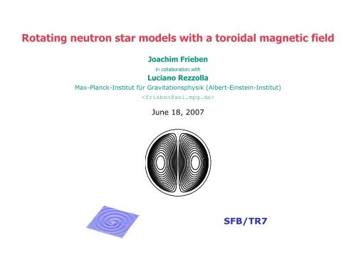
Rotating neutron star models with a toroidal magnetic field - SFB/TR7

Rotating neutron star models with a toroidal magnetic field
Joachim Frieben
in collaboration with
Luciano Rezzolla
Max-Planck-Institut für Gravitationsphysik (Albert-Einstein-Institut)
June 18, 2007
SFB/TR7

Outline
1
(1) Motivation
(2) Theoretical formulation
(3) Numerical implementation
(4) Results for an n=1 polytropic equation of state
(5) Results for realistic equations of state
(6) Conclusion
Joachim Frieben Golm, June 18, 2007

Motivation
2
Quest for astrophysical sources of gravitational radiation triggered by large scale Laser
interferometric gravitational wave detectors, such as LIGO, Virgo, or GEO600.
Potential candidates: rapidly rotating, strongly magnetized neutron stars (magnetars
beyond B ≃ 10 15 G) with a dominant toroidal field component inducing a prolate deformation
of the star.
Jones (1975): viscous processes drive the axis of symmetry orthogonal to J
=⇒ bar shaped source of gravitational waves!
Open questions:
• Prolate deformation (Q < 0) possible? Dependency
on rotation frequency f and toroidal magnetic field
strength B? Magnitude?
• Influence of general relativistic effects?
• Influence of the equation of state?
If so, for which parame-
• Configurations unstable?
ters?
Figure from Braithwaite & Spruit (2004)
Joachim Frieben Golm, June 18, 2007

Theoretical formulation
3
Assumptions: (1) space-time stationary, axisymmetric, and asymptotically flat,
(2) matter obeys circularity condition (no meridional component of momentum density
vector (massless charge carriers)), hereafter restriction to a perfect fluid.
Then: stress-energy tensor reads
T = (e+p)u ⊗ u + pg + T EM , (1)
with fluid proper energy density e, fluid pressure p, fluid four-velocity u and space-time
metric tensor g. Standard coordinates compliant with assumptions are quasi-isotropic
(polar) coordinates, conformally flat in (r,θ)-coordinate planes.
g µν d x µ d x ν = −N 2 dt 2 + B 2 r 2 sin 2 θ (dφ − N φ dt) 2 + A 2 (dr 2 + r 2 dθ 2 ) . (2)
Coordinates are global ones and cover all space. Compatibility of a purely toroidal
magnetic field with quasi-isotropic coordinates established by Oron (2002).
Electromagnetic contribution to stress energy tensor:
T EM
αβ = (1/4π)(F ακF κ β − (1/4)F κλ F κλ g αβ ) . (3)
Joachim Frieben Golm, June 18, 2007

Theoretical formulation
4
Electromagnetic contribution to (3+1) matter variables E, J, and S:
E EM = 1 (
8π
B φ
Br sinθ
Equation of stationary motion:
) 2
, J EM
i = 0 , S EMr r = S EMθ θ = −S EMφ φ = E EM . (4)
∂
1
∂xi(H + ν − lnΓ) +
e + p
1
8πB 2 N 2 r 2 sin 2 θ
∂(NB φ ) 2
∂x i = 0 . (5)
Eq. (5) only satisfied if Lorentz force term derived from a scalar function M(r,θ), hence
1 1 ∂(NB φ ) 2
e + p8πB 2 N 2 r 2 sin 2 θ ∂x i
= ∂M
∂x i . (6)
Existence of a first integral of motion established for the particular (simple) choice of
NB φ = µ(e+p) B 2 N 2 r 2 sin 2 θ , M = µ2
4π (e+p) B2 N 2 r 2 sin 2 θ . (7)
Joachim Frieben Golm, June 18, 2007

Numerical method
5
Problem: (1) sources of elliptic field equations fill all space,
(2) exact boundary condition (of asymptotic flatness) only known at spatial infinity,
(3) sources of elliptic equations involve quadratic terms of derivatives of metric
potentials themselves.
Approach: iterative procedure (relaxation) based on surface-adapted multi-domain
spectral method derived from LORENE C++ class library for numerical relativity.
Expand scalar and vector functions according to
f (r,θ) =
L∑
a l (r)coslθ , U ˜φ (r,θ) =
l=0
L∑
l=1
a ˜φ
l
(r)sinlθ . (8)
Angular expansion by Fourier series, radial expansion by Chebyshev polynomials.
Use three domains: (1) spheroidal kernel containing all the matter,
(2) intermediate domain covering the neighbourhood of the star,
(3) outer (vacuum) domain stretching to spatial infinity, mapped onto finite grid.
Code validation: (1) Full agreement with Newtonian results e.g. of Sinha (1968),
(2) for each model, error estimate provided by GRV2/GRV3 (10 −6 to 10 −10 ).
Joachim Frieben Golm, June 18, 2007

Results for an n=1 polytropic equation of state
6
Isocontours of the magnetic field
strength for a non-rotating M = 1.4 M ⊙
model with a circumferential radius of
R = 12km in the non-magnetic case. The
peak value is B p = 5.34 × 10 17 G which is
the maximum possible. Upper physical
limit for B p due to buoyancy estimated
by Wheeler (2000):
( )
B f ≃ 2 × f 1/2 ρ 1/2
×
10 13 gcm −3 × 10 18 G ,
where f ≃ 0.01. Resulting maximum
field strengths of B = 10 16 − 10 17 G.
Joachim Frieben Golm, June 18, 2007

Results for an n=1 polytropic equation of state
7
Isocontours of the magnetic potential
for the same model as on the previous
slide.
Joachim Frieben Golm, June 18, 2007

Results for an n=1 polytropic equation of state
8
Isocontours of the log-enthalpy for the
same model as on the previous slide.
Joachim Frieben Golm, June 18, 2007

Results for an n=1 polytropic equation of state
9
11.25
11
polar coordinate radius
equatorial coordinate radius
R [km]
10.75
10.5
10.25
10
Equatorial and polar radius
as a function of the peak
magnetic field strength for
a non-rotating M = 1.4 M ⊙
model with a circumferential
radius of R = 12km in
the non-magnetized case.
9.75
0 0.1 0.2 0.3 0.4 0.5 0.6 0.7 0.8 0.9 1
(B p /5.34 × 10 17 G) 2
Joachim Frieben Golm, June 18, 2007

Results for an n=1 polytropic equation of state
10
1
0.9
0.8
(Bp/5.34 × 10 17 G) 2
0.7
0.6
0.5
0.4
0.3
1
0.95
0.85
0.75 0.7
Isocontours of ratio r p /r e of polar
to equatorial radius as a function
of peak magnetic field strength
and rotation frequency for an M =
1.4 M ⊙ model with a circumferential
radius of R = 12km in the nonmagnetized
case.
0.2
0.65
0.1
0.9
0.8
0.6
0
0 0.1 0.2 0.3 0.4 0.5 0.6 0.7 0.8 0.9 1
( f /828 Hz) 2
Joachim Frieben Golm, June 18, 2007

Results for an n=1 polytropic equation of state
11
1
0.9
-0.06
-0.05
0.8
-0.04
-0.03
(Bp/5.34 × 10 17 G) 2
0.7
0.6
0.5
0.4
0.3
0.2
-0.02
-0.01
0.01
0
0.02
0.03
0.04
0.05
0.06
0.07
0.08
0.090.1
Isocontours of distortion ɛ = −3/2×
Q zz /I as a function of peak magnetic
field strength and rotation frequency
for an M = 1.4 M ⊙ model
with a circumferential radius of
R = 12km in the non-magnetized
case.
0.1
0.12 0.13
0
0.11
0.14
0 0.1 0.2 0.3 0.4 0.5 0.6 0.7 0.8 0.9 1
( f /828 Hz) 2
Joachim Frieben Golm, June 18, 2007

12
Results for an n=1 polytropic equation of state
10 −2
10 −3
10 −4
10 −5
Bonazzola & Gourgoulhon (1996)
Cutler (2002)
Magnetic distortion ɛ B as a
function of circumferential
radius R at fixed average
magnetic field strength for
a non-rotating M = 1.4 M ⊙
model computed according
to Bonazzola & Gourgoulhon
(1996) and Cutler
(2002) respectively.
−ǫ B
10 1 10 2
10 −6
R [km]
Joachim Frieben Golm, June 18, 2007

Results for realistic equations of state
13
Isocontours of the magnetic field
strength for a non-rotating M = 1.4 M ⊙
model based on the SLy4 EOS. The peak
value is B p = 2.47 × 10 17 G which is the
maximum possible.
Joachim Frieben Golm, June 18, 2007

Results for realistic equations of state
14
Isocontours of the magnetic potential
for the same model as on the previous
slide.
Joachim Frieben Golm, June 18, 2007

Results for realistic equations of state
15
Isocontours of the log-enthalpy for the
same model as on the previous slide.
Joachim Frieben Golm, June 18, 2007

Results for realistic equations of state
16
3×10 −6
2×10 −6
• BalbN1H1
• GlendNH3
• Pol2C10
2×10 −7 3×10 −7
c B Pol2F10 •
1×10 −6
• SLy4
Pol2 •
AkmalPR
BBB2 •
• FPS
• BPAL12
0
0 1×10 −7 4×10 −7
Distortion coefficients for realistic
equations of state for
models with M = 1.4 M ⊙ in the
non-rotating and non-magnetized
case. The star radius
increases as a function of the
EOS from BPAL12 bottom left
to GlendNH3 top right. Pol2
labels a relativistic model based
upon a γ = 2 polytropic
EOS with a radius of R =
12km. Pol2F10 denotes the
coefficients of a model at the
Newtonian limit with a radius
of R = 10km, Pol2C10 the
corresponding values given
by Cutler (2002).
c Ω
( ) 2 ( ) 2
¯B f
ɛ = ɛ B + ɛ Ω = −c B + c
10 15 Ω , ¯B = 〈B 2 〉 1/2 . (9)
G Hz
Joachim Frieben Golm, June 18, 2007

Conclusion
17
• First fully relativistic models of rotating stars with a toroidal magnetic field:
⋆ Only slight prolate deformation of the apparent shape.
⋆ Noticeable impact on matter distribution inside the star.
⋆ Magnetic field leads to an overall growth of the star.
⋆ For astrophysically relevant range of rotation frequency and magnetic field strength
perturbative treatment justified.
⋆ General relativistic effects attenuate the magnetic distortion.
⋆ Influence of realistic EOS dominated by impact on actual radius.
⋆ Magnetic and rotational deformation parameters given by Cutler (2002) significantly
too large.
• Further directions to explore:
⋆ Global study of neutron star models with a toroidal magnetic field.
⋆ Implement differential rotation.
⋆ Implement mixed magnetic fields (poloidal and toroidal).
⋆ Investigate instability of magnetized models.
Joachim Frieben Golm, June 18, 2007

References
18
P. B. Jones, Astrophys. Space Sci., 33, 215 (1975)
A. Oron, Phys. Rev. D 66, 023006 (2002)
http://www.lorene.obspm.fr
N. K. Sinha, Aust. J. Phys., 21, 283 (1968)
J. C. Wheeler, I. Yi, P. Höflich, and L. Wang, Astrophys. J., 537, 810 (2000)
S. Bonazzola and E. Gourgoulhon, Astron. Astrophys. 312, 675 (1996)
C. Cutler, Phys. Rev. D 66, 084025 (2002)
Golm, June 18, 2007