Exploratory Enzyme Inhibition Analysis - SigmaPlot
Exploratory Enzyme Inhibition Analysis - SigmaPlot
Exploratory Enzyme Inhibition Analysis - SigmaPlot

Create successful ePaper yourself
Turn your PDF publications into a flip-book with our unique Google optimized e-Paper software.
<strong>Exploratory</strong> <strong>Enzyme</strong> <strong>Inhibition</strong> <strong>Analysis</strong><br />
<strong>Enzyme</strong> inhibition data is analyzed with the <strong>Exploratory</strong> <strong>Enzyme</strong> Kinetics option in <strong>SigmaPlot</strong>.<br />
The direct linear plot, secondary plots and a numeric report are created to help determine if<br />
Michaelis-Menten kinetics are satisfied and to elicit the type of inhibition. This analysis provides<br />
excellent qualitative and quantitative information prior to fitting multiple candidate inhibition<br />
models using the <strong>Enzyme</strong> Kinetics module.<br />
Keywords: enzyme kinetics, inhibition, direct linear plot, secondary plots, competitive inhibition,<br />
mixed inhibition, uncompetitive inhibition, noncompetitive inhibition.<br />
Introduction<br />
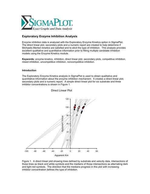
The <strong>Exploratory</strong> <strong>Enzyme</strong> Kinetics analysis in <strong>SigmaPlot</strong> is used to obtain qualitative and<br />
quantitative information about the enzyme inhibition mechanism. It creates a direct linear plot,<br />
secondary plots and a numeric report. A simple direct linear plot for six substrate and three<br />
inhibitor concentrations is shown in Figure 1.<br />
Direct Linear Plot<br />
120<br />
100<br />
Dummy Label<br />
Apparent Vmax<br />
80<br />
60<br />
40<br />
20<br />
-100 -80 -60 -40 -20 0 20 40 60<br />
Apparent Km<br />
Figure 1. A direct linear plot showing lines defined by substrate and velocity data, intersections of<br />
those lines as black and white symbols and the medians of those intersections as alternating dark<br />
and light red symbols. The direction that the medians progress in this plot with increasing<br />
inhibitor concentration defines the type of inhibition.
The <strong>Exploratory</strong> EK analysis is designed to work in conjunction with the <strong>Enzyme</strong> Kinetics module<br />
or with data entered into a <strong>SigmaPlot</strong> worksheet.<br />
An <strong>Exploratory</strong> EK <strong>Analysis</strong><br />
<strong>Enzyme</strong> inhibition data entered directly in a <strong>SigmaPlot</strong> worksheet is shown in Figure 2. There are<br />
six groups of three replicate velocity values corresponding to the six inhibitor values in column 2.<br />
Figure 2. An enzyme inhibition data set entered into a <strong>SigmaPlot</strong> worksheet. Two of six groups<br />
of replicate velocity values are shown.<br />
Running <strong>Exploratory</strong> <strong>Enzyme</strong> Kinetics displays the dialog<br />
The number of replicates is selected (this is not necessary if the analysis is run on an EK module<br />
worksheet) and then the type of plot is selected. For data sets like this one with relatively large<br />
number of substrate and inhibitor values, the Lines option is not selected since it clutters the<br />
graph and obscures the intersection and median information. Click Ok to run it. Two graph<br />
pages and a report are created.<br />
The graph pages are shown side-by-side in Figure 3 below.
180<br />
A<br />
Direct Linear Plot<br />
B<br />
0.6<br />
160<br />
140<br />
0.5<br />
Apparent Vmax<br />
120<br />
100<br />
80<br />
60<br />
Kmapp/Vmaxapp<br />
0.4<br />
0.3<br />
0.2<br />
40<br />
20<br />
0.1<br />
0<br />
0 10 20 30 40<br />
Apparent Km<br />
10 -5 0 5 10 15 20 25<br />
[Inhibitor]<br />
Michaelis-Menten Plot<br />
100<br />
0.030<br />
0.025<br />
80<br />
0.020<br />
Velocity<br />
60<br />
40<br />
1/Vmaxapp<br />
0.015<br />
0.010<br />
20<br />
0.005<br />
0<br />
0 20 40 60 80 100 120<br />
[Substrate]<br />
15 -10 -5 0 5 10 15 20 25<br />
[Inhibitor]<br />
Figure 3. Two graph pages are produced by <strong>Exploratory</strong> <strong>Enzyme</strong> Kinetics. A - the direct linear<br />
and Michaelis-Menten plots. B – the two secondary plots.<br />
These plots strongly suggest mixed inhibition since the medians progress diagonally down and to<br />
the right in the direct linear plot. Also, straight lines fit the secondary plots data very well. The<br />
two inhibition constants for mixed inhibition are the intercepts of these lines with the inhibitor axis.<br />
From the upper graph Kic = 5.1 and from the lower Kiu = 12.0.<br />
The numeric report provides median values for the direct linear and secondary plots and inhibition<br />
constant estimates from the secondary plot linear regressions – Figure 4.<br />
Figure 4. The <strong>Exploratory</strong> EK report.
A Partial Competitive <strong>Inhibition</strong> Example<br />
The Michaelis-Menten plot for simulated enzyme kinetics data is shown in Figure 5A. The direct<br />
linear plot in Figure 5B has a median trajectory that moves more-or-less horizontally from left to<br />
right suggesting a competitive inhibition (a slight decrease in apparent Vmax can be visualized so<br />
there is a possibility that this is mixed inhibition).<br />
100<br />
A<br />
140<br />
B<br />
80<br />
120<br />
Velocity<br />
60<br />
40<br />
Apparent Vmax<br />
100<br />
80<br />
60<br />
20<br />
40<br />
20<br />
0<br />
0 10 20 30 40 50 60<br />
[Substrate]<br />
0<br />
0 20 40 60 80 100 120 140<br />
Apparent Km<br />
Figure 5. Michaelis-Menten (A) and direct linear plots (B) for simulated data.<br />
The secondary plots in Figure 6 give additional information. The regression line for the apparent<br />
1/Vmax plot in Figure 6B has a slight positive slope with an inhibitor axis intercept that yields a<br />
very large inhibition constant Kiu = 1345. As seen below this is much larger than the inhibition<br />
constant Kic (=Ki) = 1.85. This slope is probably not different from zero in which case the<br />
inhibition mechanism is competitive.<br />
A<br />
1.0<br />
0.012<br />
B<br />
0.8<br />
0.010<br />
Kmapp/Vmaxapp<br />
0.6<br />
0.4<br />
median data<br />
linear regression<br />
hyperbola, y = (a + bx)/(1 + cx)<br />
1/Vmaxapp<br />
0.008<br />
0.006<br />
0.004<br />
0.2<br />
0.002<br />
40 -20 0 20 40 60 80 100 120<br />
[Inhibitor]<br />
0.000<br />
0 20 40 60 80 100 120<br />
[Inhibitor]<br />
Figure 6. Secondary plots. The apparent Km/Vmax data in Figure 6A is fit with a hyperbolic<br />
function which intersects the inhibitor axis at -Kic = -1.85.<br />
The straight line generated does not fit the apparent Km/Vmax data well. The <strong>SigmaPlot</strong><br />
hyperbolic function “Rational, 3 Parameter I” fit this data very well (R 2 = 0.999). This suggests<br />
that the inhibition mechanism is partial since partial inhibition results in hyperbolic secondary plots<br />
(hyperbolic inhibition is another name for partial inhibition).
The partial competitive inhibition parameters can be computed from the hyperbolic fit in Figure 6A<br />
as Ki = 1.85 and α = 10.5 (we are using the <strong>Enzyme</strong> Kinetics module parameter terminology<br />
where (Ki = Kic and αKi = Kiu). This compares well with the error-free simulation values Ki = 2.0<br />
and α = 10.0.<br />
A question remains as to whether the inhibition mechanism is competitive or mixed. <strong>Analysis</strong> of<br />
the initial velocity data with all equations in the Single Substrate – Single <strong>Inhibition</strong> section of the<br />
<strong>Enzyme</strong> Kinetics module produced the equation comparison shown in Table 1. The table is<br />
sorted by the Akaike criterion AICc. It separates candidate equations into groups. The<br />
competitive (partial) and mixed (partial) equations clearly form one group.<br />
The remaining equations have AICc values nearly 100 units or more higher and therefore can be<br />
removed from further consideration. The competitive (partial) equation has an AICc value 2 units<br />
less than the mixed (partial) equation and, given this data set, is the best candidate. Though the<br />
2 unit AICc difference is considered to define a difference between equations it is not a large<br />
difference, so if determining the mechanism type is important then collecting additional data is<br />
warranted.<br />
Rank by<br />
Runs<br />
AICc Equation R² AICc Sy.x Test Converg.<br />
1 Competitive (Partial) 0.98375 204.778 3.00676 pass Yes<br />
2 Mixed (Partial) 0.98379 206.845 3.02051 pass Yes<br />
3 Noncompetitive (Partial) 0.95465 297.117 5.02213 pass Yes<br />
4 Competitive (Full) 0.93093 332.741 6.16233 fail Yes<br />
5 Mixed (Full) 0.93093 334.985 6.19806 fail Yes<br />
6 Noncompetitive (Full) 0.90242 363.845 7.32470 fail Yes<br />
7 Uncompetitive (Full) 0.86781 391.170 8.52549 fail Yes<br />
8 Uncompetitive (Partial) 0.86952 392.241 8.51920 fail Yes<br />
Table 1. Comparison of <strong>Enzyme</strong> Kinetics Module single substrate-single inhibitor equation<br />
fits to simulated data.<br />
The excellent fit of the competitive (partial) equation to this data is shown in Figure 7 by the<br />
Lineweaver-Burk plot from the <strong>Enzyme</strong> Kinetics Module.<br />
1/Rate (µmol/min/mg)<br />
0.5<br />
0.4<br />
0.3<br />
0.2<br />
Vmax = 103.1<br />
Km = 10.5<br />
Ki = 2.<br />
alpha = 10.2<br />
I = 0<br />
I = 2<br />
I = 5<br />
I = 10<br />
I = 50<br />
I = 100<br />
0.1<br />
0.1 0.0 0.1 0.2 0.3 0.4 0.5 0.6<br />
1/[Substrate] (M)<br />
Figure 7. Lineweaver-Burk plot of the competitive (partial) equation fit to simulated data. Very<br />
good inhibition parameter estimates were obtained for the realistic 7% constant percentage error<br />
used.
Other Analyses<br />
One can read the article: “<strong>Exploratory</strong> <strong>Enzyme</strong> Kinetics Help” for other analysis examples.