Evaluating real integrals using the Residue Theorem - The Live Toad

EVALUATING REAL INTEGRALS
USING THE RESIDUE THEOREM
PR HEWITT
All examples taken from chapter 7 of Complex Variables and Applications,
8th edition, by James Brown and Ruel Churchill.
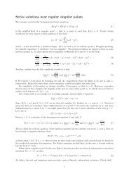
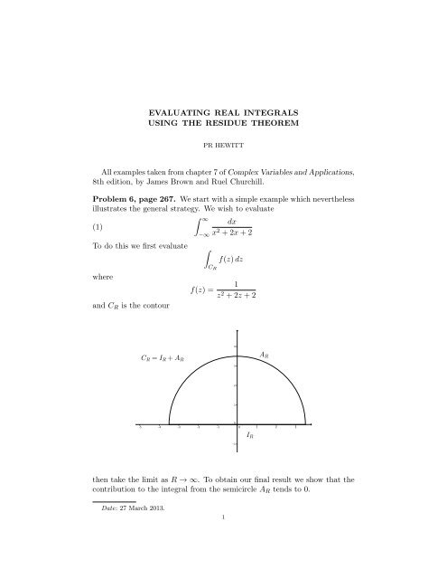
Problem 6, page 267. We start with a simple example which nevertheless
illustrates the general strategy. We wish to evaluate
(1)
To do this we first evaluate
where
and C R is the contour
∫ ∞
−∞
∫
f(z) =
dx
x 2 + 2x + 2
C R
f(z) dz
1
z 2 + 2z + 2
then take the limit as R → ∞. To obtain our final result we show that the
contribution to the integral from the semicircle A R tends to 0.
Date: 27 March 2013.
1

2 PR HEWITT
First we evaluate the contour integral using the Residue Theorem. Since
z 2 + 2z + 2 = (z + 1) 2 + 1 we see that there is exactly one singularity interior
to the contour, namely a simple pole at z = −1 + i. Hence
∫
f(z) dz = 2πi · Res f(z) = 2πi · 1
C z=−1+i R
2(−1 + i) + 2 = π
Now we need to estimate |f(z)| when |z| = R. There are several ways to do
this. Using an idea from a previous exercise we note that if z 2 +2z +2 = z 2 w
then
w = 1 + 2 z + 2 → 1 as z → ∞.
z2 Hence we may choose an R so that |w| ≥ 1 2
when |z| ≥ R. In this range we
find that
|f(z)| ≤ 1
1
≤ 2 when |z| ≥ R
2 |z|2 R2 Hence
∫
lim
R→∞
∣ f(z) dz
∣ ≤ πR · 2
A R
R 2 → 0 as R → ∞
When we put this all together we find that
∫ ∞
−∞
∫
dx
∞
x 2 + 2x + 2 = P. V.
−∞
dx
x 2 + 2x + 2
∫
= lim f(z) dz
R→∞ I
(∫
R
∫ )
= lim f(z) dz − f(z) dz
R→∞ C R A
( ∫ ) R
= lim
R→∞
π − f(z) dz
A R
= π − 0.
We can check our work directly, without recourse to complex variables,
by making the substitution u = x + 1 in (1):
∫ b
a
∫
dx
b+1
∣
x 2 + 2x + 2 = du
∣∣∣
b+1
u 2 + 1 = arctan(u)
as a → −∞ and b → +∞.
a+1
a+1
→ 1 2 π − − 1 2 π

REAL INTEGRALS AND RESIDUES 3
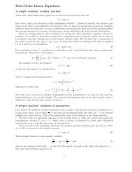
Problem 8, pages 267–268. We are asked to evaluate
(2)
∫ ∞
0
dx
x 3 + 1
The book suggests taking f(z) = 1/(z 3 + 1) and integrating f along the
contour
This will proceed along the same lines as above, using the Residue Theorem
and demonstrating that the contribution to the integral from the circular arc
tends to 0. The main difference is the extra segment J R : the contribution
from this segment is significant, and so we must parametrize it carefully and
study the integral there.
Again there is only one singularity inside the contour, and that is a simple
pole at e iπ/3 . Hence
∫
C R
f(z) dz = 2πi ·
Res f(z) = 2πi ·
z=e iπ/3
1
3(e iπ/3 ) 2 = i 2 2π/3
3πe−i When |z| = R > 1 the Triangle Inequality tells us that
1
|f(z)| ≤
R 3 − 1
whence ∣∫
∣∣∣ f(z) dz
∣ ≤ 2 3 πR · 1
A R
R 3 → 0 as R → ∞.
− 1
Now the new and interesting bit. Along J R we take the parametrization
z = re i 2π/3 for 0 ≤ r ≤ R. This parametrizes J R backwards, hence
∫
∫
∫ R
e i 2π/3 ∫
dr
f(z) dz = − f(z) dz = −
J R −J R 0 r 3 + 1
= −ei 2π/3 f(z) dz.
I R

4 PR HEWITT
When we put all this together we find that
i 2 3 πe−i 2π/3 = (1 − e i 2π/3 )
∫
f(z) dz +
I R
∫
f(z) dz.
A R
If we take the limit as R → ∞ and divide both sides by 1 − e i 2π/3 we
conclude that
∫ ∞
0
dx
x 3 + 1 =
i 2π
3(e i 2π/3 − e −i 2π/3 ) = π
3 sin(2π/3) = 2π
3 √ 3
This integral can also be done without recourse to the Residue Theorem,
by factoring x 3 + 1 as (x + 1)(x 2 − x + 1) and then applying the standard
techniques from Callc II — partial fractions, trig substitution, etc. I will
leave this as an exercise.
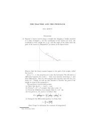
Problem 7, page 276. We now do a simple application of Jordan’s Lemma.
We are asked to evaluate
(3)
∫ ∞
−∞
x sin x dx
(x 2 + 1)(x 2 + 4)
Notice that the integrand is even. Hence
We take
∫ ∞
−∞
∫
x sin x dx
∞
(x 2 + 1)(x 2 + 4) = Im P. V.
f(z) =
−∞
z
(z 2 + 1)(z 2 + 4)
x e ix dx
(x 2 + 1)(x 2 + 4)
and integrate f(z)e iz over the contour below and apply Jordan’s Lemma to
the integral over the semicircle.

REAL INTEGRALS AND RESIDUES 5
Inside this contour there are two singularities, simple poles at i and 2i.
Hence
∫
(
)
f(z)e iz dz = 2πi · Res
C z=i f(z)eiz + Res
z=2i f(z)eiz R
(
ie −1
= 2πi ·
2i · (−1 + 4) + 2ie −2 )
(−4 + 1) · 4i
π(e − 1)
= i
3e 2 .
When |z| = R > 2 we find that
R
|f(z)| ≤
(R 2 − 1)(R 2 → 0 as R → ∞.
− 4)
Hence by Jordan’s Lemma we have
∫
f(z)e iz dz → 0 as R → ∞.
A R
If we put this all together then we conclude
∫ ∞
∫
x sin x dx
−∞ (x 2 + 1)(x 2 = Im lim f(z)e iz dz
+ 4) R→∞ I
(∫
R
∫
)
= Im lim f(z)e iz dz − f(z)e iz dz
R→∞ C R A R
π(e − 1)
= Im(i
3e 2 − 0)
π(e − 1)
=
3e 2

6 PR HEWITT
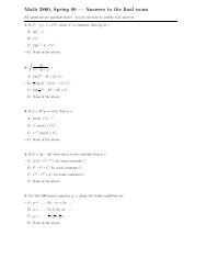
Problem 1, page 286. We are asked to evaluate
∫ ∞
cos(ax) − cos(bx)
(4)
0 x 2 dx
Note that
cos(az)
z 2 = 1 z 2 − a 2 + · · ·
and thus
cos(az) − cos(bz)
z 2 = b − a + · · ·
2
which is entire! There will be no residues to compute if we integrate this
function.
Instead we integrate
f(z) = eiaz − e ibz
z 2 = i a − b + · · · ,
z
which has a simple pole at 0, and then look at the real part. The complication
is that this function is singular at a point along the natural contour
for this problem — in fact the improper integral near 0 diverges. So we
take an “indented contour” to ensure that the integrand is analytic along
the contour:
By the Residue Theorem we have that
∫
C R
f(z) dz = 0.
Since 1/|z| 2 = 1/R 2 along A R Jordan’s Lemma (applied twice) tells us
that
∫
A R
f(z) dz → 0 as R → ∞

REAL INTEGRALS AND RESIDUES 7
Along J we take the parametrization z = −x for ρ ≤ x ≤ R and find that
∫
∫
∫ R
e −iax − e −ibx
f(z) dz = − f(z) dz = −
(−dx)
Hence
J
∫
I+J
−J
ρ
x 2
∫ R
cos(ax) − cos(bx)
f(z) dz = 2
ρ x 2 dx
It remains to study what happens to the integral along Γ ρ as ρ → 0. Here
we meet an old friend in a new guise. Let us consider a slightly more general
situation. Suppose that g(z) has a simple pole at z 0 with residue B, and we
integrate g along circular arc of small radius ρ:
Near z 0 we have that
g(z) =
B
z − z 0
+ h(z)
where h(z) is analytic. For sufficiently small ρ we have (say)
|h(z)| ≤ |h(z 0 )| + 1
whence
∫
h(z) dz
∣ Γ ρ
∣ ≤ (β − α)ρ · (|h(z 0)| + 1) → 0 as ρ → 0
This yields
∫
lim
ρ→0
∫ β
g(z) dz = lim
Γ ρ ρ→0 α
B · iρe iθ dθ
ρe iθ
∫
+ lim h(z) dz = i (β − α)B
ρ→0 Γ ρ
When α = 0 and β = 2π we recover the essential computation in the proof of
the Residue Theorem. In our case we have α = π, β = 0, and B = i(a − b).

8 PR HEWITT
If we put all this together then we obtain
∫ ∞
∫
cos(ax) − cos(bx)
1
0 x 2 dx = lim
ρ→0, R→∞ 2
∫
1
= − lim
ρ→0 2
I+J
f(z) dz
Γ ρ
f(z) dz − lim
R→∞
= − 1 2i (−π) · i (a − b) − 0
Problem 3, page 286. We are asked to use the function
to evaluate the integrals
(5)
f(z) = z1/3 log z
z 2 + 1
, − 1 2 π < arg z < 3 2 π
∫ ∞
0
3√ ∫ x ln x
∞ 3√ x
x 2 + 1 dx and x 2 + 1 dx
0
∫
1
f(z) dz
2 A R
Two for the price of one! As with the previous example we will use what
the text calls an “indented contour”, but in this case we will be eschewing
a branch cut, not an isolated singularity. The limit calculations will be very
different for the indentation.
We use the same contour as above:
When R is large and ρ is small the enclosed region contains exactly one
singularity, namely a simple pole at i. Hence
∫
C
f(z) dz = 2πi · Res
z=i f(z) = 2πi · i1/3 log i
2i
= i π2
2 eiπ/6

REAL INTEGRALS AND RESIDUES 9
Now we need to estimate the contributions to the integral from A and Γ.
When |z| = r we find that
Hence
and
|f(z)| ≤ r1/3 (| ln r| + 3 2 π)
|r 2 − 1|
∫
∣ f(z) dz
∣ ≤ πR · R1/3 (ln R + 3 2 π)
A R
R 2 → 0 as R → +∞
− 1
∣ ∣∣∣∣ ∫
f(z) dz
Γ ρ
∣ ≤ πρ · ρ1/3 (− ln ρ + 3 2 π)
1 − ρ 2 → 0 as ρ → 0 +
by L’Hospital’s Rule.
Thus, in the limit, all of the action is along I and J. We can parametrize
J backwards using z = −x for ρ ≤ x ≤ R. Along this segment we have that
−x = e iπ x. Thus
∫
J
∫
f(z) dz = −
−J
= e iπ/3 ∫ R
ρ
∫ R
e iπ/3 3√ x (ln x + iπ)
f(z) dz = −
ρ x 2 + 1
3√ x ln x
x 2 + 1 dx + i πeiπ/3 ∫ R
ρ
3√ x
x 2 + 1 dx
When we put all these integrals together we find that
∫ ∫
∫ ∫
i π2
2 eiπ/6 = f(z) dz + f(z) dz + f(z) dz +
I
= (1 + e iπ/3 )
J
∫ R
ρ
∫
+ f(z) dz +
Γ
0
Γ
3√ ∫ x ln x
R
x 2 + 1 dx + i πeiπ/3 ρ
∫
f(z) dz
A
A
(−dx)
f(z) dz
3√ x
x 2 + 1 dx
If we take limits as ρ → 0 and R → +∞, then divide both sides by e iπ/6
then we obtain
∫ ∞ 3√ ∫
i π2
x ln x
∞ 3√ x
2 = 2 cos(π/6) x 2 + 1 dx + i πeiπ/6 x 2 + 1 dx
If we look at the real and imaginary parts of the above equation we find
that
√
∫ ∞ 3√ x ln x
3
0 x 2 + 1 dx = π ∫ ∞ 3√ x
2 0 x 2 + 1 dx
π 2
2 = π√ ∫
3 ∞ 3√ x
2 x 2 + 1 dx
which lead to the answers given in the text.
0
0

10 PR HEWITT
Problem 6, page 291. Finally we show how we can sometimes use residues
to evaluate ordinary (that is, not improper) integrals by making a substitution
that transforms the real integral into a contour integral. For example,
to compute
(6)
∫ π
0
dθ
(a + cos θ) n , a > 1.
we use the substitution
Thus
where
z = e iθ , dz = i e iθ dz = iz dz, cos θ = 1 2 (z + z−1 ).
∫ π
0
dθ
(a + cos θ) n = 1 ∫ 2π
dθ
2 0 (a + cos θ) n
= 1 ∫
dz
2 iz(a + 1 2 (z + z−1 )) n
= 2n−1
i
= 2n−1
i
|z|=1
∫
∫
|z|=1
|z|=1
r, s = −a ± √ a 2 − 1.
z n−1 dz
(z 2 + 2az + 1) n
z n−1 dz
(z − r) n (z − s) n
Since r < −1 we find that the only singularity in the circle is a pole of order
n is the root s = 1/r. Thus
∫ π
0
dθ
(a + cos θ) n = z n−1
2n π · Res
z=s (z − r) n (z − s) n
We expand z n−1 /(z − r) n in a Laurent series around s:
z n−1 (z − s + s)n−1
=
(z − r) n (s − r + z − s) n
=
n−1
1 ∑
(s − r) n
×
j=0
( n − 1
j
∞∑
( ) −n (z − s)
k
k (s − r) k
k=0
)
s j (z − s) n−1−j

Hence
∫ π
dθ
(a + cos θ) n = 2n n−1
π ∑
(s − r) n
0
REAL INTEGRALS AND RESIDUES 11
l=0
( n − 1
= 2n n−1
π ∑
( n − 1
(s − r) n l
=
l=0
2 n n−1
π ∑
(s − r) 2n−1
l=0
l
( n − 1
)( −n
l
) ( s
s − r
)( n + l − 1
l
) l
) l
) ( −s
l s − r
)( ) n + l − 1
(−s) l (s − r) n−l−1
l
Note that −s = a − √ a 2 − 1 and s − r = 2 √ a 2 − 1. Thus when n = 2 we
obtain
4π
(
8(a 2 − 1) 3/2 2 √ a 2 − 1 + 2(a − √ )
a 2 πa
− 1) =
(a 2 − 1) 3/2
When n = 3 we obtain
8π
(
32(a 2 − 1) 5/2 4(a 2 − 1) + 6(a − √ a 2 − 1) · 2 √ a 2 − 1 + 6(a − √ a 2 − 1) 2)
What is the pattern for arbitrary n?
= π(4a2 + 2)
4(a 2 − 1) 5/2