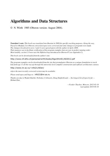
Algorithms and Data Structures

Algorithms and Data Structures 

© N. Wirth 1985 (Oberon version: August 2004). 

Translator's note. This book was translated into Russian in 2009 for specific teaching purposes. Along the way, 

Pascal-to-Modula-2-to-Oberon conversion typos were corrected and some changes to programs were made. 

The changes (localized in sects. 1 and 3) were agreed upon with the author in April, 2009. 

Their purpose was to facilitate verification of the program examples that are now in perfect running order. 

Most notably, section 1.9 now uses the Dijkstra loop introduced in Oberon-07 (see Appendix C). 

This book can be downloaded from the author's site: 

http://www.inf.ethz.ch/personal/wirth/books/AlgorithmE1/AD2012.pdf 

The program examples can be downloaded from the site that promulgates Oberons as a unique foundation to teach 

kids from age 11 all the way up through the university-level compiler construction and software architecture courses: 

http://www.inr.ac.ru/~info21/ADen/ 

where the most recently corrected version may be available. 

Please send typos and bugs to: info21@inr.ac.ru 

Thanks are due to Wojtek Skulski, Nicholas J. Schwartz, Doug Danforth and — the longest list of typos by far — 

Helmut Zinn. 

—Fyodor Tkachov, Moscow, 2012-02-18 

Last update 2014-04-10

N.Wirth. Algorithms and Data Structures. Oberon version 2 

Table of Contents 

Preface 

Preface To The 1985 Edition 

Notation 

1 Fundamental Data Structures 10 

1.1 Introduction 

1.2 The Concept of Data Type 

1.3 Standard Primitive Types 

1.3.1 The type INTEGER 

1.3.2 The type REAL 

1.3.3 The type BOOLEAN 

1.3.4 The type CHAR 

1.3.5 The type SET 

1.4 The Array Structure 

1.5 The Record Structure 

1.6 Representation of Arrays, Records, and Sets 

1.6.1 Representation of Arrays 

1.6.2 Representation of Records 

1.6.3 Representation of Sets 

1.7 The File (Sequence) 

1.7.1 Elementary File Operators 

1.7.2 Buffering Sequences 

1.7.3 Buffering between Concurrent Processes 

1.7.4 Textual Input and Output 

1.8 Searching 

1.8.1 Linear Search 

1.8.2 Binary Search 

1.8.3 Table Search 

1.9 String Search 

1.9.1 Straight String Search 

1.9.2 The Knuth-Morris-Pratt String Search 

1.9.3 The Boyer-Moore String Search 

Exercises 

References 

2 Sorting 50 


2.2 Sorting Arrays 

2.2.1 Sorting by Straight Insertion 

2.2.2 Sorting by Straight Selection 

2.2.3 Sorting by Straight Exchange 

2.3 Advanced Sorting Methods 

2.3.1 Insertion Sort by Diminishing Increment 

2.3.2 Tree Sort 

2.3.3 Partition Sort 

2.3.4 Finding the Median


2.3.5 A Comparison of Array Sorting Methods 

2.4 Sorting Sequences 

2.4.1 Straight Merging 

2.4.2 Natural Merging 

2.4.3 Balanced Multiway Merging 

2.4.4 Polyphase Sort 

2.4.5 Distribution of Initial Runs 

Exercises 

References 

3 Recursive Algorithms 99 


3.2 When Not to Use Recursion 

3.3 Two Examples of Recursive Programs 

3.4 Backtracking Algorithms 

3.5 The Eight Queens Problem 

3.6 The Stable Marriage Problem 

3.7 The Optimal Selection Problem 

Exercises 

References 

4 Dynamic Information Structures 129 

4.1 Recursive Data Types 

4.2 Pointers 

4.3 Linear Lists 

4.3.1 Basic Operations 

4.3.2 Ordered Lists and Reorganizing Lists 

4.3.3 An Application: Topological Sorting 

4.4 Tree Structures 

4.4.1 Basic Concepts and Definitions 

4.4.2 Basic Operations on Binary Trees 

4.4.3 Tree Search and Insertion 

4.4.4 Tree Deletion 


4.5 Balanced Trees 

4.5.1 Balanced Tree Insertion 

4.5.2 Balanced Tree Deletion 

4.6 Optimal Search Trees 

4.7 B-Trees 

4.7.1 Multiway B-Trees 

4.7.2 Binary B-Trees 

4.8 Priority Search Trees 

Exercises 

References 

5 Key Transformations (Hashing) 200 


5.2 Choice of a Hash Function 

5.3 Collision handling


5.4 Analysis of Key Transformation 

Exercises 

References 

Appendices 207 

A. The ASCII Character Set 

B. The Syntax of Oberon 

C. The Dijkstra loop 

Index


Preface 

In recent years the subject of computer programming has been recognized as a discipline whose mastery 

is fundamental and crucial to the success of many engineering projects and which is amenable to scientific 

treatement and presentation. It has advanced from a craft to an academic discipline. The initial outstanding 

contributions toward this development were made by E.W. Dijkstra and C.A.R. Hoare. Dijkstra's Notes 

on Structured Programming [1] opened a new view of programming as a scientific subject and 

intellectual challenge, and it coined the title for a "revolution" in programming. Hoare's Axiomatic Basis of 

Computer Programming [2] showed in a lucid manner that programs are amenable to an exacting 

analysis based on mathematical reasoning. Both these papers argue convincingly that many programming 

errors can be prevented by making programmers aware of the methods and techniques which they hitherto 

applied intuitively and often unconsciously. These papers focused their attention on the aspects of 

composition and analysis of programs, or more explicitly, on the structure of algorithms represented by 

program texts. Yet, it is abundantly clear that a systematic and scientific approach to program construction 

primarily has a bearing in the case of large, complex programs which involve complicated sets of data. 

Hence, a methodology of programming is also bound to include all aspects of data structuring. Programs, 

after all, are concrete formulations of abstract algorithms based on particular representations and structures 

of data. An outstanding contribution to bring order into the bewildering variety of terminology and concepts 

on data structures was made by Hoare through his Notes on Data Structuring [3]. It made clear that 

decisions about structuring data cannot be made without knowledge of the algorithms applied to the data 

and that, vice versa, the structure and choice of algorithms often depend strongly on the structure of the 

underlying data. In short, the subjects of program composition and data structures are inseparably 

interwined. 

Yet, this book starts with a chapter on data structure for two reasons. First, one has an intuitive feeling 

that data precede algorithms: you must have some objects before you can perform operations on them. 

Second, and this is the more immediate reason, this book assumes that the reader is familiar with the basic 

notions of computer programming. Traditionally and sensibly, however, introductory programming courses 

concentrate on algorithms operating on relatively simple structures of data. Hence, an introductory chapter 

on data structures seems appropriate. 

Throughout the book, and particularly in Chap. 1, we follow the theory and terminology expounded by 

Hoare and realized in the programming language Pascal [4]. The essence of this theory is that data in the 

first instance represent abstractions of real phenomena and are preferably formulated as abstract structures 

not necessarily realized in common programming languages. In the process of program construction the 

data representation is gradually refined in step with the refinement of the algorithm to comply more and 

more with the constraints imposed by an available programming system [5]. We therefore postulate a 

number of basic building principles of data structures, called the fundamental structures. It is most important 

that they are constructs that are known to be quite easily implementable on actual computers, for only in 

this case can they be considered the true elements of an actual data representation, as the molecules 

emerging from the final step of refinements of the data description. They are the record, the array (with 

fixed size), and the set. Not surprisingly, these basic building principles correspond to mathematical notions 

that are fundamental as well. 

A cornerstone of this theory of data structures is the distinction between fundamental and "advanced" 

structures. The former are the molecules themselves built out of atoms that are the components of the 

latter. Variables of a fundamental structure change only their value, but never their structure and never the 

set of values they can assume. As a consequence, the size of the store they occupy remains constant.


"Advanced" structures, however, are characterized by their change of value and structure during the 

execution of a program. More sophisticated techniques are therefore needed for their implementation. The 

sequence appears as a hybrid in this classification. It certainly varies its length; but that change in structure 

is of a trivial nature. Since the sequence plays a truly fundamental role in practically all computer systems, 

its treatment is included in Chap. 1. 

The second chapter treats sorting algorithms. It displays a variety of different methods, all serving the 

same purpose. Mathematical analysis of some of these algorithms shows the advantages and disadvantages 

of the methods, and it makes the programmer aware of the importance of analysis in the choice of good 

solutions for a given problem. The partitioning into methods for sorting arrays and methods for sorting files 

(often called internal and external sorting) exhibits the crucial influence of data representation on the choice 

of applicable algorithms and on their complexity. The space allocated to sorting would not be so large were 

it not for the fact that sorting constitutes an ideal vehicle for illustrating so many principles of programming 

and situations occurring in most other applications. It often seems that one could compose an entire 

programming course by choosing examples from sorting only. 

Another topic that is usually omitted in introductory programming courses but one that plays an 

important role in the conception of many algorithmic solutions is recursion. Therefore, the third chapter is 

devoted to recursive algorithms. Recursion is shown to be a generalization of repetition (iteration), and as 

such it is an important and powerful concept in programming. In many programming tutorials, it is 

unfortunately exemplified by cases in which simple iteration would suffice. Instead, Chap. 3 concentrates 

on several examples of problems in which recursion allows for a most natural formulation of a solution, 

whereas use of iteration would lead to obscure and cumbersome programs. The class of backtracking 

algorithms emerges as an ideal application of recursion, but the most obvious candidates for the use of 

recursion are algorithms operating on data whose structure is defined recursively. These cases are treated 

in the last two chapters, for which the third chapter provides a welcome background. 

Chapter 4 deals with dynamic data structures, i.e., with data that change their structure during the 

execution of the program. It is shown that the recursive data structures are an important subclass of the 

dynamic structures commonly used. Although a recursive definition is both natural and possible in these 

cases, it is usually not used in practice. Instead, the mechanism used in its implementation is made evident 

to the programmer by forcing him to use explicit reference or pointer variables. This book follows this 

technique and reflects the present state of the art: Chapter 4 is devoted to programming with pointers, to 

lists, trees and to examples involving even more complicated meshes of data. It presents what is often (and 

somewhat inappropriately) called list processing. A fair amount of space is devoted to tree organizations, 

and in particular to search trees. The chapter ends with a presentation of scatter tables, also called "hash" 

codes, which are often preferred to search trees. This provides the possibility of comparing two 

fundamentally different techniques for a frequently encountered application. 

Programming is a constructive activity. How can a constructive, inventive activity be taught? One 

method is to crystallize elementary composition priciples out many cases and exhibit them in a systematic 

manner. But programming is a field of vast variety often involving complex intellectual activities. The belief 

that it could ever be condensed into a sort of pure recipe teaching is mistaken. What remains in our arsenal 

of teaching methods is the careful selection and presentation of master examples. Naturally, we should not 

believe that every person is capable of gaining equally much from the study of examples. It is the 

characteristic of this approach that much is left to the student, to his diligence and intuition. This is 

particularly true of the relatively involved and long example programs. Their inclusion in this book is not 

accidental. Longer programs are the prevalent case in practice, and they are much more suitable for 

exhibiting that elusive but essential ingredient called style and orderly structure. They are also meant to 

serve as exercises in the art of program reading, which too often is neglected in favor of program writing. 

This is a primary motivation behind the inclusion of larger programs as examples in their entirety. The


reader is led through a gradual development of the program; he is given various snapshots in the evolution 

of a program, whereby this development becomes manifest as a stepwise refinement of the details. I 

consider it essential that programs are shown in final form with sufficient attention to details, for in 

programming, the devil hides in the details. Although the mere presentation of an algorithm's principle and 

its mathematical analysis may be stimulating and challenging to the academic mind, it seems dishonest to the 

engineering practitioner. I have therefore strictly adhered to the rule of presenting the final programs in a 

language in which they can actually be run on a computer. 

Of course, this raises the problem of finding a form which at the same time is both machine executable and 

sufficiently machine independent to be included in such a text. In this respect, neither widely used languages 

nor abstract notations proved to be adequate. The language Pascal provides an appropriate compromise; it 

had been developed with exactly this aim in mind, and it is therefore used throughout this book. The 

programs can easily be understood by programmers who are familiar with some other high-level language, 

such as ALGOL 60 or PL/1, because it is easy to understand the Pascal notation while proceeding through 

the text. However, this not to say that some proparation would not be beneficial. The book Systematic 

Programming [6] provides an ideal background because it is also based on the Pascal notation. The 

present book was, however, not intended as a manual on the language Pascal; there exist more appropriate 

texts for this purpose [7]. 

This book is a condensation and at the same time an elaboration of several courses on programming 

taught at the Federal Institute of Technology (ETH) at Zürich. I owe many ideas and views expressed in 

this book to discussions with my collaborators at ETH. In particular, I wish to thank Mr. H. Sandmayr for 

his careful reading of the manuscript, and Miss Heidi Theiler and my wife for their care and patience in 

typing the text. I should also like to mention the stimulating influence provided by meetings of the Working 

Groups 2.1 and 2.3 of IFIP, and particularly the many memorable arguments I had on these occasions with 

E. W. Dijkstra and C.A.R. Hoare. Last but not least, ETH generously provided the environment and the 

computing facilities without which the preparation of this text would have been impossible. 

Zürich, Aug. 1975 

N. Wirth 

[1] E.W. Dijkstra, in: O.-J. Dahl, E.W. Dijkstra, C.A.R. Hoare. Structured Programming. F. Genuys, 

Ed., New York, Academic Press, 1972, pp. 1-82. 

[2] C.A.R. Hoare. Comm. ACM, 12, No. 10 (1969), 576-83. 

[3] C.A.R. Hoare, in Structured Programming [1], cc. 83-174. 

[4] N. Wirth. The Programming Language Pascal. Acta Informatica, 1, No. 1 (1971), 35-63. 

[5] N. Wirth. Program Development by Stepwise Refinement. Comm. ACM, 14, No. 4 (1971), 221-27. 

[6] N. Wirth. Systematic Programming. Englewood Cliffs, N.J. Prentice-Hall, Inc., 1973. 

[7] K. Jensen and N. Wirth. PASCAL-User Manual and Report. Berlin, Heidelberg, New York; 

Springer-Verlag, 1974.


Preface To The 1985 Edition 

This new Edition incorporates many revisions of details and several changes of more significant nature. 

They were all motivated by experiences made in the ten years since the first Edition appeared. Most of the 

contents and the style of the text, however, have been retained. We briefly summarize the major alterations. 

The major change which pervades the entire text concerns the programming language used to express the 

algorithms. Pascal has been replaced by Modula-2. Although this change is of no fundamental influence to 

the presentation of the algorithms, the choice is justified by the simpler and more elegant syntactic 

structures of Modula-2, which often lead to a more lucid representation of an algorithm's structure. Apart 

from this, it appeared advisable to use a notation that is rapidly gaining acceptance by a wide community, 

because it is well-suited for the development of large programming systems. Nevertheless, the fact that 

Pascal is Modula's ancestor is very evident and eases the task of a transition. The syntax of Modula is 

summarized in the Appendix for easy reference. 

As a direct consequence of this change of programming language, Sect. 1.11 on the sequential file 

structure has been rewritten. Modula-2 does not offer a built-in file type. The revised Sect. 1.11 presents 

the concept of a sequence as a data structure in a more general manner, and it introduces a set of program 

modules that incorporate the sequence concept in Modula-2 specifically. 

The last part of Chapter 1 is new. It is dedicated to the subject of searching and, starting out with linear 

and binary search, leads to some recently invented fast string searching algorithms. In this section in 

particular we use assertions and loop invariants to demonstrate the correctness of the presented algorithms. 

A new section on priority search trees rounds off the chapter on dynamic data structures. Also this 

species of trees was unknown when the first Edition appeared. They allow an economical representation 

and a fast search of point sets in a plane. 

The entire fifth chapter of the first Edition has been omitted. It was felt that the subject of compiler 

construction was somewhat isolated from the preceding chapters and would rather merit a more extensive 

treatment in its own volume. 

Finally, the appearance of the new Edition reflects a development that has profoundly influenced 

publications in the last ten years: the use of computers and sophisticated algorithms to prepare and 

automatically typeset documents. This book was edited and laid out by the author with the aid of a Lilith 

computer and its document editor Lara. Without these tools, not only would the book become more 

costly, but it would certainly not be finished yet. 

Palo Alto, March 1985 

N. Wirth


Notation 

The following notations, adopted from publications of E.W. Dijkstra, are used in this book. 

In logical expressions, the character & denotes conjunction and is pronounced as and. The character ~ 

denotes negation and is pronounced as not. Boldface A and E are used to denote the universal and 

existential quantifiers. In the following formulas, the left part is the notation used and defined here in terms 

of the right part. Note that the left parts avoid the use of the symbol "...", which appeals to the readers 

intuition. 

Ai: m ≤ i < n : P i P m & P m+1 & ... & P n-1 

The P i are predicates, and the formula asserts that for all indices i ranging from a given value m to, but 

excluding a value n P i holds. 

Ei: m ≤ i < n : P i P m or P m+1 or ... or P n-1 

The P i are predicates, and the formula asserts that for some indices i ranging from a given value m to, but 

excluding a value n P i holds. 

Si: m ≤ i < n : x i = x m + x m+1 + ... + x n-1 

MIN i: m ≤ i < n : x i = minimum(x m , ... , x n-1 ) 

MAX i: m ≤ i < n : x i = maximum(x m , ... , x n-1 )


1 Fundamental Data Structures 


The modern digital computer was invented and intended as a device that should facilitate and speed up 

complicated and time-consuming computations. In the majority of applications its capability to store and 

access large amounts of information plays the dominant part and is considered to be its primary 

characteristic, and its ability to compute, i.e., to calculate, to perform arithmetic, has in many cases become 

almost irrelevant. 

In all these cases, the large amount of information that is to be processed in some sense represents an 

abstraction of a part of reality. The information that is available to the computer consists of a selected set of 

data about the actual problem, namely that set that is considered relevant to the problem at hand, that set 

from which it is believed that the desired results can be derived. The data represent an abstraction of reality 

in the sense that certain properties and characteristics of the real objects are ignored because they are 

peripheral and irrelevant to the particular problem. An abstraction is thereby also a simplification of facts. 

We may regard a personnel file of an employer as an example. Every employee is represented 

(abstracted) on this file by a set of data relevant either to the employer or to his accounting procedures. 

This set may include some identification of the employee, for example, his or her name and salary. But it 

will most probably not include irrelevant data such as the hair color, weight, and height. 

In solving a problem with or without a computer it is necessary to choose an abstraction of reality, i.e., 

to define a set of data that is to represent the real situation. This choice must be guided by the problem to 

be solved. Then follows a choice of representation of this information. This choice is guided by the tool that 

is to solve the problem, i.e., by the facilities offered by the computer. In most cases these two steps are not 

entirely separable. 

The choice of representation of data is often a fairly difficult one, and it is not uniquely determined by the 

facilities available. It must always be taken in the light of the operations that are to be performed on the 

data. A good example is the representation of numbers, which are themselves abstractions of properties of 

objects to be characterized. If addition is the only (or at least the dominant) operation to be performed, 

then a good way to represent the number n is to write n strokes. The addition rule on this representation is 

indeed very obvious and simple. The Roman numerals are based on the same principle of simplicity, and 

the adding rules are similarly straightforward for small numbers. On the other hand, the representation by 

Arabic numerals requires rules that are far from obvious (for small numbers) and they must be memorized. 

However, the situation is reversed when we consider either addition of large numbers or multiplication and 

division. The decomposition of these operations into simpler ones is much easier in the case of 

representation by Arabic numerals because of their systematic structuring principle that is based on 

positional weight of the digits. 

It is generally known that computers use an internal representation based on binary digits (bits). This 

representation is unsuitable for human beings because of the usually large number of digits involved, but it is 

most suitable for electronic circuits because the two values 0 and 1 can be represented conveniently and 

reliably by the presence or absence of electric currents, electric charge, or magnetic fields. 

From this example we can also see that the question of representation often transcends several levels of 

detail. Given the problem of representing, say, the position of an object, the first decision may lead to the 

choice of a pair of real numbers in, say, either Cartesian or polar coordinates. The second decision may 

lead to a floating-point representation, where every real number x consists of a pair of integers denoting a 

fraction f and an exponent e to a certain base (such that x = f × 2 e ). The third decision, based on the


knowledge that the data are to be stored in a computer, may lead to a binary, positional representation of 

integers, and the final decision could be to represent binary digits by the electric charge in a semiconductor 

storage device. Evidently, the first decision in this chain is mainly influenced by the problem situation, and 

the later ones are progressively dependent on the tool and its technology. Thus, it can hardly be required 

that a programmer decide on the number representation to be employed, or even on the storage device 

characteristics. These lower-level decisions can be left to the designers of computer equipment, who have 

the most information available on current technology with which to make a sensible choice that will be 

acceptable for all (or almost all) applications where numbers play a role. 

In this context, the significance of programming languages becomes apparent. A programming language 

represents an abstract computer capable of interpreting the terms used in this language, which may embody 

a certain level of abstraction from the objects used by the actual machine. Thus, the programmer who uses 

such a higher-level language will be freed (and barred) from questions of number representation, if the 

number is an elementary object in the realm of this language. 

The importance of using a language that offers a convenient set of basic abstractions common to most 

problems of data processing lies mainly in the area of reliability of the resulting programs. It is easier to 

design a program based on reasoning with familiar notions of numbers, sets, sequences, and repetitions 

than on bits, storage units, and jumps. Of course, an actual computer represents all data, whether numbers, 

sets, or sequences, as a large mass of bits. But this is irrelevant to the programmer as long as he or she 

does not have to worry about the details of representation of the chosen abstractions, and as long as he or 

she can rest assured that the corresponding representation chosen by the computer (or compiler) is 

reasonable for the stated purposes. 

The closer the abstractions are to a given computer, the easier it is to make a representation choice for 

the engineer or implementor of the language, and the higher is the probability that a single choice will be 

suitable for all (or almost all) conceivable applications. This fact sets definite limits on the degree of 

abstraction from a given real computer. For example, it would not make sense to include geometric objects 

as basic data items in a general-purpose language, since their proper repesentation will, because of its 

inherent complexity, be largely dependent on the operations to be applied to these objects. The nature and 

frequency of these operations will, however, not be known to the designer of a general-purpose language 

and its compiler, and any choice the designer makes may be inappropriate for some potential applications. 

In this book these deliberations determine the choice of notation for the description of algorithms and 

their data. Clearly, we wish to use familiar notions of mathematics, such as numbers, sets, sequences, and 

so on, rather than computer-dependent entities such as bitstrings. But equally clearly we wish to use a 

notation for which efficient compilers are known to exist. It is equally unwise to use a closely machineoriented 

and machine-dependent language, as it is unhelpful to describe computer programs in an abstract 

notation that leaves problems of representation widely open. The programming language Pascal had been 

designed in an attempt to find a compromise between these extremes, and the successor languages 

Modula-2 and Oberon are the result of decades of experience [1-3]. Oberon retains Pascal's basic 

concepts and incorporates some improvements and some extensions; it is used throughout this book [1-5]. 

It has been successfully implemented on several computers, and it has been shown that the notation is 

sufficiently close to real machines that the chosen features and their representations can be clearly 

explained. The language is also sufficiently close to other languages, and hence the lessons taught here may 

equally well be applied in their use. 

1.2 The Concept of Data Type 

In mathematics it is customary to classify variables according to certain important characteristics. Clear 

distinctions are made between real, complex, and logical variables or between variables representing 

individual values, or sets of values, or sets of sets, or between functions, functionals, sets of functions, and


so on. This notion of classification is equally if not more important in data processing. We will adhere to the 

principle that every constant, variable, expression, or function is of a certain type. This type essentially 

characterizes the set of values to which a constant belongs, or which can be assumed by a variable or 

expression, or which can be generated by a function. 

In mathematical texts the type of a variable is usually deducible from the typeface without consideration 

of context; this is not feasible in computer programs. Usually there is one typeface available on computer 

equipment (i.e., Latin letters). The rule is therefore widely accepted that the associated type is made 

explicit in a declaration of the constant, variable, or function, and that this declaration textually precedes 

the application of that constant, variable, or function. This rule is particularly sensible if one considers the 

fact that a compiler has to make a choice of representation of the object within the store of a computer. 

Evidently, the amount of storage allocated to a variable will have to be chosen according to the size of the 

range of values that the variable may assume. If this information is known to a compiler, so-called dynamic 

storage allocation can be avoided. This is very often the key to an efficient realization of an algorithm. 

The primary characteristics of the concept of type that is used throughout this text, and that is embodied 

in the programming language Oberon, are the following [1-2]: 

1. A data type determines the set of values to which a constant belongs, or which may be assumed by a 

variable or an expression, or which may be generated by an operator or a function. 

2. The type of a value denoted by a constant, variable, or expression may be derived from its form or its 

declaration without the necessity of executing the computational process. 

3. Each operator or function expects arguments of a fixed type and yields a result of a fixed type. If an 

operator admits arguments of several types (e.g., + is used for addition of both integers and real 

numbers), then the type of the result can be determined from specific language rules. 

As a consequence, a compiler may use this information on types to check the legality of various 

constructs. For example, the mistaken assignment of a Boolean (logical) value to an arithmetic variable may 

be detected without executing the program. This kind of redundancy in the program text is extremely useful 

as an aid in the development of programs, and it must be considered as the primary advantage of good 

high-level languages over machine code (or symbolic assembly code). Evidently, the data will ultimately be 

represented by a large number of binary digits, irrespective of whether or not the program had initially been 

conceived in a high-level language using the concept of type or in a typeless assembly code. To the 

computer, the store is a homogeneous mass of bits without apparent structure. But it is exactly this abstract 

structure which alone is enabling human programmers to recognize meaning in the monotonous landscape 

of a computer store. 

The theory presented in this book and the programming language Oberon specify certain methods of 

defining data types. In most cases new data types are defined in terms of previously defined data types. 

Values of such a type are usually conglomerates of component values of the previously defined constituent 

types, and they are said to be structured. If there is only one constituent type, that is, if all components are 

of the same constituent type, then it is known as the base type. The number of distinct values belonging to a 

type T is called its cardinality. The cardinality provides a measure for the amount of storage needed to 

represent a variable x of the type T, denoted by x: T. 

Since constituent types may again be structured, entire hierarchies of structures may be built up, but, 

obviously, the ultimate components of a structure are atomic. Therefore, it is necessary that a notation is 

provided to introduce such primitive, unstructured types as well. A straightforward method is that of 

enumerating the values that are to constitute the type. For example in a program concerned with plane 

geometric figures, we may introduce a primitive type called shape, whose values may be denoted by the 

identifiers rectangle, square, ellipse, circle. But apart from such programmer-defined types, there will


have to be some standard, predefined types. They usually include numbers and logical values. If an 

ordering exists among the individual values, then the type is said to be ordered or scalar. In Oberon, all 

unstructured types are ordered; in the case of explicit enumeration, the values are assumed to be ordered 

by their enumeration sequence. 

With this tool in hand, it is possible to define primitive types and to build conglomerates, structured types 

up to an arbitrary degree of nesting. In practice, it is not sufficient to have only one general method of 

combining constituent types into a structure. With due regard to practical problems of representation and 

use, a general-purpose programming language must offer several methods of structuring. In a mathematical 

sense, they are equivalent; they differ in the operators available to select components of these structures. 

The basic structuring methods presented here are the array, the record, the set, and the sequence. More 

complicated structures are not usually defined as static types, but are instead dynamically generated during 

the execution of the program, when they may vary in size and shape. Such structures are the subject of 

Chap. 4 and include lists, rings, trees, and general, finite graphs. 

Variables and data types are introduced in a program in order to be used for computation. To this end, 

a set of operators must be available. For each standard data type a programming languages offers a certain 

set of primitive, standard operators, and likewise with each structuring method a distinct operation and 

notation for selecting a component. The task of composition of operations is often considered the heart of 

the art of programming. However, it will become evident that the appropriate composition of data is 

equally fundamental and essential. 

The most important basic operators are comparison and assignment, i.e., the test for equality (and for 

order in the case of ordered types), and the command to enforce equality. The fundamental difference 

between these two operations is emphasized by the clear distinction in their denotation throughout this text. 

Test for equality: x = y (an expression with value TRUE or FALSE) 

Assignment to x: x := y (a statement making x equal to y) 

These fundamental operators are defined for most data types, but it should be noted that their execution 

may involve a substantial amount of computational effort, if the data are large and highly structured. 

For the standard primitive data types, we postulate not only the availability of assignment and 

comparison, but also a set of operators to create (compute) new values. Thus we introduce the standard 

operations of arithmetic for numeric types and the elementary operators of propositional logic for logical 

values. 

1.3 Standard Primitive Types 

Standard primitive types are those types that are available on most computers as built-in features. They 

include the whole numbers, the logical truth values, and a set of printable characters. On many computers 

fractional numbers are also incorporated, together with the standard arithmetic operations. We denote 

these types by the identifiers 

INTEGER, REAL, BOOLEAN, CHAR, SET 

1.3.1 The type INTEGER 

The type INTEGER comprises a subset of the whole numbers whose size may vary among individual 

computer systems. If a computer uses n bits to represent an integer in two's complement notation, then the 

admissible values x must satisfy -2 n-1 ≤ x < 2 n-1 . It is assumed that all operations on data of this type are 

exact and correspond to the ordinary laws of arithmetic, and that the computation will be interrupted in the 

case of a result lying outside the representable subset. This event is called overflow. The standard 

operators are the four basic arithmetic operations of addition (+), subtraction (-), multiplication (*) and


division (/, DIV). 

Whereas the slash denotes ordinary division resulting in a value of type REAL, the operator DIV denotes 

integer division resulting in a value of type INTEGER. If we define the quotient q = m DIV n and the 

remainder r = m MOD n, the following relations hold, assuming n > 0: 

q*n + r = m and 0 ≤ r < n 

Examples 

31 DIV 10 = 3 31 MOD 10 = 1 

-31 DIV 10 = -4 -31 MOD 10 = 9 

We know that dividing by 10 n can be achieved by merely shifting the decimal digits n places to the right 

and thereby ignoring the lost digits. The same method applies, if numbers are represented in binary instead 

of decimal form. If two's complement representation is used (as in practically all modern computers), then 

the shifts implement a division as defined by the above DIV operaton. Moderately sophisticated compilers 

will therefore represent an operation of the form m DIV 2 n or m MOD 2 n by a fast shift (or mask) 

operation. 

1.3.2 The type REAL 

The type REAL denotes a subset of the real numbers. Whereas arithmetic with operands of the types 

INTEGER is assumed to yield exact results, arithmetic on values of type REAL is permitted to be inaccurate 

within the limits of round-off errors caused by computation on a finite number of digits. This is the principal 

reason for the explicit distinction between the types INTEGER and REAL, as it is made in most programming 

languages. 

The standard operators are the four basic arithmetic operations of addition (+), subtraction (-), 

multiplication (*), and division (/). It is an essence of data typing that different types are incompatible under 

assignment. An exception to this rule is made for assignment of integer values to real variables, because 

here the semanitcs are unambiguous. After all, integers form a subset of real numbers. However, the 

inverse direction is not permissible: Assignment of a real value to an integer variable requires an operation 

such as truncation or rounding. The standard transfer function ENTIER(x) yields the integral part of x. 

Rounding of x is obtained by ENTIER(x + 0.5). 

Many programming languages do not include an exponentiation operator. The following is an algorithm 

for the fast computation of y = x n , where n is a non-negative integer. 

y := 1.0; i := n; (* ADenS13 *) 

WHILE i > 0 DO (* x 0 n = x i * y *) 

IF ODD(i) THEN y := y*x END; 

x := x*x; i := i DIV 2 

END


1.3.3 The type BOOLEAN 

The two values of the standard type BOOLEAN are denoted by the identifiers TRUE and FALSE. The 

Boolean operators are the logical conjunction, disjunction, and negation whose values are defined in Table 

1.1. The logical conjunction is denoted by the symbol &, the logical disjunction by OR, and negation by "~". 

Note that comparisons are operations yielding a result of type BOOLEAN. Thus, the result of a comparison 

may be assigned to a variable, or it may be used as an operand of a logical operator in a Boolean 

expression. For instance, given Boolean variables p and q and integer variables x = 5, y = 8, z = 10, the 

two assignments 

p := x = y 

q := (x ≤ y) & (y < z) 

yield p = FALSE and q = TRUE. 

p q p OR q p & q ~p 

TRUE TRUE TRUE TRUE FALSE 

TRUE FALSE TRUE FALSE FALSE 

FALSE TRUE TRUE FALSE TRUE 

FALSE FALSE FALSE FALSE TRUE 

Table 1.1. Boolean Operators. 

The Boolean operators & (AND) and OR have an additional property in most programming languages, 

which distinguishes them from other dyadic operators. Whereas, for example, the sum x+y is not defined, if 

either x or y is undefined, the conjunction p&q is defined even if q is undefined, provided that p is FALSE. 

This conditionality is an important and useful property. The exact definition of & and OR is therefore given 

by the following equations: 

p & q = if p then q else FALSE 

p OR q = if p then TRUE else q 

1.3.4 The type CHAR 

The standard type CHAR comprises a set of printable characters. Unfortunately, there is no generally 

accepted standard character set used on all computer systems. Therefore, the use of the predicate 

"standard" may in this case be almost misleading; it is to be understood in the sense of "standard on the 

computer system on which a certain program is to be executed." 

The character set defined by the International Standards Organization (ISO), and particularly its 

American version ASCII (American Standard Code for Information Interchange) is the most widely 

accepted set. The ASCII set is therefore tabulated in Appendix A. It consists of 95 printable (graphic) 

characters and 33 control characters, the latter mainly being used in data transmission and for the control of 

printing equipment. 

In order to be able to design algorithms involving characters (i.e., values of type CHAR), that are system 

independent, we should like to be able to assume certain minimal properties of character sets, namely: 

1. The type CHAR contains the 26 capital Latin letters, the 26 lower-case letters, the 10 decimal digits, and 

a number of other graphic characters, such as punctuation marks. 

2. The subsets of letters and digits are ordered and contiguous, i.e.,


("A" ≤ x) & (x ≤ "Z") 

("a" ≤ x) & (x ≤ "z") 

implies that x is a capital letter 

implies that x is a lower-case letter 

("0" ≤ x) & (x ≤ "9") implies that x is a decimal digit 

3. The type CHAR contains a non-printing, blank character and a line-end character that may be used as 

separators. 

THIS IS A TEXT 

Fig. 1.1. Representations of a text 

The availability of two standard type transfer functions between the types CHAR and INTEGER is 

particularly important in the quest to write programs in a machine independent form. We will call them 

ORD(ch), denoting the ordinal number of ch in the character set, and CHR(i), denoting the character with 

ordinal number i. Thus, CHR is the inverse function of ORD, and vice versa, that is, 

ORD(CHR(i)) = i (if CHR(i) is defined) 

CHR(ORD(c)) 

= c 

Furthermore, we postulate a standard function CAP(ch). Its value is defined as the capital letter 

corresponding to ch, provided ch is a letter. 

ch is a lower-case letter implies that 

ch is a capital letter implies that 

CAP(ch) = corresponding capital letter 

CAP(ch) = ch 

1.3.5 The type SET 

The type SET denotes sets whose elements are integers in the range 0 to a small number, typically 31 or 

63. Given, for example, variables 

VAR r, s, t: SET 

possible assignments are 

r := {5}; s := {x, y .. z}; t := {} 

Here, the value assigned to r is the singleton set consisting of the single element 5; to t is assigned the 

empty set, and to s the elements x, y, y+1, … , z-1, z. 

The following elementary operators are defined on variables of type SET: 

* set intersection 

+ set union 

- set difference 

/ symmetric set difference 

IN set membership 

Constructing the intersection or the union of two sets is often called set multiplication or set addition, 

respectively; the priorities of the set operators are defined accordingly, with the intersection operator 

having priority over the union and difference operators, which in turn have priority over the membership


operator, which is classified as a relational operator. Following are examples of set expressions and their 

fully parenthesized equivalents: 

r * s + t 

r - s * t 

r - s + t 

r + s / t 

= (r*s) + t 

= r - (s*t) 

= (r-s) + t 

= r + (s/t) 

x IN s + t = x IN (s+t) 

1.4 The Array Structure 

The array is probably the most widely used data structure; in some languages it is even the only one 

available. An array consists of components which are all of the same type, called its base type; it is 

therefore called a homogeneous structure. The array is a random-access structure, because all 

components can be selected at random and are equally quickly accessible. In order to denote an individual 

component, the name of the entire structure is augmented by the index selecting the component. This index 

is to be an integer between 0 and n-1, where n is the number of elements, the size, of the array. 

TYPE T = ARRAY n OF T0 

Examples 

TYPE Row 

TYPE Card 

TYPE Name 

= ARRAY 4 OF REAL 

= ARRAY 80 OF CHAR 

= ARRAY 32 OF CHAR 

A particular value of a variable 

VAR x: Row 

with all components satisfying the equation x i = 2 -i , may be visualized as shown in Fig. 1.2. 

x 0 

x 1 

x 2 

x 3 

1.0 

0.5 

0.25 

0.125 

Fig. 1.2. Array of type Row with x i = 2 -i . 

An individual component of an array can be selected by an index. Given an array variable x, we denote 

an array selector by the array name followed by the respective component's index i, and we write x i or 

x[i]. Because of the first, conventional notation, a component of an array component is therefore also 

called a subscripted variable. 

The common way of operating with arrays, particularly with large arrays, is to selectively update single 

components rather than to construct entirely new structured values. This is expressed by considering an 

array variable as an array of component variables and by permitting assignments to selected components, 

such as for example x[i] := 0.125. Although selective updating causes only a single component value to 

change, from a conceptual point of view we must regard the entire composite value as having changed too. 

The fact that array indices, i.e., names of array components, are integers, has a most important 

consequence: indices may be computed. A general index expression may be substituted in place of an 

index constant; this expression is to be evaluated, and the result identifies the selected component. This


generality not only provides a most significant and powerful programming facility, but at the same time it 

also gives rise to one of the most frequently encountered programming mistakes: The resulting value may be 

outside the interval specified as the range of indices of the array. We will assume that decent computing 

systems provide a warning in the case of such a mistaken access to a non-existent array component. 

The cardinality of a structured type, i. e. the number of values belonging to this type, is the product of the 

cardinality of its components. Since all components of an array type T are of the same base type T0, we 

obtain 

card(T) 

= card(T0) n 

Constituents of array types may themselves be structured. An array variable whose components are 

again arrays is called a matrix. For example, 

M: ARRAY 10 OF Row 

is an array consisting of ten components (rows), each constisting of four components of type REAL. and is 

called a 10 x 4 matrix with real components. Selectors may be concatenated accordingly, such that M ij and 

M[i][j] denote the j-th component of row M i , which is the i-th component of M. This is usually abbreviated 

as M[i,j], and in the same spirit the declaration 

M: ARRAY 10 OF ARRAY 4 OF REAL 

can be written more concisely as 

M: ARRAY 10, 4 OF REAL 

If a certain operation has to be performed on all components of an array or on adjacent components of 

a section of the array, then this fact may conveniently be emphasized by using the FOR satement, as shown 

in the following examples for computing the sum and for finding the maximal element of an array declared 

as 

VAR a: ARRAY N OF INTEGER; (* ADenS14 *) 

sum := 0; 

FOR i := 0 TO N-1 DO sum := a[i] + sum END 

k := 0; max := a[0]; 

FOR i := 1 TO N-1 DO 

IF max < a[i] THEN k := i; max := a[k] END 

END 

In a further example, assume that a fraction f is represented in its decimal form with k-1 digits, i.e., by an 

array d such that 

f = Si: 0 ≤ i < k: d i * 10 -i 

f = d 0 + 10*d 1 + 100*d 2 + … + 10 k-1 *d k-1 

Now assume that we wish to divide f by 2. This is done by repeating the familiar division operation for all 

k-1 digits d i , starting with i=1. It consists of dividing each digit by 2 taking into account a possible carry 

from the previous position, and of retaining a possible remainder r for the next position: 

r := 10*r +d[i]; d[i] := r DIV 2; r := r MOD 2 

This algorithm is used to compute a table of negative powers of 2. The repetition of halving to compute 2 - 

1 , 2 -2 , ... , 2 -N is again appropriately expressed by a FOR statement, thus leading to a nesting of two FOR 

statements.


PROCEDURE Power (VAR W: Texts.Writer; N: INTEGER); (* ADenS14 *) 

(*compute decimal representation of negative powers of 2*) 

VAR i, k, r: INTEGER; 

d: ARRAY N OF INTEGER; 

BEGIN 

FOR k := 0 TO N-1 DO 

Texts.Write(W, "."); r := 0; 

FOR i := 0 TO k-1 DO 

r := 10*r + d[i]; d[i] := r DIV 2; r := r MOD 2; 

Texts.Write(W, CHR(d[i] + ORD("0"))) 

END; 

d[k] := 5; Texts.Write(W, "5"); Texts.WriteLn(W) 

END 

END Power 

The resulting output text for N = 10 is 

.5 

.25 

.125 

.0625 

.03125 

.015625 

.0078125 

.00390625 

.001953125 

.0009765625 

1.5 The Record Structure 

The most general method to obtain structured types is to join elements of arbitrary types, that are 

possibly themselves structured types, into a compound. Examples from mathematics are complex numbers, 

composed of two real numbers, and coordinates of points, composed of two or more numbers according 

to the dimensionality of the space spanned by the coordinate system. An example from data processing is 

describing people by a few relevant characteristics, such as their first and last names, their date of birth, 

sex, and marital status. 

In mathematics such a compound type is the Cartesian product of its constituent types. This stems from 

the fact that the set of values defined by this compound type consists of all possible combinations of values, 

taken one from each set defined by each constituent type. Thus, the number of such combinations, also 

called n-tuples, is the product of the number of elements in each constituent set, that is, the cardinality of 

the compound type is the product of the cardinalities of the constituent types. 

In data processing, composite types, such as descriptions of persons or objects, usually occur in files or 

data banks and record the relevant characteristics of a person or object. The word record has therefore 

become widely accepted to describe a compound of data of this nature, and we adopt this nomenclature in 

preference to the term Cartesian product. In general, a record type T with components of the types T 1 , T 2 , 

... , T n is defined as follows: 

TYPE T = RECORD s 1 : T 1 ; s 2 : T 2 ; ... s n : T n END 

card(T) = card(T 1 ) * card(T 2 ) * ... * card(T n )


Examples 

TYPE Complex = RECORD re, im: REAL END 

TYPE Date = RECORD day, month, year: INTEGER END 

TYPE Person = RECORD name, firstname: Name; 

birthdate: Date; 

male: BOOLEAN 

END 

We may visualize particular, record-structured values of, for example, the variables 

z: Complex 

d: Date 

p: Person 

as shown in Fig. 1.3. 

Complex z 

Date d 

Person p 

1.0 

-1.0 

1 

4 

1973 

SMITH 

JOHN 

18 1 1986 

TRUE 

Fig. 1.3. Records of type Complex, Date and Person. 

The identifiers s 1 , s 2 , ... , s n introduced by a record type definition are the names given to the individual 

components of variables of that type. As components of records are called fields, the names are field 

identifiers. They are used in record selectors applied to record structured variables. Given a variable x: T, 

its i-th field is denoted by x.s i . Selective updating of x is achieved by using the same selector denotation 

on the left side in an assignment statement: 

x.s i := e 

where e is a value (expression) of type T i . Given, for example, the record variables z, d, and p declared 

above, the following are selectors of components: 

z.im 

d.month 

p.name 

p.birthdate 

p.birthdate.day 

p.mail 

(of type REAL) 

(of type INTEGER) 

(of type Name) 

(of type Date) 

(of type INTEGER) 

(of type BOOLEAN) 

The example of the type Person shows that a constituent of a record type may itself be structured. Thus, 

selectors may be concatenated. Naturally, different structuring types may also be used in a nested fashion. 

For example, the i-th component of an array a being a component of a record variable r is denoted by 

r.a[i], and the component with the selector name s of the i-th record structured component of the array a 

is denoted by a[i].s. 

It is a characteristic of the Cartesian product that it contains all combinations of elements of the 

constituent types. But it must be noted that in practical applications not all of them may be meaningful. For 

instance, the type Date as defined above includes the 31st April as well as the 29th February 1985, which 

are both dates that never occurred. Thus, the definition of this type does not mirror the actual situation


entirely correctly; but it is close enough for practical purposes, and it is the responsibility of the programmer 

to ensure that meaningless values never occur during the execution of a program. 

The following short excerpt from a program shows the use of record variables. Its purpose is to count 

the number of persons represented by the array variable family that are both female and born after the year 

2000: 

VAR 

count: INTEGER; 

family: ARRAY N OF Person; 

count := 0; 


IF ~family[i].male & (family[i].birthdate.year > 2000) THEN INC(count) END 

END 

The record structure and the array structure have the common property that both are random-access 

structures. The record is more general in the sense that there is no requirement that all constituent types 

must be identical. In turn, the array offers greater flexibility by allowing its component selectors to be 

computable values (expressions), whereas the selectors of record components are field identifiers declared 

in the record type definition. 

1.6 Representation Of Arrays, Records, And Sets 

The essence of the use of abstractions in programming is that a program may be conceived, understood, 

and verified on the basis of the laws governing the abstractions, and that it is not necessary to have further 

insight and knowledge about the ways in which the abstractions are implemented and represented in a 

particular computer. Nevertheless, it is essential for a professional programmer to have an understanding of 

widely used techniques for representing the basic concepts of programming abstractions, such as the 

fundamental data structures. It is helpful insofar as it might enable the programmer to make sensible 

decisions about program and data design in the light not only of the abstract properties of structures, but 

also of their realizations on actual computers, taking into account a computer's particular capabilities and 

limitations. 

The problem of data representation is that of mapping the abstract structure onto a computer store. 

Computer stores are — in a first approximation — arrays of individual storage cells called bytes. They are 

understood to be groups of 8 bits. The indices of the bytes are called addresses. 

VAR store: ARRAY StoreSize OF BYTE 

The basic types are represented by a small number of bytes, typically 2, 4, or 8. Computers are 

designed to transfer internally such small numbers (possibly 1) of contiguous bytes concurrently, "in 

parallel". The unit transferable concurrently is called a word. 

1.6.1 Representation of Arrays 

A representation of an array structure is a mapping of the (abstract) array with components of type T 

onto the store which is an array with components of type BYTE. The array should be mapped in such a 

way that the computation of addresses of array components is as simple (and therefore as efficient) as 

possible. The address i of the j-th array component is computed by the linear mapping function 

i = i 0 + j*s, 

where i 0 is the address of the first component, and s is the number of words that a component occupies. 

Assuming that the word is the smallest individually transferable unit of store, it is evidently highly desirable 

that s be a whole number, the simplest case being s = 1. If s is not a whole number (and this is the normal


case), then s is usually rounded up to the next larger integer S. Each array component then occupies S 

words, whereby S-s words are left unused (see Figs. 1.4 and 1.5). Rounding up of the number of words 

needed to the next whole number is called padding. The storage utilization factor u is the quotient of the 

minimal amounts of storage needed to represent a structure and of the amount actually used: 

u = s / (s rounded up to nearest integer) 

i 0 

store 

array 

Fig. 1.4. Mapping an array onto a store 

s=2.3 

S=3 

unused 

Fig. 1.5. Padded representation of a record 

Since an implementor has to aim for a storage utilization as close to 1 as possible, and since accessing 

parts of words is a cumbersome and relatively inefficient process, he or she must compromise. The 

following considerations are relevant: 

1. Padding decreases storage utilization. 

2. Omission of padding may necessitate inefficient partial word access. 

3. Partial word access may cause the code (compiled program) to expand and therefore to counteract 

the gain obtained by omission of padding. 

In fact, considerations 2 and 3 are usually so dominant that compilers always use padding automatically. 

We notice that the utilization factor is always u > 0.5, if s > 0.5. However, if s ≤ 0.5, the utilization factor 

may be significantly increased by putting more than one array component into each word. This technique is 

called packing. If n components are packed into a word, the utilization factor is (see Fig. 1.6) 

u = n*s / (n*s rounded up to nearest integer) 

padded 

Fig. 1.6. Packing 6 components into one word 

Access to the i-th component of a packed array involves the computation of the word address j in which 

the desired component is located, and it involves the computation of the respective component position k 

within the word. 

j = i DIV n 

k = i MOD n 

In most programming languages the programmer is given no control over the representation of the abstract


data structures. However, it should be possible to indicate the desirability of packing at least in those cases 

in which more than one component would fit into a single word, i.e., when a gain of storage economy by a 

factor of 2 and more could be achieved. We propose the convention to indicate the desirability of packing 

by prefixing the symbol ARRAY (or RECORD) in the declaration by the symbol PACKED. 

1.6.2 Representation of Records 

Records are mapped onto a computer store by simply juxtaposing their components. The address of a 

component (field) r i relative to the origin address of the record r is called the field's offset k i . It is computed 

as 

k i = s 1 + s 2 + ... + s i-1 k 0 = 0 

where s j is the size (in words) of the j-th component. We now realize that the fact that all components of an 

array are of equal type has the welcome consequence that k i = i × s. The generality of the record 

structure does unfortunately not allow such a simple, linear function for offset address computation, and it is 

therefore the very reason for the requirement that record components be selectable only by fixed 

identifiers. This restriction has the desirable benefit that the respective offsets are known at compile time. 

The resulting greater efficiency of record field access is well-known. 

The technique of packing may be beneficial, if several record components can be fitted into a single 

storage word (see Fig. 1.7). Since offsets are computable by the compiler, the offset of a field packed 

within a word may also be determined by the compiler. This means that on many computers packing of 

records causes a deterioration in access efficiency considerably smaller than that caused by the packing of 

arrays. 

s 1 

s 2 s 3 

s 4 

padded 

s 5 

s 6 s 7 s 8 

Fig. 1.7. Representation of a packed record 

1.6.3 Representation of Sets 

A set s is conveniently represented in a computer store by its characteristic function C(s). This is an 

array of logical values whose ith component has the meaning "i is present in s". As an example, the set of 

small integers s = {2, 3, 5, 7, 11, 13} is represented by the sequence of bits, by a bitstring: 

C(s) = (… 0010100010101100) 

The representation of sets by their characteristic function has the advantage that the operations of 

computing the union, intersection, and difference of two sets may be implemented as elementary logical 

operations. The following equivalences, which hold for all elements i of the base type of the sets x and y, 

relate logical operations with operations on sets: 

i IN (x+y) = (i IN x) OR (i IN y) 

i IN (x*y) = (i IN x) & (i IN y) 

i IN (x-y) = (i IN x) & ~(i IN y)


These logical operations are available on all digital computers, and moreover they operate concurrently on 

all corresponding elements (bits) of a word. It therefore appears that in order to be able to implement the 

basic set operations in an efficient manner, sets must be represented in a small, fixed number of words 

upon which not only the basic logical operations, but also those of shifting are available. Testing for 

membership is then implemented by a single shift and a subsequent (sign) bit test operation. As a 

consequence, a test of the form x IN {c 1 , c 2 , ... , c n } can be implemented considerably more efficiently 

than the equivalent Boolean expression 

(x = c 1 ) OR (x = c 2 ) OR ... OR (x = c n ) 

A corollary is that the set structure should be used only for small integers as elements, the largest one being 

the wordlength of the underlying computer (minus 1). 

1.7 The File (Sequence) 

Another elementary structuring method is the sequence. A sequence is typically a homogeneous 

structure like the array. That is, all its elements are of the same type, the base type of the sequence. We 

shall denote a sequence s with n elements by 

s = 

n is called the length of the sequence. This structure looks exactly like the array. The essential difference is 

that in the case of the array the number of elements is fixed by the array's declaration, whereas for the 

sequence it is left open. This implies that it may vary during execution of the program. Although every 

sequence has at any time a specific, finite length, we must consider the cardinality of a sequence type as 

infinite, because there is no fixed limit to the potential length of sequence variables. 

A direct consequence of the variable length of sequences is the impossibility to allocate a fixed amount 

of storage to sequence variables. Instead, storage has to be allocated during program execution, namely 

whenever the sequence grows. Perhaps storage can be reclaimed when the sequence shrinks. In any case, 

a dynamic storage allocation scheme must be employed. All structures with variable size share this 

property, which is so essential that we classify them as advanced structures in contrast to the fundamental 

structures discussed so far. 

What, then, causes us to place the discussion of sequences in this chapter on fundamental structures? 

The primary reason is that the storage management strategy is sufficiently simple for sequences (in contrast 

to other advanced structures), if we enforce a certain discipline in the use of sequences. In fact, under this 

proviso the handling of storage can safely be delegated to a machanism that can be guaranteed to be 

reasonably effective. The secondary reason is that sequences are indeed ubiquitous in all computer 

applications. This structure is prevalent in all cases where different kinds of storage media are involved, i.e. 

where data are to be moved from one medium to another, such as from disk or tape to primary store or 

vice-versa. 

The discipline mentioned is the restraint to use sequential access only. By this we mean that a sequence 

is inspected by strictly proceeding from one element to its immediate successor, and that it is generated by 

repeatedly appending an element at its end. The immediate consequence is that elements are not directly 

accessible, with the exception of the one element which currently is up for inspection. It is this accessing 

discipline which fundamentally distinguishes sequences from arrays. As we shall see in Chapter 2, the 

influence of an access discipline on programs is profound. 

The advantage of adhering to sequential access which, after all, is a serious restriction, is the relative 

simplicity of needed storage management. But even more important is the possibility to use effective 

buffering techniques when moving data to or from secondary storage devices. Sequential access allows us 

to feed streams of data through pipes between the different media. Buffering implies the collection of 

sections of a stream in a buffer, and the subsequent shipment of the whole buffer content once the buffer is


filled. This results in very significantly more effective use of secondary storage. Given sequential access 

only, the buffering mechanism is reasonably straightforward for all sequences and all media. It can therefore 

safely be built into a system for general use, and the programmer need not be burdened by incorporating it 

in the program. Such a system is usually called a file system, because the high-volume, sequential access 

devices are used for permanent storage of (persistent) data, and they retain them even when the computer 

is switched off. The unit of data on these media is commonly called (sequential) file. Here we will use the 

term file as synonym to sequence. 

There exist certain storage media in which the sequential access is indeed the only possible one. Among 

them are evidently all kinds of tapes. But even on magnetic disks each recording track constitutes a storage 

facility allowing only sequential access. Strictly sequential access is the primary characteristic of every 

mechanically moving device and of some other ones as well. 

It follows that it is appropriate to distinguish between the data structure, the sequence, on one hand, 

and the mechanism to access elements on the other hand. The former is declared as a data structure, the 

latter typically by the introduction of a record with associated operators, or, according to more modern 

terminology, by a rider object. The distinction between data and mechanism declarations is also useful in 

view of the fact that several access points may exist concurrently on one and the same sequence, each one 

representing a sequential access at a (possibly) different location. 

We summarize the essence of the foregoing as follows: 

1. Arrays and records are random access structures. They are used when located in primary, randomaccess 

store. 

2. Sequences are used to access data on secondary, sequential-access stores, such as disks and tapes. 

3. We distinguish between the declaration of a sequence variable, and that of an access mechanism 

located at a certain position within the seqence. 

1.7.1 Elementary File Operators 

The discipline of sequential access can be enforced by providing a set of seqencing operators through 

which files can be accessed exclusively. Hence, although we may here refer to the i-th element of a 

sequence s by writing s i , this shall not be possible in a program. 

Sequences, files, are typically large, dynamic data structures stored on a secondary storage device. Such 

a device retains the data even if a program is terminated, or a computer is switched off. Therefore the 

introduction of a file variable is a complex operation connecting the data on the external device with the file 

variable in the program. We therefore define the type File in a separate module, whose definition specifies 

the type together with its operators. We call this module Files and postulate that a sequence or file variable 

must be explicitly initialized (opened) by calling an appropriate operator or function: 

VAR f: File 

f := Open(name) 

where name identifies the file as recorded on the persistent data carrier. Some systems distinguish between 

opening an existing file and opening a new file: 

f := Old(name) 

f := New(name) 

The disconnection between secondary storage and the file variable then must also be explicitly requested 

by, for example, a call of Close(f). 

Evidently, the set of operators must contain an operator for generating (writing) and one for inspecting 

(reading) a sequence. We postulate that these operations apply not to a file directly, but to an object called 

a rider, which itself is connected with a file (sequence), and which implements a certain access mechanism. 

The sequential access discipline is guaranteed by a restrictive set of access operators (procedures).


A sequence is generated by appending elements at its end after having placed a rider on the file. 

Assuming the declaration 

VAR r: Rider 

we position the rider r on the file f by the statement 

Set(r, f, pos) 

where pos = 0 designates the beginning of the file (sequence). A typical pattern for generating the 

sequence is: 

WHILE more DO compute next element x; Write(r, x) END 

A sequence is inspected by first positioning a rider as shown above, and then proceeding from element to 

element. A typical pattern for reading a sequence is: 

Read(r, x); 

WHILE ~r.eof DO process element x; Read(r, x) END 

Evidently, a certain position is always associated with every rider. It is denoted by r.pos. Furthermore, 

we postulate that a rider contain a predicate (flag) r.eof indicating whether a preceding read operation had 

reached the sequence's end. We can now postulate and describe informally the following set of primitive 

operators: 

1a. New(f, name) defines f to be the empty sequence. 

1b. Old(f, name) defines f to be the sequence persistently stored with given name. 

2. Set(r, f, pos) associate rider r with sequence f, and place it at position pos. 

3. Write(r, x) place element with value x in the sequence designated by rider r, and advance. 

4. Read(r, x) assign to x the value of the element designated by rider r, and advance. 

5. Close(f) registers the written file f in the persistent store (flush buffers). 

Note. Writing an element in a sequence is often a complex operation. However, mostly, files are created 

by appending elements at the end. 

Translator's note. The program examples in the book use two more commands: 

6. WriteInt(r, n) place the integer n in the sequence designated by rider r, and advance. 

7. ReadInt(r, n) assign to n the integer value designated by rider r, and advance. 

In order to convey a more precise understanding of the sequencing operators, the following example of 

an implementation is provided. It shows how they might be expressed if sequences were represented by 

arrays. This example of an implementation intentionally builds upon concepts introduced and discussed 

earlier, and it does not involve either buffering or sequential stores which, as mentioned above, make the 

sequence concept truly necessary and attractive. Nevertheless, this example exhibits all the essential 

characteristics of the primitive sequence operators, independently of how the sequences are represented in 

store. 

The operators are presented in terms of conventional procedures. This collection of definitions of types, 

variables, and procedure headings (signatures) is called a definition. We assume that we are to deal with 

sequences of characters, i.e. text files whose elements are of type CHAR. The declarations of File and Rider 

are good examples of an application of record structures because, in addition to the field denoting the array 

which represents the data, further fields are required to denote the current length and position, i.e. the state 

of the rider.


DEFINITION Files; (* ADenS171_Files *) 

TYPE File; (*sequence of characters*) 

Rider = RECORD eof: BOOLEAN END; 

PROCEDURE New(VAR name: ARRAY OF CHAR): File; 

PROCEDURE Old(VAR name: ARRAY OF CHAR): File; 

PROCEDURE Close(VAR f: File); 

PROCEDURE Set(VAR r: Rider; VAR f: File; pos: INTEGER); 

PROCEDURE Write(VAR r: Rider; ch: CHAR); 

PROCEDURE Read(VAR r: Rider; VAR ch: CHAR); 

PROCEDURE WriteInt(VAR r: Rider; n: INTEGER); 

PROCEDURE ReadInt(VAR r: Rider; VAR n: INTEGER); 

END Files. 

A definition represents an abstraction. Here we are given the two data types, File and Rider, together 

with their operations, but without further details revealing their actual representation in store. Of the 

operators, declared as procedures, we see their headings only. This hiding of the details of implementation 

is intentional. The concept is called information hiding. About riders we only learn that there is a property 

called eof. This flag is set, if a read operation reaches the end of the file. The rider's position is invisible, 

and hence the rider's invariant cannot be falsified by direct access. The invariant expresses the fact that the 

position always lies within the limits given by the associated sequence. The invariant is established by 

procedure Set, and required and maintained by procedures Read and Write (also ReadInt and WriteInt). 

The statements that implement the procedures and further, internal details of the data types, are 

sepecified in a construct called module. Many representations of data and implementations of procedures 

are possible. We chose the following as a simple example (with fixed maximal file length): 

MODULE Files; (* ADenS171_Files *) 

CONST MaxLength = 4096; 

TYPE File = POINTER TO RECORD 

len: INTEGER; 

a: ARRAY MaxLength OF CHAR 

END; 

Rider = RECORD (* 0


END Close; 

PROCEDURE Set (VAR r: Rider; f: File; pos: INTEGER); 

BEGIN (*assume f # NIL*) r.f := f; r.eof := FALSE; 

IF pos >= 0 THEN 

IF pos


relatively large blocks once the tape is moving. Similar conditions hold for magnetic disks, where the data 

are allocated on tracks with a fixed number of blocks of fixed size, the so-called block size. In fact, a disk 

should be regarded as an array of blocks, each block being read or written as a whole, containing typically 

2 k bytes with k = 8, 9, … 12. 

Our programs, however, do not observe any such timing constraints. In order to allow them to ignore 

the constraints, the data to be transferred are buffered. They are collected in a buffer variable (in main 

store) and transferred when a sufficient amount of data is accumulated to form a block of the required size. 

The buffer's client has access only via the two procedures deposit and fetch: 

DEFINITION Buffer; 

PROCEDURE deposit (x: CHAR); 

PROCEDURE fetch (VAR x: CHAR); 

END Buffer. 

Buffering has an additional advantage in allowing the process which generates (receives) data to proceed 

concurrently with the device that writes (reads) the data from (to) the buffer. In fact, it is convenient to 

regard the device as a process itself which merely copies data streams. The buffer's purpose is to provide a 

certain degree of decoupling between the two processes, which we shall call the producer and the 

consumer. If, for example, the consumer is slow at a certain moment, it may catch up with the producer 

later on. This decoupling is often essential for a good utilization of peripheral devices, but it has only an 

effect, if the rates of producer and consumer are about the same on the average, but fluctuate at times. The 

degree of decoupling grows with increasing buffer size. 

We now turn to the question of how to represent a buffer, and shall for the time being assume that data 

elements are deposited and fetched individually instead of in blocks. A buffer essentially constitutes a firstin-first-out 

queue (fifo). If it is declared as an array, two index variables, say in and out, mark the positions 

of the next location to be written into and to be read from. Ideally, such an array should have no index 

bounds. A finite array is quite adequate, however, considering the fact that elements once fetched are no 

longer relevant. Their location may well be re-used. This leads to the idea of the circular buffer. 

in 

out 

Fig. 1.8. Circular buffer with indices in and out. 

The operations of depositing and fetching an element are expressed in the following module, which 

exports these operations as procedures, but hides the buffer and its index variables — and thereby 

effectively the buffering mechanism — from the client processes. This mechanism also involves a variable n 

counting the number of elements currently in the buffer. If N denotes the size of the buffer, the condition 

0 ≤ n ≤ N. Therefore, the operation fetch must be guarded by the condition n > 0 (buffer non-empty), and 

the operation deposit by the condition n < N (buffer non-full). Not meeting the former condition must be 

regarded as a programming error, a violation of the latter as a failure of the suggested implementation 

(buffer too small).


MODULE Buffer; (*implements circular buffers*) 

CONST N = 1024; (*buffer size*) 

VAR n, in, out: INTEGER; 

buf: ARRAY N OF CHAR; 


BEGIN 

IF n = N THEN HALT END; 

INC(n); buf[in] := x; in := (in + 1) MOD N 

END deposit; 


BEGIN 

IF n = 0 THEN HALT END; 

DEC(n); x := buf[out]; out := (out + 1) MOD N 

END fetch; 

BEGIN n := 0; in := 0; out := 0 

END Buffer. 

This simple implementation of a buffer is acceptable only, if the procedures deposit and fetch are 

activated by a single agent (once acting as a producer, once as a consumer). If, however, they are 

activated by individual, concurrent processes, this scheme is too simplistic. The reason is that the attempt to 

deposit into a full buffer, or the attempt to fetch from an empty buffer, are quite legitimate. The execution of 

these actions will merely have to be delayed until the guarding conditions are established. Such delays 

essentially constitute the necessary synchronization among concurrent processes. We may represent these 

delays respectively by the statements 

REPEAT UNTIL n < N 

REPEAT UNTIL n > 0 

which must be substituted for the two conditioned HALT statements. 

1.7.3 Buffering between Concurrent Processes 

The presented solution is, however, not recommended, even if it is known that the two processes are 

driven by two individual engines. The reason is that the two processors necessarily access the same 

variable n, and therefore the same store. The idling process, by constantly polling the value n, and therefore 

the same store. The idling process, by constantly polling the value n, hinders its partner, because at no time 

can the store be accessed by more than one process. This kind of busy waiting must indeed be avoided, 

and we therefore postulate a facility that makes the details of synchronization less explicit, in fact hides 

them. We shall call this facility a signal, and assume that it is available from a utility module Signals 

together with a set of primitive operators on signals. 

Every signal s is associated with a guard (condition) P s . If a process needs to be delayed until P s is 

established (by some other process), it must, before proceeding, wait for the signal s. This is to be 

expressed by the statement Wait(s). If, on the other hand, a process establishes P s , it thereupon signals 

this fact by the statement Send(s). If P s is the established precondition to every statement Send(s), then 

P s can be regarded as a postcondition of Wait(s). 

DEFINITION Signals; 

TYPE Signal; 

PROCEDURE Wait (VAR s: Signal); 

PROCEDURE Send (VAR s: Signal); 

PROCEDURE Init (VAR s: Signal); 

END Signals.


We are now able to express the buffer module in a form that functions properly when used by individual, 

concurrent processes: 

MODULE Buffer; 

IMPORT Signals; 

CONST N = 1024; (*buffer size*) 

VAR n, in, out: INTEGER; 

nonfull: Signals.Signal; (*n < N*) 

nonempty: Signals.Signal; (*n > 0*) 



BEGIN 

IF n = N THEN Signals.Wait(nonfull) END; 

INC(n); buf[in] := x; in := (in + 1) MOD N; 

IF n = 1 THEN Signals.Send(nonempty) END 

END deposit; 


BEGIN 

IF n = 0 THEN Signals.Wait(nonempty) END; 

DEC(n); x := buf[out]; out := (out + 1) MOD N; 

IF n = N-1 THEN Signals.Send(nonfull) END 

END fetch; 

BEGIN n := 0; in := 0; out := 0; Signals.Init(nonfull); Signals.Init(nonempty) 

END Buffer. 

An additional caveat must be made, however. The scheme fails miserably, if by coincidence both 

consumer and producer (or two producers or two consumers) fetch the counter value n simultaneously for 

updating. Unpredictably, its resulting value will be either n+1, or n-1, but not n. It is indeed necessary to 

protect the processes from dangerous interference. In general, all operations that alter the values of shared 

variables constitute potential pitfalls. 

A sufficient (but not always necessary) condition is that all shared variables be declared local to a 

module whose procedures are guaranteed to be executed under mutual exclusion. Such a module is 

called a monitor [1-7]. The mutual exclusion provision guarantees that at any time at most one process is 

actively engaged in executing a procedure of the monitor. Should another process be calling a procedure of 

the (same) monitor, it will automatically be delayed until the first process has terminated its procedure. 

Note. By actively engaged is meant that a process execute a statement other than a wait statement. 

At last we return now to the problem where the producer or the consumer (or both) require the data to 

be available in a certain block size. The following module is a variant of the one previously shown, 

assuming a block size of N p data elements for the producer, and of N c elements for the consumer. In these 

cases, the buffer size N is usually chosen as a common multiple of N p and N c . In order to emphasise that 

symmetry between the operations of fetching and depositing data, the single counter n is now represented 

by two counters, namely ne and nf. They specify the numbers of empty and filled buffer slots respectively. 

When the consumer is idle, nf indicates the number of elements needed for the consumer to proceed; and 

when the producer is waiting, ne specifies the number of elements needed for the producer to resume. 

(Therefore ne + nf = N does not always hold.) 

MODULE Buffer; 

IMPORT Signals; 

CONST Np = 16; (*size of producer block*)


Nc = 128; (*size of consumer block*) 

N = 1024; (*buffer size, common multiple of Np and Nc*) 

VAR ne, nf: INTEGER; 

in, out: INTEGER; 

nonfull: Signals.Signal; (*ne >= 0*) 

nonempty: Signals.Signal; (*nf >= 0*) 


PROCEDURE deposit (VAR x: ARRAY OF CHAR); 

BEGIN 

ne := ne - Np; 

IF ne < 0 THEN Signals.Wait(nonfull) END; 

FOR i := 0 TO Np-1 DO buf[in] := x[i]; INC(in) END; 

IF in = N THEN in := 0 END; 

nf := nf + Np; 

IF nf >= 0 THEN Signals.Send(nonempty) END 

END deposit; 

PROCEDURE fetch (VAR x: ARRAY OF CHAR); 

BEGIN 

nf := nf - Nc; 

IF nf < 0 THEN Signals.Wait(nonempty) END; 

FOR i := 0 TO Nc-1 DO x[i] := buf[out]; INC(out) END; 

IF out = N THEN out := 0 END; 

ne := ne + Nc; 

IF ne >= 0 THEN Signals.Send(nonfull) END 

END fetch; 

BEGIN 

ne := N; nf := 0; in := 0; out := 0; 

Signals.Init(nonfull); Signals.Init(nonempty) 

END Buffer. 

1.7.4 Textual Input and Output 

By standard input and output we understand the transfer of data to (from) a computer system from (to) 

genuinely external agents, in particular its human operator. Input may typically originate at a keyboard and 

output may sink into a display screen. In any case, its characteristic is that it is readable, and it typically 

consists of a sequence of characters. It is a text. This readability condition is responsible for yet another 

complication incurred in most genuine input and output operations. Apart from the actual data transfer, they 

also involve a transformation of representation. For example, numbers, usually considered as atomic units 

and represented in binary form, need be transformed into readable, decimal notation. Structures need to be 

represented in a suitable layout, whose generation is called formatting. 

Whatever the transformation may be, the concept of the sequence is once again instrumental for a 

considerable simplification of the task. The key is the observation that, if the data set can be considered as 

a sequence of characters, the transformation of the sequence can be implemented as a sequence of 

(identical) transformations of elements. 

T() = 

We shall briefly investigate the necessary operations for transforming representations of natural numbers 

for input and output. The basis is that a number x represented by the sequence of decimal digits d = has the value 

x = Si: i = 0 .. n-1: d i * 10 i


x = d n-1 × 10 n-1 + d n-2 × 10 n-2 + … + d 1 × 10 + d 0 

x = ( … (d n-1 × 10 + d n-2 ) × 10 + … + d 1 ) × 10 + d 0 

Assume now that the sequence d is to be read and transformed, and the resulting numeric value to be 

assigned to x. The simple algorithm terminates with the reading of the first character that is not a digit. 

(Arithmetic overflow is not considered). 

x := 0; Read(ch); (* ADenS174.CharsToNumber *) 

WHILE ("0"


item = 

integer = 

integer | RealNumber | identifier | string | SpecialChar. 

[“-”] digit {digit}. 

RealNumber = [“-”] digit {digit} “.” digit {digit} [(“E” | “D”)[“+” | 

“-” digit {digit}]. 

identifier = 

letter {letter | digit}. 

string = ‘”’ {any character except quote} ‘”’. 

SpecialChar = “!” | “?” | “@” | “#” | “$” | “%” | “^” | “&” | “+” | “-” | 

“*” | “/” | “\” | “|” | “(” | “)” | “[” | “]” | “{” | “}” | 

“” | “.” | “,” | “:” | “;” | “~”. 

Items are separated by blanks and/or line breaks. 

DEFINITION Texts; (* ADenS174_Texts *) 

CONST Int = 1; Real = 2; Name = 3; Char = 4; 

TYPE Text, Writer; 

Reader = RECORD eot: BOOLEAN END; 

Scanner = RECORD class: INTEGER; 

i: INTEGER; 

x: REAL; 

s: ARRAY 32 OF CHAR; 

ch: CHAR; 

nextCh: CHAR 

END; 

PROCEDURE OpenReader (VAR r: Reader; t: Text; pos: INTEGER); 

PROCEDURE OpenWriter (VAR w: Writer; t: Text; pos: INTEGER); 

PROCEDURE OpenScanner (VAR s: Scanner; t: Text; pos: INTEGER); 

PROCEDURE Read (VAR r: Reader; VAR ch: CHAR); 

PROCEDURE ReadInt (VAR r: Reader; VAR n: INTEGER); 

PROCEDURE Scan (VAR s: Scanner); 

PROCEDURE Write (VAR w: Writer; ch: CHAR); 

PROCEDURE WriteLn (VAR w: Writer); (*terminate line*) 

PROCEDURE WriteString (VAR w: Writer; s: ARRAY OF CHAR); 

PROCEDURE WriteInt (VAR w: Writer; x, n: INTEGER); 

(*write integer x with (at least) n characters. 

If n is greater than the number of digits needed, 

blanks are added preceding the number*) 

PROCEDURE WriteReal (VAR w: Writer; x: REAL); 

PROCEDURE Close (VAR w: Writer); 

END Texts. 

Hence we postulate that after a call of Scan(S) 

S.class = Int implies S.i is the integer read 

S.class = Real implies S.x is the real number read 

S.class = Name implies S.s is the identifier of string read 

S.class = Char implies S.ch is the special character read 

S.nextCh is the character immediately following the read item, possibly a blank.


1.8 Searching 

The task of searching is one of most frequent operations in computer programming. It also provides an 

ideal ground for application of the data structures so far encountered. There exist several basic variations of 

the theme of searching, and many different algorithms have been developed on this subject. The basic 

assumption in the following presentations is that the collection of data, among which a given element is to 

be searched, is fixed. We shall assume that this set of N elements is represented as an array, say as 

a: ARRAY N OF Item 

Typically, the type item has a record structure with a field that acts as a key. The task then consists of 

finding an element of a whose key field is equal to a given search argument x. The resulting index i, 

satisfying a[i].key = x, then permits access to the other fields of the located element. Since we are here 

interested in the task of searching only, and do not care about the data for which the element was searched 

in the first place, we shall assume that the type Item consists of the key only, i.e is the key. 

1.8.1 Linear Search 

When no further information is given about the searched data, the obvious approach is to proceed 

sequentially through the array in order to increase step by step the size of the section, where the desired 

element is known not to exist. This approach is called linear search. There are two conditions which 

terminate the search: 

1. The element is found, i.e. a i = x. 

2. The entire array has been scanned, and no match was found. 

This results in the following algorithm: 

i := 0; (* ADenS18_Search *) 

WHILE (i < N) & (a[i] # x) DO INC(i) END 

Note that the order of the terms in the Boolean expression is relevant. 

The invariant, i.e the condition satisfied before and after each loop step, is 

(0 ≤ i < N) & (Ak: 0 ≤ k 

expressing that for all values of k less than i no match exists. Note that the values of i before and after each 

loop step are different. The invariant is preserved nevertheless due to the while-clause. 

From this and the fact that the search terminates only if the condition in the while-clause is false, the 

resulting condition is derived as: 

((i = N) OR (a i = x )) & (Ak: 0 ≤ k 

This condition not only is our desired result, but also implies that when the algorithm did find a match, it 

found the one with the least index, i.e. the first one. i = N implies that no match exists. 

Termination of the repetition is evidently guaranteed, because in each step i is increased and therefore 

certainly will reach the limit N after a finite number of steps; in fact, after N steps, if no match exists. 

Each step evidently requires the incrementing of the index and the evaluation of a Boolean expression. 

Could this task be simplifed, and could the search thereby be accelerated? The only possibility lies in 

finding a simplification of the Boolean expression which notably consists of two factors. Hence, the only 

chance for finding a simpler solution lies in establishing a condition consisting of a single factor that implies 

both factors. This is possible only by guaranteeing that a match will be found, and is achieved by posting an 

additional element with value x at the end of the array. We call this auxiliary element a sentinel, because it 

prevents the search from passing beyond the index limit. The array a is now declared as


a: ARRAY N+1 OF INTEGER, 

and the linear search algorithm with sentinel is expressed by 

a[N] := x; i := 0; (* ADenS18_Search *) 

WHILE a[i] # x DO INC(i) END 

The resulting condition, derived from the same invariant as before, is 

(a i = x) & (Ak: 0 ≤ k 

Evidently, i = N implies that no match (except that for the sentinel) was encountered. 

1.8.2 Binary Search 

There is quite obviously no way to speed up a search, unless more information is available about the 

searched data. It is well known that a search can be made much more effective, if the data are ordered. 

Imagine, for example, a telephone directory in which the names were not alphabetically listed. It would be 

utterly useless. We shall therefore present an algorithm which makes use of the knowledge that a is 

ordered, i.e., of the condition 

Ak: 1 ≤ k < N : a k-1 ≤ a k 

The key idea is to inspect an element picked at random, say a m , and to compare it with the search 

argument x. If it is equal to x, the search terminates; if it is less than x, we infer that all elements with indices 

less or equal to m can be eliminated from further searches; and if it is greater than x, all with index greater 

or equal to m can be eliminated. This results in the following algorithm called binary search; it uses two 

index variables L and R marking the left and at the right end of the section of a in which an element may still 

be found. 

L := 0; R := N-1; (* ADenS18_Search *) 

m := any value between L and R; 

WHILE (L x) 

from which the result is derived as 

((L > R) OR (a m = x)) & (Ak: 0 ≤ k < L : a k < x ) & (Ak: R < k < N : a k > x) 

which implies 

((L > R) & (Ak: 0 ≤ k < N : a k ≠ x)) OR (a m = x) 

The choice of m is apparently arbitrary in the sense that correctness does not depend on it. But it does 

influence the algorithm's effectiveness. Clearly our goal must be to eliminate in each step as many elements


as possible from further searches, no matter what the outcome of the comparison is. The optimal solution is 

to choose the middle element, because this eliminates half of the array in any case. As a result, the 

maximum number of steps is log 2 N, rounded up to the nearest integer. Hence, this algorithm offers a drastic 

improvement over linear search, where the expected number of comparisons is N/2. 

The efficiency can be somewhat improved by interchanging the two if-clauses. Equality should be tested 

second, because it occurs only once and causes termination. But more relevant is the question, whether — 

as in the case of linear search — a solution could be found that allows a simpler condition for termination. 

We indeed find such a faster algorithm, if we abandon the naive wish to terminate the search as soon as a 

match is established. This seems unwise at first glance, but on closer inspection we realize that the gain in 

efficiency at every step is greater than the loss incurred in comparing a few extra elements. Remember that 

the number of steps is at most log N. 

The faster solution is based on the following invariant: 

(Ak: 0 ≤ k < L : a k < x) & (Ak: R ≤ k < N : a k ≥ x) 

and the search is continued until the two sections span the entire array. 

L := 0; R := N; (* ADenS18_Search *) 

WHILE L < R DO 

m := (L+R) DIV 2; 

IF a[m] < x THEN L := m+1 ELSE R := m END 

END 

The terminating condition is L ≥ R. Is it guaranteed to be reached? In order to establish this guarantee, 

we must show that under all circumstances the difference R-L is diminished in each step. L < R holds at the 

beginning of each step. The arithmetic mean m then satisfies L ≤ m < R. Hence, the difference is indeed 

diminished by either assigning m+1 to L (increasing L) or m to R (decreasing R), and the repetition 

terminates with L = R. 

However, the invariant and L = R do not yet establish a match. Certainly, if R = N, no match exists. 

Otherwise we must take into consideration that the element a[R] had never been compared. Hence, an 

additional test for equality a[R] = x is necessary. In contrast to the first solution, this algorithm — like 

linear search — finds the matching element with the least index. 

1.8.3 Table Search 

A search through an array is sometimes also called a table search, particularly if the keys are 

themselves structured objects, such as arrays of numbers or characters. The latter is a frequently 

encountered case; the character arrays are called strings or words. Let us define a type String as 

String 

= ARRAY M OF CHAR 

and let order on strings x and y be defined as follows: 

(x = y) ≡ (Aj: 0 ≤ j < M : x j = y j ) 

(x < y) ≡ Ei: 0 ≤ i < N : ((Aj: 0 ≤ j 

In order to establish a match, we evidently must find all characters of the comparands to be equal. Such a 

comparison of structured operands therefore turns out to be a search for an unequal pair of comparands, 

i.e. a search for inequality. If no unequal pair exists, equality is established. Assuming that the length of the 

words be quite small, say less than 30, we shall use a linear search in the following solution. 

In most practical applications, one wishes to consider strings as having a variable length. This is 

accomplished by associating a length indication with each individual string value. Using the type declared 

above, this length must not exceed the maximum length M. This scheme allows for sufficient flexibility for 

many cases, yet avoids the complexities of dynamic storage allocation. Two representations of string


lengths are most commonly used: 

1. The length is implicitly specified by appending a terminating character which does not otherwise occur. 

Usually, the non-printing value 0X. (It is important for the subsequent applications that it be the least 

character in the character set.) 

2. The length is explicitly stored as the first element of the array, i.e. the string s has the form 

s = s 0 , s 1 , s 2 , ... , s N-1 

where s 1 ... s N-1 are the actual characters of the string and s 0 = CHR(N). This solution has the 

advantage that the length is directly available, and the disadvantage that the maximum length is limited 

to the size of the character set, that is, to 256 in the case of the ASCII set. 

For the subsequent search algorithm, we shall adhere to the first scheme. A string comparison then takes 

the form 

i := 0; 

WHILE (x[i] # 0X) & (x[i] = y[i]) DO i := i+1 END 

The terminating character now functions as a sentinel, the loop invariant is 

Aj: 0 ≤ j 

and the resulting condition is therefore 

((x i = 0X) OR (x i ≠ y i )) & (Aj: 0 ≤ j 

It establishes a match between x and y, provided that x i = y i ; and it establishes x < y, if x i < y i . 

We are now prepared to return to the task of table searching. It calls for a nested search, namely a 

search through the entries of the table, and for each entry a sequence of comparisons between 

components. For example, let the table T and the search argument x be defined as 

T: ARRAY N OF String; 

x: String 

Assuming that N may be fairly large and that the table is alphabetically ordered, we shall use a binary 

search. Using the algorithms for binary search and string comparison developed above, we obtain the 

following program segment. 

i := -1; (* ADenS183 *) 

L := 0; R := N; 


m := (L+R) DIV 2; 

i := 0; 

WHILE (x[i] # 0X) & (T[m,i] = x[i]) DO i := i+1 END; 

IF T[m,i] < x[i] THEN L := m+1 ELSE R := m END 

END; 

IF R < N THEN 

i := 0; 

WHILE (x[i] # 0X) & (T[R,i] = x[i]) DO i := i+1 END 

END 

(* (R < N) & (T[R,i] = x[i]) establish a match*)


1.9 String search 

A frequently encountered kind of search is the so-called string search. It is characterized as follows. 

Given an array s of N elements and an array p of M elements, where 0 < M < N, declared as 

s: ARRAY N OF Item 

p: ARRAY M OF Item 

string search is the task of finding the first occurrence of p in s. Typically, the items are characters; then s 

may be regarded as a text and p as a pattern or word, and we wish to find the first occurrence of the word 

in the text. This operation is basic to every text processing system, and there is obvious interest in finding an 

efficient algorithm for this task. 

A specific feature of this problem is the presence of two arrays and a necessity to scan them 

simultaneously in such a way that the coordination of the two indices used to scan the arrays is determined 

by the data. A correct implementation of such "braided" loops is simplified by expressing them using the 

so-called Dijkstra's loop, i.e. a multibranch version of the WHILE loop. This fundamental and powerful 

control structure is described in Appendix C. 

We consider three string search algorithms: straight string search; an optimization of the straight search 

due to Knuth, Morris and Pratt,; and, finally, the algorithm of Boyer and Moor based on a revision of the 

basic idea of the straight search, which proves to be the most efficient of the three. 

1.9.1 Straight String Search 

Before paying particular attention to efficiency, however, let us first present a straightforward searching 

algorithm. We shall call it straight string search. It is convenient to have in view fig. 1.9 that schematically 

pictures the pattern p of length M being matched against the text s of length N in position i. The index j 

numbers the elements of the pattern, and the pattern element p[j] is matched against the text element 

s[i+j]. 

0 

i 

N-1 

string 

pattern 

0 j M-1 

Fig. 1.9. A pattern of length M is being matched against a text of length N in position i. 

The predicate R(i) that describes a complete match of the pattern against text characters in position i is 

formulated as follows: 

R(i) = Aj: 0 ≤ j < M : p j = s i+j 

The allowed values of i where a match can occur range from 0 to N-M inclusive. R is evaluated by 

repeatedly comparing the corresponding pairs of characters. This, evidently, amounts to a linear search of a 

non-matching pair: 

R(i) = (Aj: 0 ≤ j < M : p j = s i+j ) = ~(Ej: 0 ≤ j < M : p j ≠ s i+j ) 

Therefore R(i) is easily formulated as follows: 

PROCEDURE R (i: INTEGER): BOOLEAN; 

VAR j: INTEGER; 

BEGIN 

(* 0


WHILE (j < M) & (p[j] = s[i+j]) DO INC(j) END; 

RETURN ~(j < M) 

END R 

Let the result be the index i, which points to the first occurrence of a match of the pattern within the 

string. Then R(i) should hold. In addition, R(k) must be false for all k < i. Denote the latter condition as 

Q(i): 

Q(i) = Ak: 0 ≤ k 

With the problem thus formulated, a linear search suggests itself (see sec.1.8.1): 

i := 0; (* ADenS191_Straight *) 

WHILE (i N - 

M would mean that the text contains no match at all. 

It is then sufficient to try to increment j by 1 in order to increase the matching segment, and if that is 

impossible, to move the pattern into a new position by incrementing i by 1 and setting j to 0, in order to 

restart verifying the match from the beginning of the pattern: 

i := 0; j := 0; 

WHILE the matching segment can be increased DO 

INC( j ) 

ELSIF the pattern can be moved DO 

INC( i ); j := 0 

END 

It remains to consider each step separately and to accurately formulate the conditions for which each step


makes sense, i.e. preserves the invariant. For the first branch it is the condition (i ≤ N- 

M) & (j < M) & (s i+j = p j ) which guarantees P(i, j) after j is incremented. For the second branch, the last 

operand of this conjunction must have inequality instead of equality, which would imply ~R(i) and 

guarantee Q(i) after i is incremented. Taking into account that the two guards are evaluated in their textual 

order, the last operand of the conjunction can be dropped in the second branch, and one arrives at the 

following program: 

i := 0; j := 0; (* ADenS191_Straight *) 

WHILE (i = M). Moreover, from the structure of the loop it follows that the two 

operands cannot hold simultanelously, and j cannot exceed M. Then i > N-M means that there is no match 

anywhere in the text, whereas j = M, that Q(i) & P(i, M) is true, i.e. a complete match is found in position i. 

Analysis of straight string search. This algorithm operates quite effectively, if we can assume that a 

mismatch between character pairs occurs after at most a few comparisons in the inner loop. This is likely to 

be the case, if the cardinality of the item type is large. For text searches with a character set size of 128 we 

may well assume that a mismatch occurs after inspecting 1 or 2 characters only. Nevertheless, the worst 

case performance is rather alarming. Consider, for example, that the string consist of N-1 A's followed by a 

single B, and that the pattern consist of M-1 A's followed by a B. Then in the order of N*M comparisons 

are necessary to find the match at the end of the string. As we shall subsequently see, there fortunately exist 

methods that drastically improve this worst case behaviour. 

1.9.2 The Knuth-Morris-Pratt String Search 

Around 1970, D.E. Knuth, J.H. Morris, and V.R. Pratt invented an algorithm that requires essentially in 

the order of N character comparisons only, even in the worst case [1-8]. The new algorithm is based on 

the observation that by starting the next pattern comparison at its beginning each time, we may be 

discarding valuable information gathered during previous comparisons. After a partial match of the 

beginning of the pattern with corresponding characters in the string, we indeed know the last part of the 

string, and perhaps could have precompiled some data (from the pattern) which could be used for a more 

rapid advance in the text string. The following example of a search for the word Hooligan illustrates the 

principle of the algorithm. Underlined characters are those which were compared. Note that each time two 

compared characters do not match, the pattern is shifted all the way, because a smaller shift could not 

possibly lead to a full match. 

Hoola-Hoola girls like Hooligans. 

Hooligan 

Hooligan 

Hooligan 

Hooligan 

Hooligan 

Hooligan 

...... 

Hooligan 

In contrast with the simple algorithm, here the comparison point (the position of the text element being 

compared with some element of the pattern) is never moved backwards. This suggests that we must 

abandon the notion that i always marks the current position of the first pattern character in the text. Rather,


i will now store the comparison point; the variable j will as before point to the corresponding element of the 

pattern. See fig. 1.10. 

0 

i 

N-1 

A 

B 

C 

D 

string 

A B C E 

pattern 

Fig. 1.10. In the notations of the KMP algorithm, the alignment position of the pattern is now i-j (and 

not i, as was the case with the simple algorithm). 

The central pont of the algorithm is the comparison of s[i] and p[j], if they are equal then i and j are 

both increased by 1, otherwise the pattern must be shifted by assigning to j of some smaller value D. The 

boundary case j = 0 shows that one should provide for a shift of the pattern entirely beyond the current 

comparison point (so that p[0] becomes aligned with s[i+1]). For this, it is convenient to choose D = -1. 

The main loop of the algorithm takes the following form: 

i := 0; j := 0; 

0 j M-1 

WHILE (i < N) & (j < M) & ((j < 0) OR (s[i] = p[j])) DO 

INC( i ); INC( j ) 

ELSIF (i < N) & (j < M) DO (* (j >= 0) & (s[i] # p[j]) *) 

j := D 

END 

This formulation is admittedly not quite complete, because it contains an unspecified shift value D. We shall 

return to it shortly, but first point out that the invariant here is chosen the same as in the simple algorithm; in 

the new notation it is Q(i-j) & P(i-j, j). 

The post condition of the loop — evaluated as a conjuction of negations of all guards — is given by the 

expression (j >= M) OR (i >= N), but in reality only equalities can occur. If the algorithm terminates due to 

j = M, the term P(i-j, j) of the invariant implies P(i-M, M) = R(i), that is, a match at position i-M. 

Otherwise it terminates with i = N, and since j < M, the first term of the invariant, Q(i-j), implies that no 

match exists at all. 

We must now demonstrate that the algorithm never falsifies the invariant. It is easy to show that it is 

established at the beginning with the values i = j = 0. Let us first investigate the effect of the two statements 

incrementing i and j by 1 in the first branch. They apparently do not falsify Q(i-j), since the difference i-j 

remains unchanged. Nor do they falsify P(i-j, j) thanks to the equality in the guard (see the definition of P). 

As to the second branch, we shall simply postuate that the value D always be such that replacing j by D will 

maintain the invariant. 

Provided that D < j the assignment j := D represents a shift of the pattern to the right by j-D positions. 

Naturally, we wish this shift to be as large as possible, i.e., D to be as small as possible. This is illustrated 

by Fig. 1.11. 

i 

A B C D 

A B C E 

string 

pattern 

A B C D 

A B C E 

j = 3 

D = 0 

j = 0 

Fig. 1.11. Assignment j := D shifts pattern by j-D positions


Evidently the condition P(i-D, D) & Q(i-D) must hold before assigning j := D, if the invariant P(ij, 

j) & Q(i-j) is to hold thereafter. This precondition is therefore our guideline for finding an appropriate 

expression for D along with the condition P(i-j, j) & Q(i-j), which is assumed to hold prior to the 

assignment (all subsequent reasoning concerns this point of the program). 

The key observation is that thanks to P(i-j, j) we know that 

p 0 ... p j-1 = s i-j ... s i-1 

(we had just scanned the first j characters of the pattern and found them to match). Therefore the condition 

P(i-D, D) with D < j, i.e., 

p 0 ... p D-1 = s i-D ... s i-1 

translates into an equation for D: 

p 0 ... p D-1 = p j-D ... p j-1 

As to Q(i-D), this condition follows from Q(i-j) provided ~R(i-k) for k = D+1 ... j. The validity of 

~R(i-k) for j = k is guaranteed by the inequality s[i] # p[j]. Although the conditions ~R(i-k) ≡ ~P(ik, 

M) for k = D+1 ... j-1 cannot be evaluated from the scanned text fragment only, one can evaluate the 

sufficient conditions ~P(i-k,k). Expanding them and taking into account the already found matches 

between the elements of s and p, we obtain the following condition: 

p 0 ... p k-1 ≠ p j-k ... p j-1 for all k = D+1 ... j-1 

that is, D must be the maximal solution of the above equation. Fig. 1.12 illustrates the function of D. 

examples 

i,j 

string 

pattern 

shifted pattern 

A A A A A C 

A A A A A B 

A A A A A B 

j=5, D=4, (max. shift =j-D=1) 

p 0… p 3 = p 1… p 4 

i,j 

A B C A B D 

A B C A B C 

A B C A B C 


p 0… p 1 = p 3… p 4 

p 0… p 2 # p 2… p 4 

p 0… p 3 # p 1… p 4 

i,j 

A B C D E A 

A B C D E F 

A B C 


p 0… p 0 # p 4… p 4 

p 0… p 1 # p 3… p 4 

p 0… p 2 # p 2… p 4 

p 0… p 3 # p 1… p 4 

Fig. 1.12. Partial pattern matches and computation of D. 

If there is no solution for D, then there is no match in positions below i+1. Then we set D := -1. Such a 

situation is shown in the upper part in Fig. 1.13. 

The last example in Fig. 1.12 suggests that we can do even slightly better; had the character p j been an 

A instead of an F, we would know that the corresponding string character could not possibly be an A, and 

the shift of the pattern with D = -1 had to be performed in the next loop iteration (see Fig. 1.13, the lower


part). Therefore we may impose the condition p D ≠ p j when solving for D. This allows us to fully utilize the 

information from the inequality in the guard of this loop branch. 

string 

A B C D 

E 

F 

pattern 

A B C D E A 

shifted pattern 

A 

B 

j=5, D=-1, (shift = j - D = 6) 

A B C D E F 

A B C D E G 

A 

B 

j=5, D=-1, (shift = j - D= 6) 

Fig. 1.13. Shifting pattern past position of last character 

The essential result is that the value D apparently is determined by the pattern alone and does not 

depend on the text string. We shall denote D for a given j as d j . The auxiliary table d may be computed 

before starting the actual search; this computation amounts to a precompilation of the pattern. This effort is 

evidently only worthwhile if the text is considerably longer than the pattern (M


WHILE (j < M) & (i < N) & (j >= 0) & (s[i] # p[j]) DO 

j := d[j]; 

ELSIF (j < M) & (i < N) DO 

INC(i); INC(j); 

END; 

IF j = M THEN r := i-M ELSE r := -1 END 

END Search 

Analysis of KMP search. The exact analysis of the performance of KMP-search is, like the algorithm 

itself, very intricate. In [1-8] its inventors prove that the number of character comparisons is in the order of 

M+N, which suggests a substantial improvement over M*N for the straight search. They also point out the 

welcome property that the scanning pointer i never backs up, whereas in straight string search the scan 

always begins at the first pattern character after a mismatch, and therefore may involve characters that had 

actually been scanned already. This may cause awkward problems when the string is read from secondary 

storage where backing up is costly. Even when the input is buffered, the pattern may be such that the 

backing up extends beyond the buffer contents. 

1.9.3 The Boyer-Moore String Search 

The clever scheme of the KMP-search yields genuine benefits only if a mismatch was preceded by a 

partial match of some length. Only in this case is the pattern shift increased to more than 1. Unfortunately, 

this is the exception rather than the rule; matches occur much more seldom than mismatches. Therefore the 

gain in using the KMP strategy is marginal in most cases of normal text searching. The method to be 

discussed here does indeed not only improve performance in the worst case, but also in the average case. 

It was invented by R.S. Boyer and J.S. Moore around 1975, and we shall call it BM search. We shall here 

present a simplified version of BM-search before proceeding to the one given by Boyer and Moore. 

BM-search is based on the unconventional idea to start comparing characters at the end of the pattern 

rather than at the beginning. Like in the case of KMP-search, the pattern is precompiled into a table d 

before the actual search starts. Let, for every character x in the character set, d x be the distance of the 

rightmost occurrence of x in the pattern from its end. Now assume that a mismatch between string and 

pattern was discovered. Then the pattern can immediately be shifted to the right by d p[M-1] positions, an 

amount that is quite likely to be greater than 1. If p M-1 does not occur in the pattern at all, the shift is even 

greater, namely equal to the entire pattern's length. The following example illustrates this process. 

Hoola-Hoola girls like Hooligans. 

Hooligan 

Hooligan 

Hooligan 

Hooligan 

Hooligan 

Since individual character comparisons now proceed from right to left, the following, slightly modified 

versions of of the predicates P, R and Q are more convenient. 

P(i, j) 

= Ak: j ≤ k < M : s i-M+k = p k 

R(i) = P(i, 0) 

Q(i) 

= Ak: M ≤ k 

The loop invariant has the form Q(i) & P(i, j). It is convenient to define k = i-M+j. Then the BM-algorithm 

can be formulated as follows. 

i := M; j := M; k := i;


WHILE (j > 0) & (i 0) & (i 0 demands that i > N; hence Q(i) implies Q(N), 

signalling that no match exists. Of course we still have to convince ourselves that Q(i) and P(i, j) are indeed 

invariants of the two repetitions. They are trivially satisfied when repetition starts, since Q(M) and P(x, M) 

are always true. 

Consider the first branch. Simultaneously decrementing k and j does not affect Q(i), and, since s k- 

1 = p j-1 had been established, and P(i, j) holds prior to decrementing j, then P(i, j) holds after it as well. 

In the second branch, it is sufficient to show that the statement i := i + d s[i-1] never falsifies the invariant 

Q(i) because P(i, j) is satisfied automatically after the remaining assignments. Q(i) is satisfied after 

incrementing i provided that before the assignment Q(i+d s[i-1] ) is guaranteed. Since we know that Q(i) 

holds, it suffices to establish ~R(i+h) for h = 1 .. d s[i-1] -1. We now recall that d x is defined as the 

distance of the rightmost occurrence of x in the pattern from the end. This is formally expressed as 

Ak: M-d x ≤ k < M-1 : p k ≠ x 

Substituting s i-1 for x, we obtain 

Ak: M-d s[i-1] ≤ k < M-1 : s i-1 ≠ p k 

= Ah: 1 ≤ h ≤ d s[i-1] -1 : si-1 ≠ p M-1-h 

⇒ Ah: 1 ≤ h ≤ d s[i-1] -1 : ~R(i+h) 

The following program includes the presented, simplified Boyer-Moore strategy in a setting similar to 

that of the preceding KMP-search program. 

PROCEDURE Search (VAR s, p: ARRAY OF CHAR; M, N: INTEGER; VAR r: INTEGER); 

(* ADenS193_BM *) 

(*search for pattern p of length M in text s of length N*) 

(*if p is found, then r indicates the position in s, otherwise r = -1*) 

VAR i, j, k: INTEGER; 

d: ARRAY 128 OF INTEGER; 

BEGIN 

FOR i := 0 TO 127 DO d[i] := M END; 

FOR j := 0 TO M-2 DO d[ORD(p[j])] := M-j-1 END; 

i := M; j := M; k := i; 

WHILE (j > 0) & (i 0) & (i


Analysis of Boyer-Moore Search. The original publication of this algorithm [1-9] contains a detailed 

analysis of its performance. The remarkable property is that in all except especially construed cases it 

requires substantially less than N comparisons. In the luckiest case, where the last character of the pattern 

always hits an unequal character of the text, the number of comparisons is N/M. 

The authors provide several ideas on possible further improvements. One is to combine the strategy 

explained above, which provides greater shifting steps when a mismatch is present, with the Knuth-Morris- 

Pratt strategy, which allows larger shifts after detection of a (partial) match. This method requires two 

precomputed tables; d1 is the table used above, and d2 is the table corresponding to the one of the KMPalgorithm. 

The step taken is then the larger of the two, both indicating that no smaller step could possibly 

lead to a match. We refrain from further elaborating the subject, because the additional complexity of the 

table generation and the search itself does not seem to yield any appreciable efficiency gain. In fact, the 

additional overhead is larger, and casts some uncertainty whether the sophisticated extension is an 

improvement or a deterioration. 

Exercises 

1.1. Assume that the cardinalities of the standard types INTEGER, REAL and CHAR are denoted by c int , 

c real and c char . What are the cardinalities of the following data types defined as exemples in this chapter: 

Complex, Date, Person, Row, Card, Name? 

1.2. Which are the instruction sequences (on your computer) for the following: 

(a) Fetch and store operations for an element of packed records and arrays? 

(b) Set operations, including the test for membership? 

1.3. What are the reasons for defining certain sets of data as sequences instead of arrays? 

1.4. Given is a railway timetable listing the daily services on several lines of a railway system. Find a 

representation of these data in terms of arrays, records, or sequences, which is suitable for lookup of 

arrival and departure times, given a certain station and desired direction of the train. 

1.5. Given a text T in the form of a sequence and lists of a small number of words in the form of two 

arrays A and B. Assume that words are short arrays of characters of a small and fixed maximum length. 

Write a program that transforms the text T into a text S by replacing each occurrence of a word A i by its 

corresponding word B i . 

1.6. Compare the following three versions of the binary search with the one presented in the text. Which 

of the three programs are correct? Determine the relevant invariants. Which versions are more efficient? 

We assume the following variables, and the constant N > 0 

VAR i, j, k, x: INTEGER; 

a: ARRAY N OF INTEGER; 

Program A: 

i := 0; j := N-1; 

REPEAT 

k := (i+j) DIV 2; 

IF a[k] < x THEN i := k ELSE j := k END 

UNTIL (a[k] = x) OR (i > j) 

Program B: 

i := 0; j := N-1; 

REPEAT


k := (i+j) DIV 2; 

IF x < a[k] THEN j := k-1 END; 

IF a[k] < x THEN i := k+1 END 

UNTIL i > j 

Program C: 

i := 0; j := N-1; 

REPEAT 

k := (i+j) DIV 2; 

IF x < a[k] THEN j := k ELSE i := k+1 END 

UNTIL i > j 

Hint: All programs must terminate with a k = x, if such an element exists, or a k ≠ x, if there exists no 

element with value x. 

1.7. A company organizes a poll to determine the success of its products. Its products are records and 

tapes of hits, and the most popular hits are to be broadcast in a hit parade. The polled population is to be 

divided into four categories according to sex and age (say, less or equal to 20, and older than 20). Every 

person is asked to name five hits. Hits are identified by the numbers 1 to N (say, N = 30). The results of the 

poll are to be appropriately encoded as a sequence of characters. 

Hint: use procedures Read and ReadInt to read the values of the poll. 

TYPE hit = INTEGER; 

reponse = RECORD name, firstname: Name; 

male: BOOLEAN; 

age: INTEGER; 

choice: ARRAY 5 OF hit 

END; 

VAR poll: Files.File 

This file is the input to a program which computes the following results: 

1. A list of hits in the order of their popularity. Each entry consists of the hit number and the number of 

times it was mentioned in the poll. Hits that were never mentioned are omitted from the list. 

2. Four separate lists with the names and first names of all respondents who had mentioned in first place 

one of the three hits most popular in their category. 

The five lists are to be preceded by suitable titles. 

References 

[1.1] O-.J. Dahl, E.W. Dijkstra, C.A.R. Hoare. Structured Programming. F. Genuys, Ed., New York, 

Academic Press, 1972. 

[1.2] C.A.R. Hoare, in Structured Programming [1.1], pp. 83-174. 

[1.3] K. Jensen and N. Wirth. PASCAL — User Manual and Report. Springer-Verlag, 1974. 

[1.4] N. Wirth. Program development by stepwise refinement. Comm. ACM, 14, No. 4 (1971), 221-27. 

[1.5] N. Wirth. Programming in Modula-2. Springer-Verlag, 1982. 

[1.6] N. Wirth. On the composition of well-structured programs. Computing Surveys, 6, No. 4, (1974) 

247-59. 

[1.7] C.A.R. Hoare. The Monitor: An operating systems structuring concept. Comm. ACM 17, 10 (Oct.


1974), 549-557. 

[1.8] D.E.Knuth, J.H. Morris, and V.R. Pratt. Fast pattern matching in strings. SIAM J. Comput., 6, 2, 

(June 1977), 323-349. 

[1.9] R.S. Boyer and J.S. Moore. A fast string searching algorithm. Comm. ACM, 20, 10 (Oct. 1977), 

762-772.


2 SORTING 


The primary purpose of this chapter is to provide an extensive set of examples illustrating the use of the 

data structures introduced in the preceding chapter and to show how the choice of structure for the 

underlying data profoundly influences the algorithms that perform a given task. Sorting is also a good 

example to show that such a task may be performed according to many different algorithms, each one 

having certain advantages and disadvantages that have to be weighed against each other in the light of the 

particular application. 

Sorting is generally understood to be the process of rearranging a given set of objects in a specific order. 

The purpose of sorting is to facilitate the later search for members of the sorted set. As such it is an almost 

universally performed, fundamental activity. Objects are sorted in telephone books, in income tax files, in 

tables of contents, in libraries, in dictionaries, in warehouses, and almost everywhere that stored objects 

have to be searched and retrieved. Even small children are taught to put their things "in order", and they are 

confronted with some sort of sorting long before they learn anything about arithmetic. 

Hence, sorting is a relevant and essential activity, particularly in data processing. What else would be 

easier to sort than data! Nevertheless, our primary interest in sorting is devoted to the even more 

fundamental techniques used in the construction of algorithms. There are not many techniques that do not 

occur somewhere in connection with sorting algorithms. In particular, sorting is an ideal subject to 

demonstrate a great diversity of algorithms, all having the same purpose, many of them being optimal in 

some sense, and most of them having advantages over others. It is therefore an ideal subject to 

demonstrate the necessity of performance analysis of algorithms. The example of sorting is moreover well 

suited for showing how a very significant gain in performance may be obtained by the development of 

sophisticated algorithms when obvious methods are readily available. 

Fig. 2.1. The sorting of an array 

The dependence of the choice of an algorithm on the structure of the data to be processed - an 

ubiquitous phenomenon - is so profound in the case of sorting that sorting methods are generally classified 

into two categories, namely, sorting of arrays and sorting of (sequential) files. The two classes are often 

called internal and external sorting because arrays are stored in the fast, high-speed, random-access 

"internal" store of computers and files are appropriate on the slower, but more spacious "external" stores 

based on mechanically moving devices (disks and tapes). The importance of this distinction is obvious from 

the example of sorting numbered cards. Structuring the cards as an array corresponds to laying them out in


front of the sorter so that each card is visible and individually accessible (see Fig. 2.1). 

Structuring the cards as a file, however, implies that from each pile only the card on the top is visible (see 

Fig. 2.2). 

Fig. 2.2. The sorting of a file 

Such a restriction will evidently have serious consequences on the sorting method to be used, but it is 

unavoidable if the number of cards to be laid out is larger than the available table. 

Before proceeding, we introduce some terminology and notation to be used throughout this chapter. If 

we are given n items 

a 0 , a 1 , ... , a n-1 

sorting consists of permuting these items into an array 

a k0 , a k1 , ... , a k[n-1] 

such that, given an ordering function f 

f(a k0 ) ≤ f(a k1 ) ≤ ... ≤ f(a k[n-1] ) 

Ordinarily, the ordering function is not evaluated according to a specified rule of computation but is 

stored as an explicit component (field) of each item. Its value is called the key of the item. As a 

consequence, the record structure is particularly well suited to represent items and might for example be 

declared as follows: 

TYPE Item = RECORD key: INTEGER; 

(*other components declared here*) 

END 

The other components represent relevant data about the items in the collection; the key merely assumes the 

purpose of identifying the items. As far as our sorting algorithms are concerned, however, the key is the 

only relevant component, and there is no need to define any particular remaining components. In the 

following discussions, we shall therefore discard any associated information and assume that the type Item 

be defined as INTEGER. This choice of the key type is somewhat arbitrary. Evidently, any type on which a


total ordering relation is defined could be used just as well. 

A sorting method is called stable if the relative order if items with equal keys remains unchanged by the 

sorting process. Stability of sorting is often desirable, if items are already ordered (sorted) according to 

some secondary keys, i.e., properties not reflected by the (primary) key itself. 

This chapter is not to be regarded as a comprehensive survey in sorting techniques. Rather, some 

selected, specific methods are exemplified in greater detail. For a thorough treatment of sorting, the 

interested reader is referred to the excellent and comprehensive compendium by D. E. Knuth [2-7] (see 

also Lorin [2-10]). 

2.2 Sorting Arrays 

The predominant requirement that has to be made for sorting methods on arrays is an economical use of 

the available store. This implies that the permutation of items which brings the items into order has to be 

performed in situ, and that methods which transport items from an array a to a result array b are 

intrinsically of minor interest. Having thus restricted our choice of methods among the many possible 

solutions by the criterion of economy of storage, we proceed to a first classification according to their 

efficiency, i.e., their economy of time. A good measure of efficiency is obtained by counting the numbers C 

of needed key comparisons and M of moves (transpositions) of items. These numbers are functions of the 

number n of items to be sorted. Whereas good sorting algorithms require in the order of n*log(n) 

comparisons, we first discuss several simple and obvious sorting techniques, called straight methods, all of 

which require in the order n 2 comparisons of keys. There are three good reasons for presenting straight 

methods before proceeding to the faster algorithms. 

1. Straight methods are particularly well suited for elucidating the characteristics of the major sorting 

principles. 

2. Their programs are easy to understand and are short. Remember that programs occupy storage as 

well! 

3. Although sophisticated methods require fewer operations, these operations are usually more complex 

in their details; consequently, straight methods are faster for sufficiently small n, although they must not 

be used for large n. 

Sorting methods that sort items in situ can be classified into three principal categories according to their 

underlying method: 

Sorting by insertion 

Sorting by selection 

Sorting by exchange 

These three pinciples will now be examined and compared. The procedures operate on a global variable a 

whose components are to be sorted in situ, i.e. without requiring additional, temporary storage. The 

components are the keys themselves. We discard other data represented by the record type Item, thereby 

simplifying matters. In all algorithms to be developed in this chapter, we will assume the presence of an 

array a and a constant n, the number of elements of a: 

TYPE Item = INTEGER; 

VAR a: ARRAY n OF Item


2.2.1 Sorting by Straight Insertion 

This method is widely used by card players. The items (cards) are conceptually divided into a 

destination sequence a 0 ... a i-1 and a source sequence a i ... a n-1 . In each step, starting with i = 1 and 

incrementing i by unity, the ith element of the source sequence is picked and transferred into the destination 

sequence by inserting it at the appropriate place. The process of sorting by insertion is shown in an 

example of eight numbers chosen at random (see Table 2.1). 

Initial keys 44 55 12 42 94 18 06 67 

i=1 44 55 12 42 94 18 06 67 

i=2 12 44 55 42 94 18 06 67 

i=3 12 42 44 55 94 18 06 67 

i=4 12 42 44 55 94 18 06 67 

i=5 12 18 42 44 55 94 06 67 

i=6 06 12 18 42 44 55 94 67 

i=7 06 12 18 42 44 55 67 94 

Table 2.1. A Sample Process of Straight Insertion Sorting. 

The algorithm of straight insertion is 

FOR i := 1 TO n-1 DO 

x := a[i]; 

insert x at the appropriate place in a 0 ... a i-1 

END 

In the process of actually finding the appropriate place, it is convenient to alternate between 

comparisons and moves, i.e., to let x sift down by comparing x with the next item a j , and either inserting x 

or moving a j to the right and proceeding to the left. We note that there are two distinct conditions that may 

cause the termination of the sifting down process: 

1. An item a j is found with a key less than the key of x. 

2. The left end of the destination sequence is reached. 

PROCEDURE StraightInsertion; (* ADenS2_Sorts *) 

VAR i, j: INTEGER; x: Item; 

BEGIN 


x := a[i]; j := i; 

WHILE (j > 0) & (x < a[j-1]) DO 

a[j] := a[j-1]; DEC(j) 

END; 

a[j] := x 

END 

END StraightInsertion 

Analysis of straight insertion. The number C i of key comparisons in the i-th sift is at most i-1, at least 

1, and — assuming that all permutations of the n keys are equally probable — i/2 in the average. The 

number M i of moves (assignments of items) is C i + 1. ). Therefore, the total numbers of comparisons and


moves are 

C min = n - 1 M min = 2*(n - 1) 

C ave = (n 2 - n)/4 M ave = (n 2 + 3n - 4)/4 

C max = (n 2 - 3n + 2)/2 

M max = (n 2 - n)/2 

The minimal numbers occur if the items are initially in order; the worst case occurs if the items are initially in 

reverse order. In this sense, sorting by insertion exhibits a truly natural behavior. It is plain that the given 

algorithm also describes a stable sorting process: it leaves the order of items with equal keys unchanged. 

The algorithm of straight insertion is easily improved by noting that the destination sequence a 0 ... a i-1 , 

in which the new item has to be inserted, is already ordered. Therefore, a faster method of determining the 

insertion point can be used. The obvious choice is a binary search that samples the destination sequence in 

the middle and continues bisecting until the insertion point is found. The modified sorting algorithm is called 

binary insertion. 

PROCEDURE BinaryInsertion; (* ADenS2_Sorts *) 

VAR i, j, m, L, R: INTEGER; x: Item; 

BEGIN 


x := a[i]; L := 0; R := i; 


m := (L+R) DIV 2; 

IF a[m]


improvement is by no means drastic: the important term M is still of the order n 2 . And, in fact, sorting the 

already sorted array takes more time than does straight insertion with sequential search. 

This example demonstrates that an "obvious improvement" often has much less drastic consequences 

than one is first inclined to estimate and that in some cases (that do occur) the "improvement" may actually 

turn out to be a deterioration. After all, sorting by insertion does not appear to be a very suitable method 

for digital computers: insertion of an item with the subsequent shifting of an entire row of items by a single 

position is uneconomical. One should expect better results from a method in which moves of items are only 

performed upon single items and over longer distances. This idea leads to sorting by selection. 

2.2.2 Sorting by Straight Selection 

This method is based on the following principle: 

1. Select the item with the least key. 

2. Exchange it with the first item a 0 . 

3. Then repeat these operations with the remaining n-1 items, then with n-2 items, until only one item — 

the largest — is left. 

This method is shown on the same eight keys as in Table 2.1. 

Initial keys 44 55 12 42 94 18 06 67 

i=1 06 55 12 42 94 18 44 67 

i=2 06 12 55 42 94 18 44 67 

i=3 06 12 18 42 94 55 44 67 

i=4 06 12 18 42 94 55 44 67 

i=5 06 12 18 42 44 55 94 67 

i=6 06 12 18 42 44 55 94 67 

i=7 06 12 18 42 44 55 67 94 

Table 2.2. A Sample Process of Straight Selection Sorting. 

The algorithm is formulated as follows: 


assign the index of the least item of a i ... a n-1 to k; 

exchange a i with a k 

END 

This method, called straight selection, is in some sense the opposite of straight insertion: Straight 

insertion considers in each step only the one next item of the source sequence and all items of the 

destination array to find the insertion point; straight selection considers all items of the source array to find 

the one with the least key and to be deposited as the one next item of the destination sequence. 

PROCEDURE StraightSelection; (* ADenS2_Sorts *) 

VAR i, j, k: INTEGER; x: Item; 

BEGIN 


k := i; x := a[i]; 

FOR j := i+1 TO n-1 DO 

IF a[j] < x THEN k := j; x := a[k] END 

END; 

a[k] := a[i]; a[i] := x 

END


END StraightSelection 

Analysis of straight selection. Evidently, the number C of key comparisons is independent of the 

initial order of keys. In this sense, this method may be said to behave less naturally than straight insertion. 

We obtain 

C = (n 2 - n)/2 

The number M of moves is at least 

M min = 3*(n - 1) 

in the case of initially ordered keys and at most 

M max = n 2 /4 + 3*(n - 1), 

if initially the keys are in reverse order. In order to determine M avg we make the following deliberations: 

The algorithm scans the array, comparing each element with the minimal value so far detected and, if 

smaller than that minimum, performs an assignment. The probability that the second element is less than the 

first, is 1/2; this is also the probability for a new assignment to the minimum. The chance for the third 

element to be less than the first two is 1/3, and the chance of the fourth to be the smallest is 1/4, and so on. 

Therefore the total expected number of moves is H n-1 , where H n is the n-th harmonic number 

H n = 1 + 1/2 + 1/3 + ... + 1/n 

H n can be expressed as 

H n = ln(n) + g + 1/2n - 1/12n 2 + ... 

where g = 0.577216... is Euler's constant. For sufficiently large n, we may ignore the fractional terms and 

therefore approximate the average number of assignments in the i-th pass as 

F i = ln(i) + g + 1 

The average number of moves M avg in a selection sort is then the sum of F i with i ranging from 1 to n: 

M avg 

= n*(g+1) + (Si: 1 ≤ i ≤ n: ln(i)) 

By further approximating the sum of discrete terms by the integral 

Integral (1:n) ln(x) dx = n * ln(n) - n + 1 

we obtain an approximate value 

M avg = n * (ln(n) + g) 

We may conclude that in general the algorithm of straight selection is to be preferred over straight 

insertion, although in the cases in which keys are initially sorted or almost sorted, straight insertion is still 

somewhat faster. 

2.2.3 Sorting by Straight Exchange 

The classification of a sorting method is seldom entirely clear-cut. Both previously discussed methods 

can also be viewed as exchange sorts. In this section, however, we present a method in which the 

exchange of two items is the dominant characteristic of the process. The subsequent algorithm of straight 

exchanging is based on the principle of comparing and exchanging pairs of adjacent items until all items are 

sorted. 

As in the previous methods of straight selection, we make repeated passes over the array, each time 

sifting the least item of the remaining set to the left end of the array. If, for a change, we view the array to 

be in a vertical instead of a horizontal position, and - with the help of some imagination - the items as 

bubbles in a water tank with weights according to their keys, then each pass over the array results in the 

ascension of a bubble to its appropriate level of weight (see Table 2.3). This method is widely known as


the Bubblesort. 

i = 0 1 2 3 4 5 6 7 

44 06 06 06 06 06 06 06 

55 44 12 12 12 12 12 12 

12 55 44 18 18 18 18 18 

42 12 55 44 42 42 42 42 

94 42 18 55 44 44 44 44 

18 94 42 42 55 55 55 55 

06 18 94 67 67 67 67 67 

67 67 67 94 94 94 94 94 

Table 2.3. A Sample of Bubblesorting. 

PROCEDURE BubbleSort; (* ADenS2_Sorts *) 


BEGIN 


FOR j := n-1 TO i BY -1 DO 

IF a[j-1] > a[j] THEN 

x := a[j-1]; a[j-1] := a[j]; a[j] := x 

END 

END 

END 

END BubbleSort 

This algorithm easily lends itself to some improvements. The example in Table 2.3 shows that the last 

three passes have no effect on the order of the items because the items are already sorted. An obvious 

technique for improving this algorithm is to remember whether or not any exchange had taken place during 

a pass. A last pass without further exchange operations is therefore necessary to determine that the 

algorithm may be terminated. However, this improvement may itself be improved by remembering not 

merely the fact that an exchange took place, but rather the position (index) of the last exchange. For 

example, it is plain that all pairs of adjacent items below this index k are in the desired order. Subsequent 

scans may therefore be terminated at this index instead of having to proceed to the predetermined lower 

limit i. The careful programmer notices, however, a peculiar asymmetry: A single misplaced bubble in the 

heavy end of an otherwise sorted array will sift into order in a single pass, but a misplaced item in the light 

end will sink towards its correct position only one step in each pass. For example, the array 

12 18 42 44 55 67 94 06 

is sorted by the improved Bubblesort in a single pass, but the array 

94 06 12 18 42 44 55 67 

requires seven passes for sorting. This unnatural asymmetry suggests a third improvement: alternating the 

direction of consecutive passes. We appropriately call the resulting algorithm Shakersort. Its behavior is 

illustrated in Table 2.4 by applying it to the same eight keys that were used in Table 2.3. 

PROCEDURE ShakerSort; (* ADenS2_Sorts *) 

VAR j, k, L, R: INTEGER; x: Item; 

BEGIN 

L := 1; R := n-1; k := R; 

REPEAT 

FOR j := R TO L BY -1 DO 


x := a[j-1]; a[j-1] := a[j]; a[j] := x; k := j 

END


END; 

L := k+1; 

FOR j := L TO R BY +1 DO 


x := a[j-1]; a[j-1] := a[j]; a[j] := x; k := j 

END 

END; 

R := k-1 

UNTIL L > R 

END ShakerSort 

L = 2 3 3 4 4 

R = 8 8 7 7 4 

dir = ↑ ↓ ↑ ↓ ↑ 

44 06 06 06 06 

55 44 44 12 12 

12 55 12 44 18 

42 12 42 18 42 

94 42 55 42 44 

18 94 18 55 55 

06 18 67 67 67 

67 67 94 94 94 

Table 2.4. An Example of Shakersort. 

Analysis of Bubblesort and Shakersort. The number of comparisons in the straight exchange 

algorithm is 

C = (n 2 - n)/2, 

and the minimum, average, and maximum numbers of moves (assignments of items) are 

M min = 0, M avg = 3*(n 2 - n)/2, M max = 3*(n 2 - n)/4. 

The analysis of the improved methods, particularly that of Shakersort, is intricate. The least number of 

comparisons is C min = n-1. For the improved Bubblesort, Knuth arrives at an average number of passes 

proportional to n - k 1 *n 1/2 , and an average number of comparisons proportional 

(n 2 – n*(k 2 + ln(n)))/2. But we note that all improvements mentioned above do in no way affect the 

number of exchanges; they only reduce the number of redundant double checks. Unfortunately, an 

exchange of two items is generally a more costly operation than a comparison of keys; our clever 

improvements therefore have a much less profound effect than one would intuitively expect. 

This analysis shows that the exchange sort and its minor improvements are inferior to both the insertion 

and the selection sorts; and in fact, the Bubblesort has hardly anything to recommend it except its catchy 

name. The Shakersort algorithm is used with advantage in those cases in which it is known that the items 

are already almost in order - a rare case in practice. 

It can be shown that the average distance that each of the n items has to travel during a sort is n/3 

places. This figure provides a clue in the search for improved, i.e. more effective sorting methods. All 

straight sorting methods essentially move each item by one position in each elementary step. Therefore, 

they are bound to require in the order n 2 such steps. Any improvement must be based on the principle of 

moving items over greater distances in single leaps. 

Subsequently, three improved methods will be discussed, namely, one for each basic sorting method: 

insertion, selection, and exchange.


2.3 Advanced Sorting Methods 

2.3.1 Insertion Sort by Diminishing Increment 

A refinement of the straight insertion sort was proposed by D. L. Shell in l959. The method is explained 

and demonstrated on our standard example of eight items (see Table 2.5). First, all items that are four 

positions apart are grouped and sorted separately. This process is called a 4-sort. In this example of eight 

items, each group contains exactly two items. After this first pass, the items are regrouped into groups with 

items two positions apart and then sorted anew. This process is called a 2-sort. Finally, in a third pass, all 

items are sorted in an ordinary sort or 1-sort. 

44 55 12 42 94 18 06 67 

4-sort yields 44 18 06 42 94 55 12 67 

2-sort yields 06 18 12 42 44 55 94 67 

1-sort yields 06 12 18 42 44 55 67 94 

Table 2.5. An Insertion Sort with Diminishing Increments. 

One may at first wonder if the necessity of several sorting passes, each of which involves all items, does 

not introduce more work than it saves. However, each sorting step over a chain either involves relatively 

few items or the items are already quite well ordered and comparatively few rearrangements are required. 

It is obvious that the method results in an ordered array, and it is fairly obvious that each pass profits 

from previous passes (since each i-sort combines two groups sorted in the preceding 2i-sort). It is also 

obvious that any sequence of increments is acceptable, as long as the last one is unity, because in the worst 

case the last pass does all the work. It is, however, much less obvious that the method of diminishing 

increments yields even better results with increments other than powers of 2. 

The procedure is therefore developed without relying on a specific sequence of increments. The T 

increments are denoted by h 0 , h 1 , ... , h T-1 with the conditions 

h T-1 = 1, h i+1 < h i 

The algorithm is described by the procedure Shellsort [2.11] for T = 4: 

PROCEDURE ShellSort; (* ADenS2_Sorts *) 

CONST T = 4; 

VAR i, j, k, m, s: INTEGER; 

x: Item; 

h: ARRAY T OF INTEGER; 

BEGIN 

h[0] := 9; h[1] := 5; h[2] := 3; h[3] := 1; 

FOR m := 0 TO T-1 DO 

k := h[m]; 

FOR i := k TO n-1 DO 

x := a[i]; j := i-k; 

WHILE (j >= k) & (x < a[j]) DO 

a[j+k] := a[j]; j := j-k 

END; 

IF (j >= k) OR (x >= a[j]) THEN 

a[j+k] := x 

ELSE 

a[j+k] := a[j];


a[j] := x 

END 

END 

END 

END ShellSort 

Analysis of Shellsort. The analysis of this algorithm poses some very difficult mathematical problems, 

many of which have not yet been solved. In particular, it is not known which choice of increments yields the 

best results. One surprising fact, however, is that they should not be multiples of each other. This will avoid 

the phenomenon evident from the example given above in which each sorting pass combines two chains 

that before had no interaction whatsoever. It is indeed desirable that interaction between various chains 

takes place as often as possible, and the following theorem holds: If a k-sorted sequence is i-sorted, then it 

remains k-sorted. Knuth [2.8] indicates evidence that a reasonable choice of increments is the sequence 

(written in reverse order) 

1, 4, 13, 40, 121, ... 

where h k-1 = 3h k +1, h T = 1, and T = k × ⎣log 3 (n)⎦ - 1. He also recommends the sequence 

1, 3, 7, 15, 31, ... 

where h k-1 = 2h k +1, h T = 1, and T = k × ⎣log 2 (n)⎦ - 1. For the latter choice, mathematical analysis 

yields an effort proportional to n 1.2 required for sorting n items with the Shellsort algorithm. Although this 

is a significant improvement over n 2 , we will not expound further on this method, since even better 

algorithms are known. 

2.3.2 Tree Sort 

The method of sorting by straight selection is based on the repeated selection of the least key among n 

items, then among the remaining n-1 items, etc. Clearly, finding the least key among n items requires n-1 

comparisons, finding it among n-1 items needs n-2 comparisons, etc., and the sum of the first n-1 integers 

is (n 2 -n)/2. So how can this selection sort possibly be improved? It can be improved only by retaining 

from each scan more information than just the identification of the single least item. For instance, with n/2 

comparisons it is possible to determine the smaller key of each pair of items, with another n/4 comparisons 

the smaller of each pair of such smaller keys can be selected, and so on. With only n-1 comparisons, we 

can construct a selection tree as shown in Fig. 2.3. and identify the root as the desired least key [2.2]. 

06 

12 

06 

44 

12 

18 

06 

44 

55 

12 

42 

94 

18 

06 

67 

Fig. 2.3. Repeated selection among two keys 

The second step now consists of descending down along the path marked by the least key and 

eliminating it by successively replacing it by either an empty hole at the bottom, or by the item at the 

alternative branch at intermediate nodes (see Figs. 2.4 and 2.5). Again, the item emerging at the root of the 

tree has the (now second) smallest key and can be eliminated. After n such selection steps, the tree is 

empty (i.e., full of holes), and the sorting process is terminated. It should be noted that each of the n 

selection steps requires only log(n) comparisons. Therefore, the total selection process requires only on 

the order of n*log(n) elementary operations in addition to the n steps required by the construction of the 

tree. This is a very significant improvement over the straight methods requiring n 2 steps, and even over


Shellsort that requires n 1.2 steps. Naturally, the task of bookkeeping has become more elaborate, and 

therefore the complexity of individual steps is greater in the tree sort method; after all, in order to retain the 

increased amount of information gained from the initial pass, some sort of tree structure has to be created. 

Our next task is to find methods of organizing this information efficiently. 

12 

44 

12 

18 

44 

55 

12 

42 

94 18 

67 

Fig. 2.4. Selecting the least key 

12 

12 

18 

44 

12 

18 

67 

44 

55 

12 

42 

94 

18 

67 

Fig. 2.5. Refilling the holes 

Of course, it would seem particularly desirable to eliminate the need for the holes that in the end 

populate the entire tree and are the source of many unnecessary comparisons. Moreover, a way should be 

found to represent the tree of n items in n units of storage, instead of in 2n - 1 units as shown above. These 

goals are indeed achieved by a method called Heapsort by its inventor J. Williams [2-14]; it is plain that 

this method represents a drastic improvement over more conventional tree sorting approaches. A heap is 

defined as a sequence of keys h L , h L+1 , ... , h R (L ≥ 0) such that 

h i < h 2i+1 and h i < h 2i+2 for i = L ... R/2-1. 

If a binary tree is represented as an array as shown in Fig. 2.6, then it follows that the sort trees in Figs. 2.7 

and 2.8 are heaps, and in particular that the element h 0 of a heap is its least element: 

h 0 = min(h 0 , h 1 , ... , h n-1 ) 

h 0 

h 1 

h 2 

h 3 

h 4 

h 5 

h 6 

h 7 

h 8 

h 9 

h 10 

h 11 

h 12 

h 13 

h 14 

Fig. 2.6. Array viewed as a binary tree 

h 0 

42 

06 

55 94 

18 12


Fig. 2.7. Heap with 7 elements 

06 

42 

12 

55 94 

18 44 

Fig. 2.8. Key 44 sifting through the heap 

Let us now assume that a heap with elements h L+1 ... h R is given for some values L and R, and that a 

new element x has to be added to form the extended heap h L ... h R . Take, for example, the initial heap h 1 

... h 7 shown in Fig. 2.7 and extend the heap to the left by an element h 0 = 44. A new heap is obtained by 

first putting x on top of the tree structure and then by letting it sift down along the path of the smaller 

comparands, which at the same time move up. In the given example the value 44 is first exchanged with 06, 

then with 12, and thus forming the tree shown in Fig. 2.8. We now formulate this sifting algorithm as 

follows: i, j are the pair of indices denoting the items to be exchanged during each sift step. The reader is 

urged to convince himself that the proposed method of sifting actually preserves the heap invariants that 

define a heap. 

A neat way to construct a heap in situ was suggested by R. W. Floyd. It uses the sifting procedure 

shown below. Given is an array h 0 ... h n-1 ; clearly, the elements h m ... h n-1 (with m = n DIV 2) form a 

heap already, since no two indices i, j are such that j = 2i+1 or j = 2i+2. These elements form what may 

be considered as the bottom row of the associated binary tree (see Fig. 2.6) among which no ordering 

relationship is required. The heap is now extended to the left, whereby in each step a new element is 

included and properly positioned by a sift. This process is illustrated in Table 2.6 and yields the heap 

shown in Fig. 2.6. 

PROCEDURE sift (L, R: INTEGER); 


BEGIN 

i := L; j := 2*i+1; x := a[i]; 

IF (j < R) & (a[j+1] < a[j]) THEN j := j+1 END; 

WHILE (j 0 DO DEC(L); sift(L, n-1) END 

In order to obtain not only a partial, but a full ordering among the elements, n sift steps have to follow,


whereby after each step the next (least) item may be picked off the top of the heap. Once more, the 

question arises about where to store the emerging top elements and whether or not an in situ sort would be 

possible. Of course there is such a solution: In each step take the last component (say x) off the heap, store 

the top element of the heap in the now free location of x, and let x sift down into its proper position. The 

necessary n-1 steps are illustrated on the heap of Table 2.7. The process is described with the aid of the 

procedure sift as follows: 

R := n-1; 

WHILE R > 0 DO 

x := a[0]; a[0] := a[R]; a[R] := x; 

DEC(R); sift(1, R) 

END 

06 42 12 55 94 18 44 67 

12 42 18 55 94 67 44 | 06 

18 42 44 55 94 67 | 12 06 

42 55 44 67 94 | 18 12 06 

44 55 94 67 | 42 18 12 06 

55 67 94 | 44 42 18 12 06 

67 94 | 55 44 42 18 12 06 

94 | 67 55 44 42 18 12 06 

Table 2.7. Example of a HeapSort Process. 

The example of Table 2.7 shows that the resulting order is actually inverted. This, however, can easily 

be remedied by changing the direction of the ordering relations in the sift procedure. This results in the 

following procedure HeapSort. (Note that sift should actually be declared local to HeapSort.) 

PROCEDURE sift (L, R: INTEGER); (* ADenS2_Sorts *) 


BEGIN 

i := L; j := 2*i+1; x := a[i]; 

IF (j < R) & (a[j] < a[j+1]) THEN j := j+1 END; 

WHILE (j 0 DO 

DEC(L); sift(L, R) 

END; 

WHILE R > 0 DO 

x := a[0]; a[0] := a[R]; a[R] := x; 

DEC(R); sift(L, R) 

END 

END HeapSort


Analysis of Heapsort. At first sight it is not evident that this method of sorting provides good results. 

After all, the large items are first sifted to the left before finally being deposited at the far right. Indeed, the 

procedure is not recommended for small numbers of items, such as shown in the example. However, for 

large n, Heapsort is very efficient, and the larger n is, the better it becomes — even compared to Shellsort. 

In the worst case, there are n/2 sift steps necessary, sifting items through log(n/2), log(n/2+1), ... , 

log(n-1) positions, where the logarithm (to the base 2) is truncated to the next lower integer. 

Subsequently, the sorting phase takes n-1 sifts, with at most log(n-1), log(n-2), ..., 1 moves. In 

addition, there are n-1 moves for stashing the item from the top away at the right. This argument shows 

that Heapsort takes of the order of n × log(n) moves even in the worst possible case. This excellent 

worst-case performance is one of the strongest qualities of Heapsort. 

It is not at all clear in which case the worst (or the best) performance can be expected. But generally 

Heapsort seems to like initial sequences in which the items are more or less sorted in the inverse order, and 

therefore it displays an unnatural behavior. The heap creation phase requires zero moves if the inverse 

order is present. The average number of moves is approximately n/2 × log(n), and the deviations from this 

value are relatively small. 

2.3.3 Partition Sort 

After having discussed two advanced sorting methods based on the principles of insertion and selection, 

we introduce a third improved method based on the principle of exchange. In view of the fact that 

Bubblesort was on the average the least effective of the three straight sorting algorithms, a relatively 

significant improvement factor should be expected. Still, it comes as a surprise that the improvement based 

on exchanges to be discussed subsequently yields the best sorting method on arrays known so far. Its 

performance is so spectacular that its inventor, C.A.R. Hoare, called it Quicksort [2.5 and 2.6]. 

Quicksort is based on the recognition that exchanges should preferably be performed over large 

distances in order to be most effective. Assume that n items are given in reverse order of their keys. It is 

possible to sort them by performing only n/2 exchanges, first taking the leftmost and the rightmost and 

gradually progressing inward from both sides. Naturally, this is possible only if we know that their order is 

exactly inverse. But something might still be learned from this example. 

Let us try the following algorithm: Pick any item at random (and call it x); scan the array from the left 

until an item a i > x is found and then scan from the right until an item a j < x is found. Now exchange the 

two items and continue this scan and swap process until the two scans meet somewhere in the middle of 

the array. The result is that the array is now partitioned into a left part with keys less than (or equal to) x, 

and a right part with keys greater than (or equal to) x. This partitioning process is now formulated in the 

form of a procedure. Note that the relations > and < have been replaced by ≥ and ≤, whose negations in 

the while clause are < and >. With this change x acts as a sentinel for both scans. 

PROCEDURE partition; 

VAR i, j: INTEGER; w, x: Item; 

BEGIN 

i := 0; j := n-1; 

select an item x at random; 

REPEAT 

WHILE a[i] < x DO i := i+1 END; 

WHILE x < a[j] DO j := j-1 END; 

IF i j 

END partition


As an example, if the middle key 42 is selected as comparand x, then the array of keys 

44 55 12 42 94 06 18 67 

requires the two exchanges 18 ↔ 44 and 6 ↔ 55 to yield the partitioned array 

18 06 12 42 94 55 44 67, 

and the final index values i = 4 and j = 2. Keys a 0 ... a i-1 are less or equal to key x = 42, and keys 

a j+1 ... a n-1 are greater or equal to key x. Consequently, there are three parts, namely 

Ak: 1 ≤ k 

Ak: i ≤ k ≤ j : 

Ak: j < k ≤ n-1 : 

a k ≤ x 

a k ? x 

x ≤ a k 

The goal is to increase i and decrease j, so that the middle part vanishes. This algorithm is very 

straightforward and efficient because the essential comparands i, j and x can be kept in fast registers 

throughout the scan. However, it can also be cumbersome, as witnessed by the case with n identical keys, 

which result in n/2 exchanges. These unnecessary exchanges might easily be eliminated by changing the 

scanning statements to 

WHILE a[i]


IF L < j THEN sort(L, j) END; 

IF i < R THEN sort(i, R) END 

END sort; 

PROCEDURE QuickSort; 

BEGIN 

sort(0, n-1) 

END QuickSort 

Procedure sort activates itself recursively. Such use of recursion in algorithms is a very powerful tool 

and will be discussed further in Chap. 3. In some programming languages of older provenience, recursion is 

disallowed for certain technical reasons. We will now show how this same algorithm can be expressed as a 

non-recursive procedure. Obviously, the solution is to express recursion as an iteration, whereby a certain 

amount of additional bookkeeping operations become necessary. 

The key to an iterative solution lies in maintaining a list of partitioning requests that have yet to be 

performed. After each step, two partitioning tasks arise. Only one of them can be attacked directly by the 

subsequent iteration; the other one is stacked away on that list. It is, of course, essential that the list of 

requests is obeyed in a specific sequence, namely, in reverse sequence. This implies that the first request 

listed is the last one to be obeyed, and vice versa; the list is treated as a pulsating stack. In the following 

nonrecursive version of Quicksort, each request is represented simply by a left and a right index specifying 

the bounds of the partition to be further partitioned. Thus, we introduce two array variables low, high, used 

as stacks with index s. The appropriate choice of the stack size M will be discussed during the analysis of 

Quicksort. 

PROCEDURE NonRecursiveQuickSort; (* ADenS2_Sorts *) 

CONST M = 12; 

VAR i, j, L, R, s: INTEGER; x, w: Item; 

low, high: ARRAY M OF INTEGER; (*index stack*) 

BEGIN 

s := 0; low[0] := 0; high[0] := n-1; 

REPEAT (*take top request from stack*) 

L := low[s]; R := high[s]; DEC(s); 

REPEAT (*partition a[L] ... a[R]*) 

i := L; j := R; x := a[(L+R) DIV 2]; 

REPEAT 



IF i j; 

IF i < R THEN (*stack request to sort right partition*) 

INC(s); low[s] := i; high[s] := R 

END; 

R := j (*now L and R delimit the left partition*) 

UNTIL L >= R 

UNTIL s < 0 

END NonRecursiveQuickSort 

Analysis of Quicksort. In order to analyze the performance of Quicksort, we need to investigate the


behavior of the partitioning process first. After having selected a bound x, it sweeps the entire array. 

Hence, exactly n comparisons are performed. The number of exchanges can be determind by the following 

probabilistic argument. 

With a fixed bound u, the expected number of exchange operations is equal to the number of elements in 

the left part of the partition, namely u, multiplied by the probability that such an element reached its place 

by an exchange. An exchange had taken place if the element had previously been part of the right partition; 

the probablity for this is (n-u)/n. The expected number of exchanges is therefore the average of these 

expected values over all possible bounds u: 

M = [Su: 0 ≤ u ≤ n-1 : u*(n-u)]/n 2 

= n*(n-1)/2n - (2n 2 - 3n + 1)/6n 

= (n - 1/n)/6 

Assuming that we are very lucky and always happen to select the median as the bound, then each 

partitioning process splits the array in two halves, and the number of necessary passes to sort is log(n). 

The resulting total number of comparisons is then n*log(n), and the total number of exchanges is 

n*log(n)/6. 

Of course, one cannot expect to hit the median all the time. In fact, the chance of doing so is only 1/n. 

Surprisingly, however, the average performance of Quicksort is inferior to the optimal case by a factor of 

only 2*ln(2), if the bound is chosen at random. 

But Quicksort does have its pitfalls. First of all, it performs moderately well for small values of n, as do 

all advanced methods. Its advantage over the other advanced methods lies in the ease with which a straight 

sorting method can be incorporated to handle small partitions. This is particularly advantageous when 

considering the recursive version of the program. 

Still, there remains the question of the worst case. How does Quicksort perform then? The answer is 

unfortunately disappointing and it unveils the one weakness of Quicksort. Consider, for instance, the 

unlucky case in which each time the largest value of a partition happens to be picked as comparand x. 

Then each step splits a segment of n items into a left partition with n-1 items and a right partition with a 

single element. The result is that n (instead of log(n)) splits become necessary, and that the worst-case 

performance is of the order n 2 . 

Apparently, the crucial step is the selection of the comparand x. In our example program it is chosen as 

the middle element. Note that one might almost as well select either the first or the last element. In these 

cases, the worst case is the initially sorted array; Quicksort then shows a definite dislike for the trivial job 

and a preference for disordered arrays. In choosing the middle element, the strange characteristic of 

Quicksort is less obvious because the initially sorted array becomes the optimal case. In fact, also the 

average performance is slightly better, if the middle element is selected. Hoare suggests that the choice of x 

be made at random, or by selecting it as the median of a small sample of, say, three keys [2.12 and 2.13]. 

Such a judicious choice hardly influences the average performance of Quicksort, but it improves the worstcase 

performance considerably. It becomes evident that sorting on the basis of Quicksort is somewhat like 

a gamble in which one should be aware of how much one may afford to lose if bad luck were to strike. 

There is one important lesson to be learned from this experience; it concerns the programmer directly. 

What are the consequences of the worst case behavior mentioned above to the performance Quicksort? 

We have realized that each split results in a right partition of only a single element; the request to sort this 

partition is stacked for later execution. Consequently, the maximum number of requests, and therefore the 

total required stack size, is n. This is, of course, totally unacceptable. (Note that we fare no better — in 

fact even worse — with the recursive version because a system allowing recursive activation of procedures 

will have to store the values of local variables and parameters of all procedure activations automatically,


and it will use an implicit stack for this purpose.) The remedy lies in stacking the sort request for the longer 

partition and in continuing directly with the further partitioning of the smaller section. In this case, the size of 

the stack M can be limited to log(n). 

The change necessary is localized in the section setting up new requests. It now reads 

IF j - L < R - i THEN 

IF i < R THEN (*stack request for sorting right partition*) 

INC(s); low[s] := i; high[s] := R 

END; 

R := j (*continue sorting left partition*) 

ELSE 

IF L < j THEN (*stack request for sorting left parition*) 

INC(s); low[s] := L; high[s] := j 

END; 

L := i (*continue sorting right partition*) 

END 

2.3.4 Finding the Median 

The median of n items is defined as that item which is less than (or equal to) half of the n items and 

which is larger than (or equal to) the other half of the n items. For example, the median of 

16 12 99 95 18 87 10 

is 18. The problem of finding the median is customarily connected with that of sorting, because the obvious 

method of determining the median is to sort the n items and then to pick the item in the middle. But 

partitioning yields a potentially much faster way of finding the median. The method to be displayed easily 

generalizes to the problem of finding the k-th smallest of n items. Finding the median represents the special 

case k = n/2. 

The algorithm invented by C.A.R. Hoare [2-4] functions as follows. First, the partitioning operation of 

Quicksort is applied with L = 0 and R = n-1 and with a k selected as splitting value x. The resulting index 

values i and j are such that 

1. a h < x for all h < i 

2. a h > x for all h > j 

3. i > j 

There are three possible cases that may arise: 

1. The splitting value x was too small; as a result, the limit between the two partitions is below the desired 

value k. The partitioning process has to be repeated upon the elements a i ... a R (see Fig. 2.9). 

≤ 

≥ 

L 

j i 

k 

R 

Fig. 2.9. Bound x too small 

2. The chosen bound x was too large. The splitting operation has to be repeated on the partition a L ... a j 

(see Fig. 2.10).


≤ 

≥ 

L 

k 

Fig. 2.10. Bound x too large 

j 

i 

R 

3. j < k < i: the element a k splits the array into two partitions in the specified proportions and therefore 

is the desired quantile (see Fig. 2.11). 

≤ 

≥ 

L 

Fig. 2.11. Correct bound 

j k i 

R 

The splitting process has to be repeated until case 3 arises. This iteration is expressed by the following 

piece of program: 

L := 0; R := n; 

WHILE L < R-1 DO 

x := a[k]; 

partition (a[L] ... a[R-1]); 

IF j < k THEN L := i END; 

IF k 

END 

For a formal proof of the correctness of this algorithm, the reader is referred to the original article by 

Hoare. The entire procedure Find is readily derived from this. 

PROCEDURE Find (k: INTEGER); (* ADenS2_Sorts *) 

(*reorder a such that a[k] is k-th largest*) 

VAR L, R, i, j: INTEGER; w, x: Item; 

BEGIN 

L := 0; R := n-1; 

WHILE L < R-1 DO 

x := a[k]; i := L; j := R; 

REPEAT 



IF i j; 

IF j < k THEN L := i END; 

IF k 

END 

END Find 

If we assume that on the average each split halves the size of the partition in which the desired quantile 

lies, then the number of necessary comparisons is 

n + n/2 + n/4 + ... + 1 ≈ 2n


i.e., it is of order n.This explains the power of the program Find for finding medians and similar quantiles, 

and it explains its superiority over the straightforward method of sorting the entire set of candidates before 

selecting the k-th (where the best is of order n*log(n)). In the worst case, however, each partitioning step 

reduces the size of the set of candidates only by 1, resulting in a required number of comparisons of order 

n 2 . Again, there is hardly any advantage in using this algorithm, if the number of elements is small, say, 

fewer than 10. 

2.3.5 A Comparison of Array Sorting Methods 

To conclude this parade of sorting methods, we shall try to compare their effectiveness. If n denotes the 

number of items to be sorted, C and M shall again stand for the number of required key comparisons and 

item moves, respectively. Closed analytical formulas can be given for all three straight sorting methods. 

They are tabulated in Table 2.8. The column headings min, max, avg specify the respective minima, 

maxima, and values averaged over all n! permutations of n items. 

min avg max 

Straight C = n-1 (n 2 + n - 2)/4 (n 2 - n)/2 - 1 

insertion M = 2(n-1) (n 2 - 9n -10)/4 (n 2 - 3n - 4)/2 

Straight C = (n 2 - n)/2 (n 2 - n)/2 (n 2 - n)/2 

selection M = 3(n-1) n*(ln(n) + 0.57) n 2 /4 + 3(n-1) 

Straight C = (n 2 -n)/2 (n 2 -n)/2 (n 2 -n)/2 

exchange M = 0 (n 2 -n)*0.75 (n 2 -n)*1.5 

Table 2.8. Comparison of straight sorting methods. 

No reasonably simple accurate formulas are available on the advanced methods. The essential facts are 

that the computational effort needed is c*n 1.2 in the case of Shellsort and is c*n*log(n) in the cases of 

Heapsort and Quicksort, where the c are appropriate coefficients. 

These formulas merely provide a rough measure of performance as functions of n, and they allow the 

classification of sorting algorithms into primitive, straight methods (n 2 ) and advanced or "logarithmic" 

methods (n*log(n)). For practical purposes, however, it is helpful to have some experimental data 

available that shed light on the coefficients c which further distinguish the various methods. Moreover, the 

formulas do not take into account the computational effort expended on operations other than key 

comparisons and item moves, such as loop control, etc. Clearly, these factors depend to some degree on 

individual systems, but an example of experimentally obtained data is nevertheless informative. Table 2.9 

shows the times (in seconds) consumed by the sorting methods previously discussed, as executed by the 

Modula-2 system on a Lilith personal computer. The three columns contain the times used to sort the 

already ordered array, a random permutation, and the inversely ordered array. Table 2.9 is for 256 items, 

Table 2.10 for 2048 items. The data clearly separate the n 2 methods from the n*log(n) methods. The 

following points are noteworthy: 

1. The improvement of binary insertion over straight insertion is marginal indeed, and even negative in the 

case of an already existing order. 

2. Bubblesort is definitely the worst sorting method among all compared. Its improved version 

Shakersort is still worse than straight insertion and straight selection (except in the pathological case of 

sorting a sorted array). 

3. Quicksort beats Heapsort by a factor of 2 to 3. It sorts the inversely ordered array with speed 

practically identical to the one that is already sorted.


Ordered Random Inverse 

StraightInsertion 0.02 0.82 1.64 

BinaryInsertion 0.12 0.70 1.30 

StraightSelection 0.94 0.96 1.18 

BubbleSort 1.26 2.04 2.80 

ShakerSort 0.02 1.66 2.92 

ShellSort 0.10 0.24 0.28 

HeapSort 0.20 0.20 0.20 

QuickSort 0.08 0.12 0.08 

NonRecQuickSort 0.08 0.12 0.08 

StraightMerge 0.18 0.18 0.18 

Table 2.9. Execution times of sort programs with 256 elements 

Ordered Random Inverse 

StraightInsertion 0.22 50.74 103.80 

BinaryInsertion 1.16 37.66 76.06 

StraightSelection 58.18 58.34 73.46 

BubbleSort 80.18 128.84 178.66 

ShakerSort 0.16 104.44 187.36 

ShellSort 0.80 7.08 12.34 

HeapSort 2.32 2.22 2.12 

QuickSort 0.72 1.22 0.76 

NonRecQuickSort 0.72 1.32 0.80 

StraightMerge 1.98 2.06 1.98 

Table 2.10. Execution times of sort programs with 2048 elements


2.4 Sorting Sequences 

2.4.1 Straight Merging 

Unfortunately, the sorting algorithms presented in the preceding chapter are inapplicable, if the amount of 

data to be sorted does not fit into a computer's main store, but if it is, for instance, represented on a 

peripheral and sequential storage device such as a tape or a disk. In this case we describe the data as a 

(sequential) file whose characteristic is that at each moment one and only one component is directly 

accessible. This is a severe restriction compared to the possibilities offered by the array structure, and 

therefore different sorting techniques have to be used. The most important one is sorting by merging. 

Merging (or collating) means combining two (or more) ordered sequences into a single, ordered sequence 

by repeated selection among the currently accessible components. Merging is a much simpler operation 

than sorting, and it is used as an auxiliary operation in the more complex process of sequential sorting. One 

way of sorting on the basis of merging, called straight merging, is the following: 

1. Split the sequence a into two halves, called b and c. 

2. Merge b and c by combining single items into ordered pairs. 

3. Call the merged sequence a, and repeat steps 1 and 2, this time merging ordered pairs into ordered 

quadruples. 

4. Repeat the previous steps, merging quadruples into octets, and continue doing this, each time doubling 

the lengths of the merged subsequences, until the entire sequence is ordered. 

As an example, consider the sequence 

44 55 12 42 94 18 06 67 

In step 1, the split results in the sequences 

44 55 12 42 

94 18 06 67 

The merging of single components (which are ordered sequences of length 1), into ordered pairs yields 

44 94 ' 18 55 ' 06 12 ' 42 67 

Splitting again in the middle and merging ordered pairs yields 

06 12 44 94 ' 18 42 55 67 

A third split and merge operation finally produces the desired result 

06 12 18 42 44 55 67 94 

Each operation that treats the entire set of data once is called a phase, and the smallest subprocess that 

by repetition constitutes the sort process is called a pass or a stage. In the above example the sort took 

three passes, each pass consisting of a splitting phase and a merging phase. In order to perform the sort, 

three tapes are needed; the process is therefore called a three-tape merge. 

Actually, the splitting phases do not contribute to the sort since they do in no way permute the items; in a 

sense they are unproductive, although they constitute half of all copying operations. They can be eliminated 

altogether by combining the split and the merge phase. Instead of merging into a single sequence, the output 

of the merge process is immediately redistributed onto two tapes, which constitute the sources of the 

subsequent pass. In contrast to the previous two-phase merge sort, this method is called a single-phase 

merge or a balanced merge. It is evidently superior because only half as many copying operations are 

necessary; the price for this advantage is a fourth tape. 

We shall develop a merge program in detail and initially let the data be represented as an array which, 

however, is scanned in strictly sequential fashion. A later version of merge sort will then be based on the


sequence structure, allowing a comparison of the two programs and demonstrating the strong dependence 

of the form of a program on the underlying representation of its data. 

A single array may easily be used in place of two sequences, if it is regarded as double-ended. Instead 

of merging from two source files, we may pick items off the two ends of the array. Thus, the general form 

of the combined merge-split phase can be illustrated as shown in Fig. 2.12. The destination of the merged 

items is switched after each ordered pair in the first pass, after each ordered quadruple in the second pass, 

etc., thus evenly filling the two destination sequences, represented by the two ends of a single array. After 

each pass, the two arrays interchange their roles, the source becomes the new destination, and vice versa. 

source 

destination 

i 

j 

i 

j 

merge 

distribute 

Fig. 2.12. Straight merge sort with two arrays 

A further simplification of the program can be achieved by joining the two conceptually distinct arrays 

into a single array of doubled size. Thus, the data will be represented by 

a: ARRAY 2*n OF item 

and we let the indices i and j denote the two source items, whereas k and L designate the two destinations 

(see Fig. 2.12). The initial data are, of course, the items a 0 ... a n-1 . Clearly, a Boolean variable up is 

needed to denote the direction of the data flow; up shall mean that in the current pass components a 0 ... 

a n-1 will be moved up to the variables a n ... a 2n-1 , whereas ~up will indicate that a n ... a 2n-1 will be 

transferred down into a 0 ... a n-1 . The value of up strictly alternates between consecutive passes. And, 

finally, a variable p is introduced to denote the length of the subsequences to be merged. Its value is initially 

1, and it is doubled before each successive pass. To simplify matters somewhat, we shall assume that n is 

always a power of 2. Thus, the first version of the straight merge program assumes the following form: 

PROCEDURE StraightMerge; 

VAR i, j, k, L, p: INTEGER; up: BOOLEAN; 

BEGIN 

up := TRUE; p := 1; 

REPEAT 

initialize index variables; 

IF up THEN 

i := 0; j := n-1; k := n; L := 2*n-1 

ELSE 

k := 0; L := n-1; i := n; j := 2*n-1 

END; 

merge p-tuples from i- and j-sources to k- and L-destinations; 

up := ~up; p := 2*p 

UNTIL p = n 

END StraightMerge 

In the next development step we further refine the statements expressed in italics. Evidently, the merge 

pass involving n items is itself a sequence of merges of sequences, i.e. of p-tuples. Between every such 

partial merge the destination is switched from the lower to the upper end of the destination array, or vice


versa, to guarantee equal distribution onto both destinations. If the destination of the merged items is the 

lower end of the destination array, then the destination index is k, and k is incremented after each move of 

an item. If they are to be moved to the upper end of the destination array, the destination index is L, and it 

is decremented after each move. In order to simplify the actual merge statement, we choose the destination 

to be designated by k at all times, switching the values of the variables k and L after each p-tuple merge, 

and denote the increment to be used at all times by h, where h is either 1 or -1. These design discussions 

lead to the following refinement: 

h := 1; m := n; (*m = no. of items to be merged*) 

REPEAT 

q := p; r := p; m := m - 2*p; 

merge q items from i-source with r items from j-source. 

destination index is k. increment k by h; 

h := -h; 

exchange k and L 

UNTIL m = 0 

In the further refinement step the actual merge statement is to be formulated. Here we have to keep in 

mind that the tail of the one subsequence which is left non-empty after the merge has to be appended to the 

output sequence by simple copying operations. 

WHILE (q > 0) & (r > 0) DO 

IF a[i] < a[j] THEN 

move an item from i-source to k-destination; 

advance i and k; q := q-1 

ELSE 

move an item from j-source to k-destination; 

advance j and k; r := r-1 

END 

END; 

copy tail of i-sequence; copy tail of j-sequence 

After this further refinement of the tail copying operations, the program is laid out in complete detail. Before 

writing it out in full, we wish to eliminate the restriction that n be a power of 2. Which parts of the algorithm 

are affected by this relaxation of constraints? We easily convince ourselves that the best way to cope with 

the more general situation is to adhere to the old method as long as possible. In this example this means 

that we continue merging p-tuples until the remainders of the source sequences are of length less than p. 

The one and only part that is influenced are the statements that determine the values of q and r. The 

following four statements replace the three statements 

q := p; r := p; m := m -2*p 

and, as the reader should convince himself, they represent an effective implementation of the strategy 

specified above; note that m denotes the total number of items in the two source sequences that remain to 

be merged: 

IF m >= p THEN q := p ELSE q := m END; 

m := m-q; 

IF m >= p THEN r := p ELSE r := m END; 

m := m-r 

In addition, in order to guarantee termination of the program, the condition p = n, which controls the outer 

repetition, must be changed to p ≥ n. After these modifications, we may now proceed to describe the 

entire algorithm in terms of a procedure operating on the global array a with 2n elements.


PROCEDURE StraightMerge; (* ADenS24_MergeSorts *) 

VAR i, j, k, L, t: INTEGER; (*index range of a is 0 .. 2*n-1 *) 

h, m, p, q, r: INTEGER; up: BOOLEAN; 

BEGIN 

up := TRUE; p := 1; 

REPEAT 

h := 1; m := n; 

IF up THEN 

i := 0; j := n-1; k := n; L := 2*n-1 

ELSE 

k := 0; L := n-1; i := n; j := 2*n-1 

END; 

REPEAT (*merge a run from i- and j-sources to k-destination*) 

IF m >= p THEN q := p ELSE q := m END; 

m := m-q; 

IF m >= p THEN r := p ELSE r := m END; 

m := m-r; 

WHILE (q > 0) & (r > 0) DO 

IF a[i] < a[j] THEN 

a[k] := a[i]; k := k+h; i := i+1; q := q-1 

ELSE 

a[k] := a[j]; k := k+h; j := j-1; r := r-1 

END 

END; 

WHILE r > 0 DO 

a[k] := a[j]; k := k+h; j := j-1; r := r-1 

END; 

WHILE q > 0 DO 

a[k] := a[i]; k := k+h; i := i+1; q := q-1 

END; 

h := -h; t := k; k := L; L := t 

UNTIL m = 0; 

up := ~up; p := 2*p 

UNTIL p >= n; 

IF ~up THEN 

FOR i := 0 TO n-1 DO a[i] := a[i+n] END 

END 

END StraightMerge 

Analysis of Mergesort. Since each pass doubles p, and since the sort is terminated as soon as p > n, it 

involves ⎡log(n)⎤ passes. Each pass, by definition, copies the entire set of n items exactly once. As a 

consequence, the total number of moves is exactly 

M = n × ⎡log(n)⎤ 

The number C of key comparisons is even less than M since no comparisons are involved in the tail copying 

operations. However, since the mergesort technique is usually applied in connection with the use of 

peripheral storage devices, the computational effort involved in the move operations dominates the effort of 

comparisons often by several orders of magnitude. The detailed analysis of the number of comparisons is 

therefore of little practical interest. 

The merge sort algorithm apparently compares well with even the advanced sorting techniques discussed 

in the previous chapter. However, the administrative overhead for the manipulation of indices is relatively 

high, and the decisive disadvantage is the need for storage of 2n items. This is the reason sorting by 

merging is rarely used on arrays, i.e., on data located in main store. Figures comparing the real time 

behavior of this Mergesort algorithm appear in the last line of Table 2.9. They compare favorably with


Heapsort but unfavorably with Quicksort. 

2.4.2 Natural Merging 

In straight merging no advantage is gained when the data are initially already partially sorted. The length 

of all merged subsequences in the k-th pass is less than or equal to 2k, independent of whether longer 

subsequences are already ordered and could as well be merged. In fact, any two ordered subsequences of 

lengths m and n might be merged directly into a single sequence of m+n items. A mergesort that at any time 

merges the two longest possible subsequences is called a natural merge sort. 

An ordered subsequence is often called a string. However, since the word string is even more frequently 

used to describe sequences of characters, we will follow Knuth in our terminology and use the word run 

instead of string when referring to ordered subsequences. We call a subsequence a i ... a j such that 

(a i-1 > a i ) & (Ak: i ≤ k < j : a k ≤ a k+1 ) & (a j > a j+1 ) 

a maximal run or, for short, a run. A natural merge sort, therefore, merges (maximal) runs instead of 

sequences of fixed, predetermined length. Runs have the property that if two sequences of n runs are 

merged, a single sequence of exactly n runs emerges. Therefore, the total number of runs is halved in each 

pass, and the number of required moves of items is in the worst case n*log(n), but in the average case it is 

even less. The expected number of comparisons, however, is much larger because in addition to the 

comparisons necessary for the selection of items, further comparisons are needed between consecutive 

items of each file in order to determine the end of each run. 

Our next programming exercise develops a natural merge algorithm in the same stepwise fashion that 

was used to explain the straight merging algorithm. It employs the sequence structure (represented by files, 

see Sect. 1.7) instead of the array, and it represents an unbalanced, two-phase, three-tape merge sort. We 

assume that the file variable c. represents the initial sequence of items. (Naturally, in actual data processing 

application, the initial data are first copied from the original source to c for reasons of safety.) a and b are 

two auxiliary file variables. Each pass consists of a distribution phase that distributes runs equally from c to 

a and b, and a merge phase that merges runs from a and b to c. This process is illustrated in Fig. 2.13. 

a 

a 

a 

c 

c 

c c c 

b 

b 

b 

merge phase 

distribution phase 

1 st run 2 nd run n th run 

Fig. 2.13. Sort phases and passes 

17 31' 05 59' 13 41 43 67' 11 23 29 47' 03 07 71' 02 19 57' 37 61 

05 17 31 59' 11 13 23 29 41 43 47 67' 02 03 07 19 57 71' 37 61 

05 11 13 17 23 29 31 41 43 47 59 67' 02 03 07 19 37 57 61 71 

02 03 05 07 11 13 17 19 23 29 31 37 41 43 47 57 59 61 67 71 

Table 2.11. Example of a Natural Mergesort.


As an example, Table 2.11 shows the file c in its original state (line1) and after each pass (lines 2-4) in a 

natural merge sort involving 20 numbers. Note that only three passes are needed. The sort terminates as 

soon as the number of runs on c is 1. (We assume that there exists at least one non-empty run on the initial 

sequence). We therefore let a variable L be used for counting the number of runs merged onto c. By 

making use of the type Rider defined in Sect. 1.7.1, the program can be formulated as follows: 

VAR L: INTEGER; 

r0, r1, r2: Files.Rider; (*see 1.7.1*) 

REPEAT 

Files.Set(r0, a, 0); Files.Set(r1, b, 0); Files.Set(r2, c, 0); 

distribute(r2, r0, r1); (*c to a and b*) 

Files.Set(r0, a, 0); Files.Set(r1, b, 0); Files.Set(r2, c, 0); 

L := 0; 

merge(r0, r1, r2) (*a and b into c*) 

UNTIL L = 1 

The two phases clearly emerge as two distinct statements. They are now to be refined, i.e., expressed in 

more detail. The refined descriptions of distribute (from rider r2 to riders r0 and r1) and merge (from 

riders r0 and r1 to rider r2) follow: 

REPEAT 

copyrun(r2, r0); 

IF ~r2.eof THEN copyrun(r2, r1) END 

UNTIL r2.eof 

REPEAT 

mergerun(r0, r1, r2); INC(L) 

UNTIL r1.eof; 

IF ~r0.eof THEN 

copyrun(r0, r2); INC(L) 

END 

This method of distribution supposedly results in either equal numbers of runs in both a and b, or in 

sequence a containing one run more than b. Since corresponding pairs of runs are merged, a leftover run 

may still be on file a, which simply has to be copied. The statements merge and distribute are formulated 

in terms of a refined statement mergerun and a subordinate procedure copyrun with obvious tasks. When 

attempting to do so, one runs into a serious difficulty: In order to determine the end of a run, two 

consecutive keys must be compared. However, files are such that only a single element is immediately 

accessible. We evidently cannot avoid to look ahead, i.e to associate a buffer with every sequence. The 

buffer is to contain the first element of the file still to be read and constitutes something like a window 

sliding over the file. 

Instead of programming this mechanism explicitly into our program, we prefer to define yet another level 

of abstraction. It is represented by a new module Runs. It can be regarded as an extension of module Files 

of Sect. 1.7, introducing a new type Rider, which we may consider as an extension of type Files.Rider. 

This new type will not only accept all operations available on Riders and indicate the end of a file, but also 

indicate the end of a run and the first element of the remaining part of the file. The new type as well as its 

operators are presented by the following definition. 

DEFINITION Runs; (* ADenS242_Runs *) 

IMPORT Files, Texts; 

TYPE Rider = RECORD (Files.Rider) first: INTEGER; eor: BOOLEAN END;


PROCEDURE OpenRandomSeq (f: Files.File; length, seed: INTEGER); 

PROCEDURE Set (VAR r: Rider; VAR f: Files.File); 

PROCEDURE copy (VAR source, destination: Rider); 

PROCEDURE ListSeq (VAR W: Texts.Writer; f: Files.File); 

END Runs. 

A few additional explanations for the choice of the procedures are necessary. As we shall see, the 

sorting algorithms discussed here and later are based on copying elements from one file to another. A 

procedure copy therefore takes the place of separate read and write operations. 

For convenience of testing the following examples, we also introduce a procedure ListSeq, converting a 

file of integers into a text. Also for convenience an additional procedure is included: OpenRandomSeq 

initializes a file with numbers in random order. These two procedures will serve to test the algorithms to be 

discussed below. The values of the fields eof and eor are defined as results of copy in analogy to eof 

having been defined as result of a read operation. 

MODULE Runs; (* ADenS242_Runs *) 

IMPORT Files, Texts; 

TYPE Rider* = RECORD (Files.Rider) first: INTEGER; eor: BOOLEAN END; 

PROCEDURE OpenRandomSeq* ( f: Files.File; length, seed: INTEGER); 

VAR i: INTEGER; w: Files.Rider; 

BEGIN 

Files.Set(w, f, 0); 

FOR i := 0 TO length-1 DO 

Files.WriteInt(w, seed); seed := (31*seed) MOD 997 + 5 

END; 

Files.Close(f) 

END OpenRandomSeq; 

PROCEDURE Set* (VAR r: Rider; f: Files.File); 

BEGIN 

Files.Set(r, f, 0); Files.ReadInt (r, r.first); r.eor := r.eof 

END Set; 

PROCEDURE copy* (VAR src, dest: Rider); 

BEGIN 

dest.first := src.first; 

Files.WriteInt(dest, dest.first); Files.ReadInt(src, src.first); 

src.eor := src.eof OR (src.first < dest.first) 

END copy; 

PROCEDURE ListSeq* (VAR W: Texts.Writer; f: Files.File;); 

VAR x, y, k, n: INTEGER; r: Files.Rider; 

BEGIN 

k := 0; n := 0; 

Files.Set(r, f, 0); Files.ReadInt(r, x); 

WHILE ~r.eof DO 

Texts.WriteInt(W, x, 6); INC(k); Files.ReadInt(r, y); 

IF y < x THEN (*end of run*) Texts.Write(W, "|"); INC(n) END; 

x := y 

END; 

Texts.Write(W, "$"); Texts.WriteInt(W, k, 5); Texts.WriteInt(W, n, 5); 

Texts.WriteLn(W)


END ListSeq; 

END Runs. 

We now return to the process of successive refinement of the process of natural merging. Procedure 

copyrun and the statement merge are now conveniently expressible as shown below. Note that we refer 

to the sequences (files) indirectly via the riders attached to them. In passing, we also note that the rider's 

field first represents the next key on a sequence being read, and the last key of a sequence being written. 

PROCEDURE copyrun (VAR x, y: Runs.Rider); 

BEGIN (*copy from x to y*) 

REPEAT Runs.copy(x, y) UNTIL x.eor 

END copyrun 

(*merge from r0 and r1 to r2*) 

REPEAT 

IF r0.first < r1.first THEN 

Runs.copy(r0, r2); 

IF r0.eor THEN copyrun(r1, r2) END 

ELSE Runs.copy(r1, r2); 


END 

UNTIL r0.eor OR r1.eor 

The comparison and selection process of keys in merging a run terminates as soon as one of the two 

runs is exhausted. After this, the other run (which is not exhausted yet) has to be transferred to the resulting 

run by merely copying its tail. This is done by a call of procedure copyrun. 

This should supposedly terminate the development of the natural merging sort procedure. Regrettably, 

the program is incorrect, as the very careful reader may have noticed. The program is incorrect in the sense 

that it does not sort properly in some cases. Consider, for example, the following sequence of input data: 

03 02 05 11 07 13 19 17 23 31 29 37 43 41 47 59 57 61 71 67 

By distributing consecutive runs alternately to a and b, we obtain 

a = 03 ' 07 13 19 ' 29 37 43 ' 57 61 71' 

b = 02 05 11 ' 17 23 31 ' 41 47 59 ' 67 

These sequences are readily merged into a single run, whereafter the sort terminates successfully. The 

example, although it does not lead to an erroneous behaviour of the program, makes us aware that mere 

distribution of runs to serveral files may result in a number of output runs that is less than the number of 

input runs. This is because the first item of the i+2nd run may be larger than the last item of the i-th run, 

thereby causing the two runs to merge automatically into a single run. 

Although procedure distribute supposedly outputs runs in equal numbers to the two files, the important 

consequence is that the actual number of resulting runs on a and b may differ significantly. Our merge 

procedure, however, only merges pairs of runs and terminates as soon as b is read, thereby losing the tail 

of one of the sequences. Consider the following input data that are sorted (and truncated) in two 

subsequent passes: 

17 19 13 57 23 29 11 59 31 37 07 61 41 43 05 67 47 71 02 03 

13 17 19 23 29 31 37 41 43 47 57 71 11 59 

11 13 17 19 23 29 31 37 41 43 47 57 59 71


Table 2.12. Incorrect Result of MergeSort Program. 

The example of this programming mistake is typical for many programming situations. The mistake is 

caused by an oversight of one of the possible consequences of a presumably simple operation. It is also 

typical in the sense that serval ways of correcting the mistake are open and that one of them has to be 

chosen. Often there exist two possibilities that differ in a very important, fundamental way: 

1. We recognize that the operation of distribution is incorrectly programmed and does not satisfy the 

requirement that the number of runs differ by at most 1. We stick to the original scheme of operation 

and correct the faulty procedure accordingly. 

2. We recognize that the correction of the faulty part involves far-reaching modifications, and we try to find 

ways in which other parts of the algorithm may be changed to accommodate the currently incorrect 

part. 

In general, the first path seems to be the safer, cleaner one, the more honest way, providing a fair degree of 

immunity from later consequences of overlooked, intricate side effects. It is, therefore, the way toward a 

solution that is generally recommended. 

It is to be pointed out, however, that the second possibility should sometimes not be entirely ignored. It 

is for this reason that we further elaborate on this example and illustrate a fix by modification of the merge 

procedure rather than the distribution procedure, which is primarily at fault. 

This implies that we leave the distribution scheme untouched and renounce the condition that runs be 

equally distributed. This may result in a less than optimal performance. However, the worst-case 

performance remains unchanged, and moreover, the case of highly unequal distribution is statistically very 

unlikely. Efficiency considerations are therefore no serious argument against this solution. 

If the condition of equal distribution of runs no longer exists, then the merge procedure has to be 

changed so that, after reaching the end of one file, the entire tail of the remaining file is copied instead of at 

most one run. This change is straightforward and is very simple in comparison with any change in the 

distribution scheme. (The reader is urged to convince himself of the truth of this claim). The revised version 

of the merge algorithm is shown below in the form of a function procedure: 

PROCEDURE copyrun (VAR x, y: Runs.Rider); (* ADenS24_MergeSorts *) 

BEGIN (*from x to y*) 

REPEAT Runs.copy(x, y) UNTIL x.eor 

END copyrun; 

PROCEDURE NaturalMerge (src: Files.File): Files.File; 

VAR L: INTEGER; (*no. of runs merged*) 

f0, f1, f2: Files.File; 

r0, r1, r2: Runs.Rider; 

BEGIN 

Runs.Set(r2, src); 

REPEAT 

f0 := Files.New("test0"); Files.Set(r0, f0, 0); 

f1 := Files.New("test1"); Files.Set (r1, f1, 0); 

(*distribute from r2 to r0 and r1*) 

REPEAT 

copyrun(r2, r0); 

IF ~r2.eof THEN copyrun(r2, r1) END 

UNTIL r2.eof; 

Runs.Set(r0, f0); Runs.Set(r1, f1); 

f2 := Files.New(""); Files.Set(r2, f2, 0);


(*merge from r0 and r1 to r2*) 

L := 0; 

REPEAT 

REPEAT 

IF r0.first < r1.first THEN 



ELSE 



END 

UNTIL r0.eor & r1.eor; 

INC(L) 

UNTIL r0.eof OR r1.eof; 

WHILE ~r0.eof DO copyrun(r0, r2); INC(L) END; 

WHILE ~r1.eof DO copyrun(r1, r2); INC(L) END; 

Runs.Set(r2, f2) 

UNTIL L = 1; 

RETURN f2 

END NaturalMerge; 

2.4.3 Balanced Multiway Merging 

The effort involved in a sequential sort is proportional to the number of required passes since, by 

definition, every pass involves the copying of the entire set of data. One way to reduce this number is to 

distribute runs onto more than two files. Merging r runs that are equally distributed on N files results in a 

sequence of r/N runs. A second pass reduces their number to r/N 2 , a third pass to r/N 3 , and after k passes 

there are r/N k runs left. The total number of passes required to sort n items by N-way merging is therefore 

k = log N (n). Since each pass requires n copy operations, the total number of copy operations is in the 

worst case M = n × log N (n). 

As the next programming exercise, we will develop a sort program based on multiway merging. In order 

to further contrast the program from the previous natural two-phase merging procedure, we shall formulate 

the multiway merge as a single phase, balanced mergesort. This implies that in each pass there are an equal 

number of input and output files onto which consecutive runs are alternately distributed. Using 2N files, the 

algorithm will therefore be based on N-way merging. Following the previously adopted strategy, we will not 

bother to detect the automatic merging of two consecutive runs distributed onto the same file. 

Consequently, we are forced to design the merge program whithout assuming strictly equal numbers of runs 

on the input files. 

In this program we encounter for the first time a natural application of a data structure consisting of 

arrays of files. As a matter of fact, it is surprising how strongly the following program differs from the 

previous one because of the change from two-way to multiway merging. The change is primarily a result of 

the circumstance that the merge process can no longer simply be terminated after one of the input runs is 

exhausted. Instead, a list of inputs that are still active, i.e., not yet exhausted, must be kept. Another 

complication stems from the need to switch the groups of input and output files after each pass. Here the 

indirection of access to files via riders comes in handy. In each pass, data may be copied from the same 

riders r to the same riders w. At the end of each pass we merely need to reset the input and output files to 

different riders. 

Obviously, file numbers are used to index the array of files. Let us then assume that the initial file is the 

parameter src, and that for the sorting process 2N files are available:


f, g: ARRAY N OF Files.File; 

r, w: ARRAY N OF Runs.Rider 

The algorithm can now be sketched as follows: 

PROCEDURE BalancedMerge (src: Files.File): Files.File; 

VAR i, j: INTEGER; 

L: INTEGER; (*no. of runs distributed*) 

R: Runs.Rider; 

BEGIN 

Runs.Set(R, src); (*distribute initial runs from R to w[0] ... w[N-1]*) 

j := 0; L := 0; 

position riders w on files g; 

REPEAT 

copy one run from R to w[j]; 

INC(j); INC(L); 

IF j = N THEN j := 0 END 

UNTIL R.eof; 

REPEAT (*merge from riders r to riders w*) 

switch files g to riders r; 

L := 0; j := 0; (*j = index of output file*) 

REPEAT 

INC(L); 

merge one run from inputs to w[j]; 

IF j < N THEN INC(j) ELSE j := 0 END 

UNTIL all inputs exhausted; 

UNTIL L = 1 

(*sorted file is with w[0]*) 

END BalancedMerge. 

Having associated a rider R with the source file, we now refine the statement for the initial distribution of 

runs. Using the definition of copy, we replace copy one run from R to w[j] by: 

REPEAT Runs.copy(R, w[j]) UNTIL R.eor 

Copying a run terminates when either the first item of the next run is encountered or when the end of the 

entire input file is reached. 

In the actual sort algorithm, the following statements remain to be specified in more detail: 

(1) position riders w on files g 

(2) merge one run from inputs to w[j] 

(3) switch files g to riders r 

(4) all inputs exhausted 

First, we must accurately identify the current input sequences. Notably, the number of active inputs may be 

less than N. Obviously, there can be at most as many sources as there are runs; the sort terminates as soon 

as there is one single sequence left. This leaves open the possibility that at the initiation of the last sort pass 

there are fewer than N runs. We therefore introduce a variable, say k1, to denote the actual number of 

inputs used. We incorporate the initialization of k1 in the statement switch files as follows 

IF L < N THEN k1 := L ELSE k1 := N END; 

FOR i := 0 TO k1-1 DO Runs.Set(r[i], g[i]) END 

Naturally, statement (2) is to decrement k1 whenever an input source ceases. Hence, predicate (4) may 

easily be expressed by the relation k1 = 0. Statement (2), however, is more difficult to refine; it consists of 

the repeated selection of the least key among the available sources and its subsequent transport to the


destination, i.e., the current output sequence. The process is further complicated by the necessity of 

determining the end of each run. The end of a run may be reached because (a) the subsequent key is less 

than the current key or (b) the end of the source is reached. In the latter case the source is eliminated by 

decrementing k1; in the former case the run is closed by excluding the sequence from further selection of 

items, but only until the creation of the current output run is completed. This makes it obvious that a second 

variable, say k2, is needed to denote the number of sources actually available for the selection of the next 

item. This value is initially set equal to k1 and is decremented whenever a run teminates because of 

condition (a). 

Unfortunately, the introduction of k2 is not sufficient. We need to know not only the number of files, but 

also which files are still in actual use. An obvious solution is to use an array with Boolean components 

indicating the availability of the files. We choose, however, a different method that leads to a more efficient 

selection procedure which, after all, is the most frequently repeated part of the entire algorithm. Instead of 

using a Boolean array, a file index map, say t, is introduced. This map is used so that t 0 ... t k2-1 are the 

indices of the available sequences. Thus statement (2) can be formulated as follows: 

k2 := k1; 

REPEAT 

select the minimal key, let t[m] be the sequence number on which it occurs; 

Runs.copy(r[t[m]], w[j]); 

IF r[t[m]].eof THEN eliminate sequence 

ELSIF r[t[m]].eor THEN close run 

END 

UNTIL k2 = 0 

Since the number of sequences will be fairly small for any practical purpose, the selection algorithm to be 

specified in further detail in the next refinement step may as well be a straightforward linear search. The 

statement eliminate sequence implies a decrease of k1 as well as k2 and also a reassignment of indices in 

the map t. The statement close run merely decrements k2 and rearranges components of t accordingly. 

The details are shown in the following procedure, being the last refinement. The statement switch files is 

elaborated according to explanations given earlier. 

PROCEDURE BalancedMerge (src: Files.File): Files.File; (* ADenS24_MergeSorts *) 

VAR i, j, m, tx: INTEGER; 

L, k1, k2, K1: INTEGER; 

min, x: INTEGER; 

t: ARRAY N OF INTEGER; (*index map*) 

R: Runs.Rider; (*source*) 

f, g: ARRAY N OF Files.File; 

r, w: ARRAY N OF Runs.Rider; 

BEGIN Runs.Set(R, src); 


g[i] := Files.New(""); Files.Set(w[i], g[i], 0) 

END; 

(*distribute initial runs from src to g[0] ... g[N-1]*) 

j := 0; L := 0; 

REPEAT 

REPEAT Runs.copy(R, w[j]) UNTIL R.eor; 

INC(L); INC(j); 

IF j = N THEN j := 0 END 

UNTIL R.eof; 

REPEAT


IF L < N THEN k1 := L ELSE k1 := N END; 

K1 := k1; 

FOR i := 0 TO k1-1 DO (*set input riders*) 

Runs.Set(r[i], g[i]) 

END; 

FOR i := 0 TO k1-1 DO (*set output riders*) 

g[i] := Files.New(""); Files.Set(w[i], g[i], 0) 

END; 

(*merge from r[0] ... r[k1-1] to w[0] ... w[K1-1]*) 

FOR i := 0 TO k1-1 DO t[i] := i END; 

L := 0; (*nof runs merged*) 

j := 0; 

REPEAT (*merge on run from inputs to w[j]*) 

INC(L); k2 := k1; 

REPEAT (*select the minimal key*) 

m := 0; min := r[t[0]].first; i := 1; 

WHILE i < k2 DO 

x := r[t[i]].first; 

IF x < min THEN min := x; m := i END; 

INC(i) 

END; 

Runs.copy(r[t[m]], w[j]); 

IF r[t[m]].eof THEN (*eliminate this sequence*) 

DEC(k1); DEC(k2); 

t[m] := t[k2]; t[k2] := t[k1] 

ELSIF r[t[m]].eor THEN (*close run*) 

DEC(k2); 

tx := t[m]; t[m] := t[k2]; t[k2] := tx 

END 

UNTIL k2 = 0; 

INC(j); 

IF j = K1 THEN j := 0 END 

UNTIL k1 = 0 

UNTIL L = 1; 

RETURN g[0] 

END BalancedMerge


2.4.4 Polyphase Sort 

We have now discussed the necessary techniques and have acquired the proper background to 

investigate and program yet another sorting algorithm whose performance is superior to the balanced sort. 

We have seen that balanced merging eliminates the pure copying operations necessary when the 

distribution and the merging operations are united into a single phase. The question arises whether or not 

the given sequences could be processed even more efficiently. This is indeed the case; the key to this next 

improvement lies in abandoning the rigid notion of strict passes, i.e., to use the sequences in a more 

sophisticated way than by always having N sources and as many destinations and exchanging sources and 

destinations at the end of each distinct pass. Instead, the notion of a pass becomes diffuse. The method 

was invented by R.L. Gilstad [2-3] and called Polyphase Sort. 

It is first illustrated by an example using three sequences. At any time, items are merged from two 

sources into a third sequence variable. Whenever one of the source sequences is exhausted, it immediately 

becomes the destination of the merge operations of data from the non-exhausted source and the previous 

destination sequence. 

As we know that n runs on each input are transformed into n runs on the output, we need to list only the 

number of runs present on each sequence (instead of specifying actual keys). In Fig. 2.14 we assume that 

initially the two input sequences f0 and f1 contain 13 and 8 runs, respectively. Thus, in the first pass 8 runs 

are merged from f0 and f1 to f2, in the second pass the remaining 5 runs are merged from f2 and f0 to f1, 

etc. In the end, f0 is the sorted sequence. 

f0 f1 f2 

13 8 

5 0 8 

0 5 3 

3 2 0 

1 0 2 

0 1 1 

1 0 0 

Fig. 2.14. Polyphase mergesort of 21 runs with 3 sequences 

A second example shows the Polyphase method with 6 sequences. Let there initially be 16 runs on f0, 

15 on f1, 14 on f2, 12 on f3, and 8 on f4. In the first partial pass, 8 runs are merged onto f5. In the end, 

f1 contains the sorted set of items (see Fig. 2.15).


f0 f1 f2 

f3 f4 f5 

16 15 

14 12 8 

8 7 6 4 0 8 

4 3 2 0 4 4 

2 1 0 2 2 2 

1 0 1 1 1 1 

0 1 0 0 0 0 

Fig. 2.15. Polyphase mergesort of 65 runs with 6 sequences 

Polyphase is more efficient than balanced merge because, given N sequences, it always operates with an 

N-1-way merge instead of an N/2-way merge. As the number of required passes is approximately log N n, 

n being the number of items to be sorted and being the degree of the merge operations, Polyphase 

promises a significant improvement over balanced merging. 

Of course, the distribution of initial runs was carefully chosen in the above examples. In order to find out 

which initial distributions of runs lead to a proper functioning, we work backward, starting with the final 

distribution (last line in Fig. 2.15). Rewriting the tables of the two examples and rotating each row by one 

position with respect to the prior row yields Tables 2.13 and 2.14 for six passes and for three and six 

sequences, respectively. 

L a 0 (L) a 1 (L) Sum a i (L) 

0 1 0 1 

1 1 1 2 

2 2 1 3 

3 3 2 5 

4 5 3 8 

5 8 5 13 

6 13 8 21 

Table 2.13. Perfect distribution of runs on two sequences. 

L a 0 (L) a 1 (L) a 2 (L) a 3 (L) a 4 (L) Sum a i (L) 

0 1 0 0 0 0 1 

1 1 1 1 1 1 5 

2 2 2 2 2 1 9 

3 4 4 4 3 2 17 

4 8 8 7 6 4 33 

5 16 15 14 12 8 65 

Table 2.14. Perfect distribution of runs on five sequences. 

From Table 2.13 we can deduce for L > 0 the relations 

a 1 (L+1) = a 0 (L) 

a 0 (L+1) = a 0 (L) + a 1 (L) 

and a 0 (0) = 1, a 1 (0) = 0. Defining f i+1 = a 0 (i), we obtain for i > 0:


f i+1 = f i + f i-1 , f 1 = 1, f 0 = 0 

These are the recursive rules (or recurrence relations) defining the Fibonacci numbers: 

f = 0, 1, 1, 2, 3, 5, 8, 13, 21, 34, 55, ... 

Each Fibonacci number is the sum of its two predecessors. As a consequence, the numbers of initial runs 

on the two input sequences must be two consecutive Fibonacci numbers in order to make Polyphase work 

properly with three sequences. 

How about the second example (Table 2.14) with six sequences? The formation rules are easily derived 

as 

a 4 (L+1) = a 0 (L) 

a 3 (L+1) = a 0 (L) + a 4 (L) 

a 2 (L+1) = a 0 (L) + a 3 (L) 

a 1 (L+1) = a 0 (L) + a 2 (L) 

a 0 (L+1) = a 0 (L) + a 1 (L) 

= a 0 (L) + a 0 (L-1) 

= a 0 (L) + a 0 (L-1) + a 0 (L-2) 

= a 0 (L) + a 0 (L-1) + a 0 (L-2) + a 0 (L-3) 

= a 0 (L) + a 0 (L-1) + a 0 (L-2) + a 0 (L-3) + a 0 (L-4) 

Substituting f i for a 0 (i) yields 

f i+1 = f i + f i-1 + f i-2 + f i-3 + f i-4 for i > 4 

f 4 = 1 

f i = 0 for i < 4 

These numbers are the Fibonacci numbers of order 4. In general, the Fibonacci numbers of order p are 

defined as follows: 

f i+1 (p) = f i (p) + fi-1(p) + ... + f i-p (p) for i > p 

f p (p) = 1 

f i (p) = 0 for 0 ≤ i < p 

Note that the ordinary Fibonacci numbers are those of order 1. 

We have now seen that the initial numbers of runs for a perfect Polyphase Sort with N sequences are the 

sums of any N-1, N-2, ... , 1 (see Table 2.15) consecutive Fibonacci numbers of order N-2. 

L \ N: 3 4 5 6 7 8 

1 2 3 4 5 6 7 

2 3 5 7 9 11 13 

3 5 9 13 17 21 25 

4 8 17 25 33 41 49 

5 13 31 49 65 81 97 

6 21 57 94 129 161 193 

7 34 105 181 253 321 385 

8 55 193 349 497 636 769 

9 89 355 673 977 1261 1531 

10 144 653 1297 1921 2501 3049 

11 233 1201 2500 3777 4961 6073 

12 377 2209 4819 7425 9841 12097 

13 610 4063 9289 14597 19521 24097 

14 987 7473 17905 28697 38721 48001


Table 2.15. Numbers of runs allowing for perfect distribution. 

This apparently implies that this method is only applicable to inputs whose number of runs is the sum of 

N-1 such Fibonacci sums. The important question thus arises: What is to be done when the number of 

initial runs is not such an ideal sum? The answer is simple (and typical for such situations): we simulate the 

existence of hypothetical empty runs, such that the sum of real and hypothetical runs is a perfect sum. The 

empty runs are called dummy runs. 

But this is not really a satisfactory answer because it immediately raises the further and more difficult 

question: How do we recognize dummy runs during merging? Before answering this question we must first 

investigate the prior problem of initial run distribution and decide upon a rule for the distribution of actual 

and dummy runs onto the N-1 tapes. 

In order to find an appropriate rule for distribution, however, we must know how actual and dummy 

runs are merged. Clearly, the selection of a dummy run from sequence imeans precisely that sequence i is 

ignored during this merge. resulting in a merge from fewer than N-1 sources. Merging of a dummy run 

from all N-1 sources implies no actual merge operation, but instead the recording of the resulting dummy 

run on the output sequence. From this we conclude that dummy runs should be distributed to the n-1 

sequences as uniformly as possible, since we are interested in active merges from as many sources as 

possible. 

Let us forget dummy runs for a moment and consider the problem of distributing an unknown number of 

runs onto N-1 sequences. It is plain that the Fibonacci numbers of order N-2 specifying the desired 

numbers of runs on each source can be generated while the distribution progresses. Assuming, for 

example, N = 6 and referring to Table 2.14, we start by distributing runs as indicated by the row with index 

L = 1 (1, 1, 1, 1, 1); if there are more runs available, we proceed to the second row (2, 2, 2, 2, 1); if 

the source is still not exhausted, the distribution proceeds according to the third row (4, 4, 4, 3, 2), and 

so on. We shall call the row index level. Evidently, the larger the number of runs, the higher is the level of 

Fibonacci numbers which, incidentally, is equal to the number of merge passes or switchings necessary for 

the subsequent sort. The distribution algorithm can now be formulated in a first version as follows: 

1. Let the distribution goal be the Fibonacci numbers of order N-2, level 1. 

2. Distribute according to the set goal. 

3. If the goal is reached, compute the next level of Fibonacci numbers; the difference between them and 

those on the former level constitutes the new distribution goal. Return to step 2. If the goal cannot be 

reached because the source is exhausted, terminate the distribution process. 

The rules for calculating the next level of Fibonacci numbers are contained in their definition. We can 

thus concentrate our attention on step 2, where, with a given goal, the subsequent runs are to be distributed 

one after the other onto the N-1 output sequences. It is here where the dummy runs have to reappear in 

our considerations. 

Let us assume that when raising the level, we record the next goal by the differences d i for i = 0 ... N-2, 

where d i denotes the number of runs to be put onto sequence i in this step. We can now assume that we 

immediately put d i dummy runs onto sequence i and then regard the subsequent distribution as the 

replacement of dummy runs by actual runs, each time recording a replacement by subtracting 1 from the 

count d i . Thus, the d i indicates the number of dummy runs on sequence i when the source becomes empty. 

It is not known which algorithm yields the optimal distribution, but the following has proved to be a very 

good method. It is called horizontal distribution (cf. Knuth, Vol 3. p. 270), a term that can be 

understood by imagining the runs as being piled up in the form of silos, as shown in Fig. 2.16 for N = 6, 

level 5 (cf. Table 2.14). In order to reach an equal distribution of remaining dummy runs as quickly as


possible, their replacement by actual runs reduces the size of the piles by picking off dummy runs on 

horizontal levels proceeding from left to right. In this way, the runs are distributed onto the sequences as 

indicated by their numbers as shown in Fig. 2.16. 

8 

7 

6 

5 

4 

3 

2 

1 

1 

2 3 4 

5 6 7 8 

9 10 11 12 

13 14 15 16 17 

18 19 20 21 22 

23 24 25 26 27 

28 29 30 31 32 

Fig. 2.16. Horizontal distribution of runs 

We are now in a position to describe the algorithm in the form of a procedure called select, which is 

activated each time a run has been copied and a new source is selected for the next run. We assume the 

existence of a variable j denoting the index of the current destination sequence. a i and d i denote the ideal 

and dummy distribution numbers for sequence i. 

j, level: INTEGER; 

a, d: ARRAY N OF INTEGER; 

These variables are initialized with the following values: 

a i = 1, d i = 1 for i = 0 ... N-2 

a N-1 = 0, d N-1 = 0 dummy 

j = 0, level = 0 

Note that select is to compute the next row of Table 2.14, i.e., the values a 0 (L) ... a N-2 (L) each time 

that the level is increased. The next goal, i.e., the differences d i = a i (L) - a i (L-1) are also computed at that 

time. The indicated algorithm relies on the fact that the resulting d i decrease with increasing index 

(descending stair in Fig. 2.16). Note that the exception is the transition from level 0 to level 1; this algorithm 

must therefore be used starting at level 1. Select ends by decrementing d j by 1; this operation stands for 

the replacement of a dummy run on sequence j by an actual run. 

PROCEDURE select; 

VAR i, z: INTEGER; 

BEGIN 

IF d[j] < d[j+1] THEN 

INC(j) 

ELSE 

IF d[j] = 0 THEN 

INC(level); 

z := a[0]; 


d[i] := z + a[i+1] - a[i]; a[i] := z + a[i+1] 

END 

END;


j := 0 

END; 

DEC(d[j]) 

END select 

Assuming the availability of a routine to copy a run from the source src with rider R onto f j with rider r j , 

we can formulate the initial distribution phase as follows (assuming that the source contains at least one 

run): 

REPEAT select; copyrun 

UNTIL R.eof 

Here, however, we must pause for a moment to recall the effect encountered in distributing runs in the 

previously discussed natural merge algorithm: The fact that two runs consecutively arriving at the same 

destination may merge into a single run, causes the assumed numbers of runs to be incorrect. By devising 

the sort algorithm such that its correctness does not depend on the number of runs, this side effect can 

safely be ignored. In the Polyphase Sort, however, we are particularly concerned about keeping track of 

the exact number of runs on each file. Consequently, we cannot afford to overlook the effect of such a 

coincidental merge. An additional complication of the distribution algorithm therefore cannot be avoided. It 

becomes necessary to retain the keys of the last item of the last run on each sequence. Fortunately, our 

implementation of Runs does exactly this. In the case of output sequences, r.first represents the item last 

written. A next attempt to describe the distribution algorithm could therefore be 

REPEAT select; 

IF r[j].first


from all sources with d i = 0, and d i is decremented for all other sequences, indicating that one dummy run 

was taken off. We denote the number of input sequences involved in a merge by k. 

4. It is impossible to derive termination of a phase by the end-of status of the N-1'st sequence, because 

more merges might be necessary involving dummy runs from that source. Instead, the theoretically 

necessary number of runs is determined from the coefficients a i . The coefficients a i were computed during 

the distribution phase; they can now be recomputed backward. 

The main part of the Polyphase Sort can now be formulated according to these rules, assuming that all 

N-1 sequences with initial runs are set to be read, and that the tape map is initially set to t i = i. 

REPEAT (*merge from t[0] ... t[N-2] to t[N-1]*) 

z := a[N-2]; d[N-1] := 0; 

REPEAT (*merge one run*) 

k := 0; 

(*determine no. of active sequences*) 


IF d[i] > 0 THEN 

DEC(d[i]) 

ELSE 

ta[k] := t[i]; INC(k) 

END 

END; 

IF k = 0 THEN 

INC(d[N-1]) 

ELSE merge one real run from t[0] ... t[k-1] to t[N-1] 

END; 

DEC(z) 

UNTIL z = 0; 

Runs.Set(r[t[N-1]], f[t[N-1]]); 

rotate sequences in map t; 

compute a[i] for next level; 

DEC(level) 

UNTIL level = 0 

(*sorted output is f[t[0]]*) 

The actual merge operation is almost identical with that of the N-way merge sort, the only difference 

being that the sequence elimination algorithm is somewhat simpler. The rotation of the sequence index map 

and the corresponding counts d i (and the down-level recomputation of the coefficients a i ) is 

straightforward and can be inspected in the following program that represents the Polyphase algorithm in its 

entirety. 

PROCEDURE Polyphase (src: Files.File): Files.File; (* ADenS24_MergeSorts *) 

VAR i, j, mx, tn: INTEGER; 

k, dn, z, level: INTEGER; 

x, min: INTEGER; 

a, d: ARRAY N OF INTEGER; 

t, ta: ARRAY N OF INTEGER; (*index maps*) 

R: Runs.Rider; (*source*) 

f: ARRAY N OF Files.File; 

r: ARRAY N OF Runs.Rider; 

PROCEDURE select;


VAR i, z: INTEGER; 

BEGIN 

IF d[j] < d[j+1] THEN 

INC(j) 

ELSE 

IF d[j] = 0 THEN 

INC(level); 

z := a[0]; 


d[i] := z + a[i+1] - a[i]; a[i] := z + a[i+1] 

END 

END; 

j := 0 

END; 

DEC(d[j]) 

END select; 

PROCEDURE copyrun; (*from src to f[j]*) 

BEGIN 

REPEAT Runs.copy(R, r[j]) UNTIL R.eor 

END copyrun; 

BEGIN 

Runs.Set(R, src); 


a[i] := 1; d[i] := 1; 

f[i] := Files.New(""); Files.Set(r[i], f[i], 0) 

END; 

(*distribute initial runs*) 

level := 1; j := 0; a[N-1] := 0; d[N-1] := 0; 

REPEAT 

select; copyrun 

UNTIL R.eof OR (j = N-2); 

WHILE ~R.eof DO 

select; (*r[j].first = last item written on f[j]*) 

IF r[j].first


IF d[i] > 0 THEN 

DEC(d[i]) 

ELSE 

ta[k] := t[i]; INC(k) 

END 

END; 

IF k = 0 THEN 

INC(d[N-1]) 

ELSE (*merge one real run from t[0] ... t[k-1] to t[N-1]*) 

REPEAT 

mx := 0; min := r[ta[0]].first; i := 1; 

WHILE i < k DO 

x := r[ta[i]].first; 

IF x < min THEN min := x; mx := i END; 

INC(i) 

END; 

Runs.copy(r[ta[mx]], r[t[N-1]]); 

IF r[ta[mx]].eor THEN 

ta[mx] := ta[k-1]; DEC(k) 

END 

UNTIL k = 0 

END; 

DEC(z) 

UNTIL z = 0; 

Runs.Set(r[t[N-1]], f[t[N-1]]); (*rotate sequences*) 

tn := t[N-1]; dn := d[N-1]; z := a[N-2]; 

FOR i := N-1 TO 1 BY -1 DO 

t[i] := t[i-1]; d[i] := d[i-1]; a[i] := a[i-1] - z 

END; 

t[0] := tn; d[0] := dn; a[0] := z; 

DEC(level) 

UNTIL level = 0 ; 

RETURN f[t[0]] 

END Polyphase 

2.4.5 Distribution of Initial Runs 

We were led to the sophisticated sequential sorting programs, because the simpler methods operating on 

arrays rely on the availability of a random access store sufficiently large to hold the entire set of data to be 

sorted. Often such a store is unavailable; instead, sufficiently large sequential storage devices such as tapes 

or disks must be used. We know that the sequential sorting methods developed so far need practically no 

primary store whatsoever, except for the file buffers and, of course, the program itself. However, it is a fact 

that even small computers include a random access, primary store that is almost always larger than what is 

needed by the programs developed here. Failing to make optimal use of it cannot be justified. 

The solution lies in combining array and sequence sorting techniques. In particular, an adapted array sort 

may be used in the distribution phase of initial runs with the effect that these runs do already have a length L 

of approximately the size of the available primary data store. It is plain that in the subsequent merge passes 

no additional array sorts could improve the performance because the runs involved are steadily growing in 

length, and thus they always remain larger than the available main store. As a result, we may fortunately 

concentrate our attention on improving the algorithm that generates initial runs.


Naturally, we immediately concentrate our search on the logarithmic array sorting methods. The most 

suitable of them is the tree sort or HeapSort method (see Sect. 2.3.2). The heap may be regarded as a 

funnel through which all items must pass, some quicker and some more slowly. The least key is readily 

picked off the top of the heap, and its replacement is a very efficient process. The action of funnelling a 

component from the input sequence src (rider r0) through a full heap H onto an output sequence dest 

(rider r1) may be described simply as follows: 

Write(r1, H[0]); Read(r0, H[0]); sift(0, n-1) 

Sift is the process described in Sect. 2.3.2 for sifting the newly inserted component H 0 down into its 

proper place. Note that H 0 is the least item on the heap. An example is shown in Fig. 2.17. The program 

eventually becomes considerably more complex for the following reasons: 

1. The heap H is initially empty and must first be filled. 

2. Toward the end, the heap is only partially filled, and it ultimately becomes empty. 

3. We must keep track of the beginning of new runs in order to change the output index j at the right 

time. 

f[j] 

H 1= 15 

f0 

15 

10 

31 

27 

18 

20 

29 33 

24 30 

10 15 

27 

18 

29 

20 

31 33 

24 30 

Fig. 2.17. Sifting a key through a heap 

Before proceeding, let us formally declare the variables that are evidently involved in the process: 

VAR L, R, x: INTEGER; 

src, dest: Files.File; 

r, w: Files.Rider; 

H: ARRAY M OF INTEGER; (*heap*) 

M is the size of the heap H. We use the constant mh to denote M/2; L and R are indices delimiting the 

heap. The funnelling process can then be divided into five distinct parts. 

1. Read the first mh keys from src (r) and put them into the upper half of the heap where no ordering 

among the keys is prescribed. 

2. Read another mh keys and put them into the lower half of the heap, sifting each item into its 

appropriate position (build heap).


3. Set L to M and repeat the following step for all remaining items on src: Feed H 0 to the appropriate 

output sequence. If its key is less or equal to the key of the next item on the input sequence, then this next 

item belongs to the same run and can be sifted into its proper position. Otherwise, reduce the size of the 

heap and place the new item into a second, upper heap that is built up to contain the next run. We indicate 

the borderline between the two heaps with the index L. Thus, the lower (current) heap consists of the items 

H 0 ... H L-1 , the upper (next) heap of H L ... H M-1 . If L = 0, then switch the output and reset L to M. 

4. Now the source is exhausted. First, set R to M; then flush the lower part terminating the current run, 

and at the same time build up the upper part and gradually relocate it into positions H L ... H R-1 . 

5. The last run is generated from the remaining items in the heap. 

We are now in a position to describe the five stages in detail as a complete program, calling a procedure 

switch whenever the end of a run is detected and some action to alter the index of the output sequence has 

to be invoked. In the program presented below, a dummy routine is used instead, and all runs are written 

onto sequence dest. 

If we now try to integrate this program with, for instance, the Polyphase sort, we encounter a serious 

difficulty. It arises from the following circumstances: The sort program consists in its initial part of a fairly 

complicated routine for switching between sequence variables, and relies on the availability of a procedure 

copyrun that delivers exactly one run to the selected destination. The HeapSort program, on the other 

hand, is a complex routine relying on the availability of a closed procedure select which simply selects a 

new destination. There would be no problem, if in one (or both) of the programs the required procedure 

would be called at a single place only; but instead, they are called at several places in both programs. 

This situation is best reflected by the use of a coroutine (thread); it is suitable in those cases in which 

several processes coexist. The most typical representative is the combination of a process that produces a 

stream of information in distinct entities and a process that consumes this stream. This producer-consumer 

relationship can be expressed in terms of two coroutines; one of them may well be the main program itself. 

The coroutine may be considered as a process that contains one or more breakpoints. If such a breakpoint 

is encountered, then control returns to the program that had activated the coroutine. Whenever the 

coroutine is called again, execution is resumed at that breakpoint. In our example, we might consider the 

Polyphase sort as the main program, calling upon copyrun, which is formulated as a coroutine. It consists 

of the main body of the program presented below, in which each call of switch now represents a 

breakpoint. The test for end of file would then have to be replaced systematically by a test of whether or 

not the coroutine had reached its endpoint. 

PROCEDURE Distribute (src: Files.File): Files.File; (* ADenS24_MergeSorts *) 

CONST M = 16; mh = M DIV 2; (*heap size*) 

VAR L, R: INTEGER; 

x: INTEGER; 

dest: Files.File; 

r, w: Files.Rider; 

H: ARRAY M OF INTEGER; (*heap*) 

PROCEDURE sift (L, R: INTEGER); 

VAR i, j, x: INTEGER; 

BEGIN 

i := L; j := 2*L+1; x := H[i]; 

IF (j < R) & (H[j] > H[j+1]) THEN INC(j) END; 

WHILE (j H[j]) DO 

H[i] := H[j]; i := j; j := 2*j+1; 

IF (j < R) & (H[j] > H[j+1]) THEN INC(j) END


END; 

H[i] := x 

END sift; 

BEGIN 

Files.Set(r, src, 0); 

dest := Files.New(""); Files.Set(w, dest, 0); 

(*step 1: fill upper half of heap*) 

L := M; 

REPEAT DEC(L); Files.ReadInt(r, H[L]) UNTIL L = mh; 

(*step 2: fill lower half of heap*) 

REPEAT DEC(L); Files.ReadInt(r, H[L]); sift(L, M-1) UNTIL L = 0; 

(*step 3: pass elements through heap*) 

L := M; 

Files.ReadInt(r, x); 

WHILE ~r.eof DO 

Files.WriteInt(w, H[0]); 

IF H[0] 0 DO 

Files.WriteInt(w, H[0]); H[0] := H[R]; DEC(R); sift(0, R) 

END; 

RETURN dest 

END Distribute 

Analysis and conclusions. What performance can be expected from a Polyphase sort with initial 

distribution of runs by a HeapSort? We first discuss the improvement to be expected by introducing the 

heap. 

In a sequence with randomly distributed keys the expected average length of runs is 2. What is this 

length after the sequence has been funnelled through a heap of size m? One is inclined to say m, but, 

fortunately, the actual result of probabilistic analysis is much better, namely 2m (see Knuth, vol. 3, p. 254). 

Therefore, the expected improvement factor is m. 

An estimate of the performance of Polyphase can be gathered from Table 2.15, indicating the maximal 

number of initial runs that can be sorted in a given number of partial passes (levels) with a given number N 

of sequences. As an example, with six sequences and a heap of size m = 100, a file with up to 

165’680’100 initial runs can be sorted within 10 partial passes. This is a remarkable performance.


Reviewing again the combination of Polyphase and HeapSortone cannot help but be amazed at the 

complexity of this program. After all, it performs the same easily defined task of permuting a set of items as 

is done by any of the short programs based on the straight array sorting principles. The moral of the entire 

chapter may be taken as an exhibition of the following: 

1. The intimate connection between algorithm and underlying data structure, and in particular the 

influence of the latter on the former. 

2. The sophistication by which the performance of a program can be improved, even when the available 

structure for its data (sequence instead of array) is rather ill-suited for the task. 

Exercises 

2.1. Which of the algorithms given for straight insertion, binary insertion, straight selection, bubble sort, 

shakersort, shellsort, heapsort, quicksort, and straight mergesort are stable sorting methods? 

2.2. Would the algorithm for binary insertion still work correctly if L < R were replaced by L ≤ R in the 

while clause? Would it still be correct if the statement L := m+1 were simplified to L := m? If not, find sets 

of values a 0 ... a n-1 upon which the altered program would fail. 

2.3. Program and measure the execution time of the three straight sorting methods on your computer, 

and find coefficients by which the factors C and M have to be multiplied to yield real time estimates. 

2.4. Specifty invariants for the repetitions in the three straight sorting algorithms. 

2.5. Consider the following "obvious" version of the procedure Partition and find sets of values a 0 ... 

a n-1 for which this version fails: 

i := 0; j := n-1; x := a[n DIV 2]; 

REPEAT 



w := a[i]; a[i] := a[j]; a[j] := w 

UNTIL i > j 

2.6. Write a procedure that combines the QuickSort and BubbleSort algorithms as follows: Use 

QuickSort to obtain (unsorted) partitions of length m (1 < m < n); then use BubbleSort to complete the 

task. Note that the latter may sweep over the entire array of n elements, hence, minimizing the 

bookkeeping effort. Find that value of m which minimizes the total sort time. Note: Clearly, the optimum 

value of m will be quite small. It may therefore pay to let the BubbleSort sweep exactly m-1 times over the 

array instead of including a last pass establishing the fact that no further exchange is necessary. 

2.7. Perform the same experiment as in Exercise 2.6 with a straight selection sort instead of a 

BubbleSort. Naturally, the selection sort cannot sweep over the whole array; therefore, the expected 

amount of index handling is somewhat greater. 

2.8. Write a recursive QuickSort algorithm according to the recipe that the sorting of the shorter partition 

should be tackled before the sorting of the longer partition. Perform the former task by an iterative 

statement, the latter by a recursive call. (Hence, your sort procedure will contain only one recursive call 

instead of two. 

2.9. Find a permutation of the keys 1, 2, ... , n for which QuickSort displays its worst (best) behavior 

(n = 5, 6, 8). 

2.10. Construct a natural merge program similar to the straight merge, operating on a double length array


from both ends inward; compare its performance with that of the procedure given in this text. 

2.11. Note that in a (two-way) natural merge we do not blindly select the least value among the available 

keys. Instead, upon encountering the end of a run, the tail of the other run is simply copied onto the output 

sequence. For example, merging of 

2, 4, 5, 1, 2, ... 

3, 6, 8, 9, 7, ... 

results in the sequence 

2, 3, 4, 5, 6, 8, 9, 1, 2, ... 

instead of 

2, 3, 4, 5, 1, 2, 6, 8, 9, ... 

which seems to be better ordered. What is the reason for this strategy? 

2.12. A sorting method similar to the Polyphase is the so-called Cascade merge sort [2.1 and 2.9]. It 

uses a different merge pattern. Given, for instance, six sequences T0 ... T5, the cascade merge, also 

starting with a "perfect distribution" of runs on T0 ... T4, performs a five-way merge from T0 ... T4 onto 

T5 until T4 is empty, then (without involving T5) a four-way merge onto T4, then a three-way merge onto 

T3, a two-way merge onto T2, and finally a copy operation from T0 onto T1. The next pass operates in 

the same way starting with a five-way merge to T0, and so on. Although this scheme seems to be inferior 

to Polyphase because at times it chooses to leave some sequences idle, and because it involves simple 

copy operations, it surprisingly is superior to Polyphase for (very) large files and for six or more sequences. 

Write a well structured program for the Cascade merge principle. 

References 

[2.1] B. K. Betz and Carter. Proc. ACM National Conf. 14, (1959), Paper 14. 

[2.2] R.W. Floyd. Treesort (Algorithms 113 and 243). Comm. ACM, 5, No. 8, (1962), 434, and 

Comm. ACM, 7, No. 12 (1964), 701. 

[2.3] R.L. Gilstad. Polyphase Merge Sorting - An Advanced Technique. Proc. AFIPS Eastern Jt. 

Comp. Conf., 18, (1960), 143-48. 

[2.4] C.A.R. Hoare. Proof of a Program: FIND. Comm. ACM, 13, No. 1, (1970), 39-45. 

[2.5] C.A.R. Hoare. Proof of a Recursive Program: Quicksort. Comp. J., 14, No. 4 (1971), 391-95. 

[2.6] C.A.R. Hoare. Quicksort. Comp.J., 5. No.1 (1962), 10-15. 

[2.7] D.E. Knuth. The Art of Computer Programming. Vol. 3. Reading, Mass.: Addison- Wesley, 1973. 

[2.8] H. Lorin. A Guided Bibliography to Sorting. IBM Syst. J., 10, No. 3 (1971), 244-254. 

[2.9] D.L. Shell. A Highspeed Sorting Procedure. Comm. ACM, 2, No. 7 (1959), 30-32. 

[2.10] R.C. Singleton. An Efficient Algorithm for Sorting with Minimal Storage (Algorithm 347). Comm. 

ACM, 12, No. 3 (1969), 185. 

[2.11] M.H. Van Emden. Increasing the Efficiency of Quicksort (Algorithm 402). Comm. ACM, 13, No. 

9 (1970), 563-66, 693. 

[2.12] J.W.J. Williams. Heapsort (Algorithm 232) Comm. ACM, 7, No. 6 (1964), 347-48.


3 Recursive Algorithms 


An object is said to be recursive, if it partially consists or is defined in terms of itself. Recursion is 

encountered not only in mathematics, but also in daily life. Who has never seen an advertising picture which 

contains itself? 

Fig. 3.1. A picture with a recursion 

Recursion is a particularly powerful technique in mathematical definitions. A few familiar examples are 

those of natural numbers, tree structures, and of certain functions: 

1. Natural numbers: 

(a) 0 is a natural number. 

(b) the successor of a natural number is a natural number. 

2. Tree structures: 

(a) ∅ is a tree (called the empty tree). 

(b) If t 1 and t 2 are trees, then the structure consisting of a node with two descendants t 1 and t 2 is 

also a (binary) tree. 

3. The factorial function f(n): 

f(0) = 1 

f(n) = n × f(n - 1) for n > 0 

The power of recursion evidently lies in the possibility of defining an infinite set of objects by a finite 

statement. In the same manner, an infinite number of computations can be described by a finite recursive 

program, even if this program contains no explicit repetitions. Recursive algorithms, however, are primarily 

appropriate when the problem to be solved, or the function to be computed, or the data structure to be 

processed are already defined in recursive terms. In general, a recursive program P can be expressed as a 

composition P of a sequence of statements S (not containing P) and P itself. 

P ≡ P[S, P] 

The necessary and sufficient tool for expressing programs recursively is the procedure or subroutine, for 

it allows a statement to be given a name by which this statement may be invoked. If a procedure P contains 

an explicit reference to itself, then it is said to be directly recursive; if P contains a reference to another 

procedure Q, which contains a (direct or indirect) reference to P, then P is said to be indirectly recursive. 

The use of recursion may therefore not be immediately apparent from the program text.


It is common to associate a set of local objects with a procedure, i.e., a set of variables, constants, 

types, and procedures which are defined locally to this procedure and have no existence or meaning 

outside this procedure. Each time such a procedure is activated recursively, a new set of local, bound 

variables is created. Although they have the same names as their corresponding elements in the set local to 

the previous instance of the procedure, their values are distinct, and any conflict in naming is avoided by the 

rules of scope of identifiers: the identifiers always refer to the most recently created set of variables. The 

same rule holds for procedure parameters, which by definition are bound to the procedure. 

Like repetitive statements, recursive procedures introduce the possibility of nonterminating 

computations, and thereby also the necessity of considering the problem of termination. A fundamental 

requirement is evidently that the recursive calls of P are subjected to a condition B, which at some time 

becomes false. The scheme for recursive algorithms may therefore be expressed more precisely by either 

one of the following forms: 

P ≡ IF B THEN P[S, P] END 

P ≡ P[S, IF B THEN P END] 

For repetitions, the basic technique of demonstrating termination consists of 

1. defining a function f(x) (x shall be the set of variables), such that f(x) < 0 implies the terminating 

condition (of the while or repeat clause), and 

2. proving that f(x) decreases during each repetition step. f is called the variant of the repetition. 

In the same manner, termination of a recursion can be proved by showing that each execution of P 

decreases some f(x), and that f(x) < 0 implies ~B. A particularly evident way to ensure termination is to 

associate a (value) parameter, say n, with P, and to recursively call P with n-1 as parameter value. 

Substituting n > 0 for B then guarantees termination. This may be expressed by the following program 

schemata: 

P(n) ≡ IF n > 0 THEN P[S, P(n-1)] END 

P(n) ≡ P[S, IF n > 0 THEN P(n-1) END] 

In practical applications it is mandatory to show that the ultimate depth of recursion is not only finite, but 

that it is actually quite small. The reason is that upon each recursive activation of a procedure P some 

amount of storage is required to accommodate its variables. In addition to these local variables, the current 

state of the computation must be recorded in order to be retrievable when the new activation of P is 

terminated and the old one has to be resumed. We have already encountered this situation in the 

development of the procedure QuickSort in Chap. 2. It was discovered that by naively composing the 

program out of a statement that splits the n items into two partitions and of two recursive calls sorting the 

two partitions, the depth of recursion may in the worst case approach n. By a clever reassessment of the 

situation, it was possible to limit the depth to log(n). The difference between n and log(n) is sufficient to 

convert a case highly inappropriate for recursion into one in which recursion is perfectly practical. 

3.2 When Not To Use Recursion 

Recursive algorithms are particularly appropriate when the underlying problem or the data to be treated 

are defined in recursive terms. This does not mean, however, that such recursive definitions guarantee that 

a recursive algorithm is the best way to solve the problem. In fact, the explanation of the concept of 

recursive algorithm by such inappropriate examples has been a chief cause of creating widespread 

apprehension and antipathy toward the use of recursion in programming, and of equating recursion with 

inefficiency.


Programs in which the use of algorithmic recursion is to be avoided can be characterized by a schema 

which exhibits the pattern of their composition. The equivalent schemata are shown below. Their 

characteristic is that there is only a single call of P either at the end (or the beginning) of the composition. 

P ≡ IF B THEN S; P END 

P ≡ S; IF B THEN P END 

These schemata are natural in those cases in which values are to be computed that are defined in terms of 

simple recurrence relations. Let us look at the well-known example of the factorial numbers f i = i!: 

i = 0, 1, 2, 3, 4, 5, ... 

f i = 1, 1, 2, 6, 24, 120, ... 

The first number is explicitly defined as f 0 = 1, whereas the subsequent numbers are defined recursively in 

terms of their predecessor: 

f i+1 = (i+1) * f i 

This recurrence relation suggests a recursive algorithm to compute the n-th factorial number. If we 

introduce the two variables I and F to denote the values i and f i at the i-th level of recursion, we find the 

computation necessary to proceed to the next numbers in the sequences to be 

I := I + 1; F := I * F 

and, substituting these two statements for S, we obtain the recursive program 

P 

≡ IF I < n THEN I := I + 1; F := I * F; P END 

I := 0; F := 1; P 

The first line is expressed in terms of our conventional programming notation as 

PROCEDURE P; 

BEGIN 

IF I < n THEN I := I + 1; F := I*F; P END 

END P 

A more frequently used, but essentially equivalent, form is the one given below. P is replaced by a function 

procedure F, i.e., a procedure with which a resulting value is explicitly associated, and which therefore may 

be used directly as a constituent of expressions. The variable F therefore becomes superfluous; and the role 

of I is taken over by the explicit procedure parameter. 

PROCEDURE F(I: INTEGER): INTEGER; 

BEGIN 

IF I > 0 THEN RETURN I * F(I - 1) ELSE RETURN 1 END 

END F 

It now is plain that in this example recursion can be replaced quite simply by iteration. This is expressed 

by the program 

I := 0; F := 1; 

WHILE I < n DO I := I + 1; F := I*F END 

In general, programs corresponding to the original schemata should be transcribed into one according to 

the following schema: 

P 

≡ [x := x0; WHILE B DO S END] 

There also exist more complicated recursive composition schemes that can and should be translated into 

an iterative form. An example is the computation of the Fibonacci numbers which are defined by the 

recurrence relation


fib n+1 = fib n + fib n-1 for n > 0 

and fib 1 = 1, fib 0 = 0. A direct, naive transcription leads to the recursive program 

PROCEDURE Fib (n: INTEGER): INTEGER; 

VAR res: INTEGER; 

BEGIN 

IF n = 0 THEN res := 0 

ELSIF n = 1 THEN res := 1 

ELSE res := Fib(n-1) + Fib(n-2) 

END; 

RETURN res 

END Fib 

Computation of fib n by a call Fib(n) causes this function procedure to be activated recursively. How 

often? We notice that each call with n > 1 leads to 2 further calls, i.e., the total number of calls grows 

exponentially (see Fig. 3.2). Such a program is clearly impractical. 

5 

4 

3 

3 

2 

2 

1 

2 

1 

1 

0 

1 

0 

1 

0 

Fig. 3.2. The 15 activations of Fib(5) 

But fortunately the Fibonacci numbers can be computed by an iterative scheme that avoids the 

recomputation of the same values by use of auxiliary variables such that x = fib i and y = fib i-1 . 

i := 1; x := 1; y := 0; 

WHILE i < n DO z := x; x := x + y; y := z; i := i + 1 END 

Note: The assignments to x, y, z may be expressed by two assignments only without a need for the 

auxiliary variable z: x := x + y; y := x - y. 

Thus, the lesson to be drawn is to avoid the use of recursion when there is an obvious solution by 

iteration. This, however, should not lead to shying away from recursion at any price. There are many good 

applications of recursion, as the following paragraphs and chapters will demonstrate. The fact that 

implementations of recursive procedures on essentially non-recursive machines exist proves that for 

practical purposes every recursive program can be transformed into a purely iterative one. This, however, 

involves the explicit handling of a recursion stack, and these operations will often obscure the essence of a 

program to such an extent that it becomes most difficult to comprehend. The lesson is that algorithms which 

by their nature are recursive rather than iterative should be formulated as recursive procedures. In order to 

appreciate this point, the reader is referred to the algorithms for QuickSort and NonRecursiveQuickSort 

in Sect. 2.3.3 for a comparison. 

The remaining part of this chapter is devoted to the development of some recursive programs in 

situations in which recursion is justifiably appropriate. Also Chap. 4 makes extensive use of recursion in 

cases in which the underlying data structures let the choice of recursive solutions appear obvious and 

natural.


3.3 Two Examples of Recursive Programs 

The attractive graphic pattern shown in Fig. 3.4 consists of a superposition of five curves. These curves 

follow a regular pattern and suggest that they might be drawn by a display or a plotter under control of a 

computer. Our goal is to discover the recursion schema, according to which the drawing program might be 

constructed. Inspection reveals that three of the superimposed curves have the shapes shown in Fig. 3.3; 

we denote them by H 1 , H 2 and H 3 . The figures show that H i+1 is obtained by the composition of four 

instances of H i of half size and appropriate rotation, and by tying together the four H i by three connecting 

lines. Notice that H 1 may be considered as consisting of four instances of an empty H 0 connected by three 

straight lines. H i is called the Hilbert curve of order i after its inventor, the mathematician D. Hilbert 

(1891). 

H 1 H 2 

H 3 

Fig. 3.3. Hilbert curves of order 1, 2, and 3 

Since each curve H i consists of four half-sized copies of H i-1 , we express the procedure for drawing H i 

as a composition of four calls for drawing H i-1 in half size and appropriate rotation. For the purpose of 

illustration we denote the four parts by A, B, C and D, and the routines drawing the interconnecting lines by 

arrows pointing in the corresponding direction. Then the following recursion scheme emerges (see Fig. 

3.3). 

A: D ← A ↓ A → B 

B: C ↑ B → B ↓ A 

C: B → C ↑ C ← D 

D: A ↓ D ← D ↑ C 

Let us assume that for drawing line segments we have at our disposal a procedure line which moves a 

drawing pen in a given direction by a given distance. For our convenience, we assume that the direction be 

indicated by an integer parameter i as 45 × i degrees. If the length of the unit line is denoted by u, the 

procedure corresponding to the scheme A is readily expressed by using recursive activations of analogously 

designed procedures B and D and of itself. 

PROCEDURE A (i: INTEGER); 

BEGIN 

IF i > 0 THEN 

D(i-1); line(4, u); 

A(i-1); line(6, u); 

A(i-1); line(0, u); 

B(i-1) 

END 

END A 

This procedure is initiated by the main program once for every Hilbert curve to be superimposed. The


main procedure determines the initial point of the curve, i.e., the initial coordinates of the pen denoted by 

x0 and y0, and the unit increment u. The square in which the curves are drawn is placed into the middle of 

the page with given width and height. These parameters as well as the drawing procedure line are taken 

from a module Draw. Note that this module retains the current position of the pen. 

DEFINITION Draw; (* ADenS33_Draw *) 

CONST width = 1024; height = 800; 

PROCEDURE Clear; (*clear drawing plane*) 

PROCEDURE SetPen(x, y: INTEGER); 

PROCEDURE line(dir, len: INTEGER); 

(*draw line of length len in direction dir*45 degrees; move pen accordingly*) 

END Draw. 

Procedure Hilbert draws the n Hilbert curves H 1 ... H n . It uses the four auxiliary procedures A, B, C 

and D recursively: 

VAR u: INTEGER; (* ADenS33_Hilbert *) 

PROCEDURE A (i: INTEGER); 

BEGIN 

IF i > 0 THEN 

D(i-1); Draw.line(4, u); A(i-1); Draw.line(6, u); A(i-1); Draw.line(0, u); B(i-1) 

END 

END A; 

PROCEDURE B (i: INTEGER); 

BEGIN 

IF i > 0 THEN 

C(i-1); Draw.line(2, u); B(i-1); Draw.line(0, u); B(i-1); Draw.line(6, u); A(i-1) 

END 

END B; 

PROCEDURE C (i: INTEGER); 

BEGIN 

IF i > 0 THEN 

B(i-1); Draw.line(0, u); C(i-1); Draw.line(2, u); C(i-1); Draw.line(4, u); D(i-1) 

END 

END C; 

PROCEDURE D (i: INTEGER); 

BEGIN 

IF i > 0 THEN 

A(i-1); Draw.line(6, u); D(i-1); Draw.line(4, u); D(i-1); Draw.line(2, u); C(i-1) 

END 

END D; 

PROCEDURE Hilbert (n: INTEGER); 

CONST SquareSize = 512; 

VAR i, x0, y0: INTEGER; 

BEGIN 

Draw.Clear; 

x0 := Draw.width DIV 2; y0 := Draw.height DIV 2; 

u := SquareSize; i := 0; 

REPEAT 

INC(i); u := u DIV 2;


x0 := x0 + (u DIV 2); y0 := y0 + (u DIV 2); 

Draw.Set(x0, y0); 

A(i) 

UNTIL i = n 

END Hilbert. 

Fig. 3.4. Hilbert curves H 1 … H 5 . 

A similar but slightly more complex and aesthetically more sophisticated example is shown in Fig. 3.6. 

This pattern is again obtained by superimposing several curves, two of which are shown in Fig. 3.5. S i is 

called the Sierpinski curve of order i. What is its recursion scheme? One is tempted to single out the leaf 

S 1 as a basic building block, possibly with one edge left off. But this does not lead to a solution. The 

principal difference between Sierpinski curves and Hilbert curves is that Sierpinski curves are closed 

(without crossovers). This implies that the basic recursion scheme must be an open curve and that the four 

parts are connected by links not belonging to the recusion pattern itself. Indeed, these links consist of the 

four straight lines in the outermost four corners, drawn with thicker lines in Fig. 3.5. They may be regarded 

as belonging to a non-empty initial curve S 0 , which is a square standing on one corner. Now the recursion 

schema is readily established. The four constituent patterns are again denoted by A, B, C and D, and the 

connecting lines are drawn explicitly. Notice that the four recursion patterns are indeed identical except for 

90 degree rotations.


Fig. 3.5. Sierpinski curves S 1 and S 2 . 

The base pattern of the Sierpinski curves is 

S: A B C D 

and the recursion patterns are (horizontal and vertical arrows denote lines of double length.) 

A: A B → D A 

B: B C ↓ A B 

C: C D ← B C 

D: D A ↑ C D 

If we use the same primitives for drawing as in the Hilbert curve example, the above recursion scheme is 

transformed without difficulties into a (directly and indirectly) recursive algorithm. 

PROCEDURE A (k: INTEGER); 

BEGIN 

IF k > 0 THEN 

A(k-1); Draw.line(7, h); B(k-1); Draw.line(0, 2*h); 

D(k-1); Draw.line(1, h); A(k-1) 

END 

END A 

This procedure is derived from the first line of the recursion scheme. Procedures corresponding to the 

patterns B, C and D are derived analogously. The main program is composed according to the base 

pattern. Its task is to set the initial values for the drawing coordinates and to determine the unit line length h 

according to the size of the plane. The result of executing this program with n = 4 is shown in Fig. 3.6. 

VAR h: INTEGER; (* ADenS33_Sierpinski *) 

PROCEDURE A (k: INTEGER); 

BEGIN 

IF k > 0 THEN 

A(k-1); Draw.line(7, h); B(k-1); Draw.line(0, 2*h); 

D(k-1); Draw.line(1, h); A(k-1) 

END 

END A;


PROCEDURE B (k: INTEGER); 

BEGIN 

IF k > 0 THEN 

B(k-1); Draw.line(5, h); C(k-1); Draw.line(6, 2*h); 

A(k-1); Draw.line(7, h); B(k-1) 

END 

END B; 

PROCEDURE C (k: INTEGER); 

BEGIN 

IF k > 0 THEN 

C(k-1); Draw.line(3, h); D(k-1); Draw.line(4, 2*h); 

B(k-1); Draw.line(5, h); C(k-1) 

END 

END C; 

PROCEDURE D (k: INTEGER); 

BEGIN 

IF k > 0 THEN 

D(k-1); Draw.line(1, h); A(k-1); Draw.line(2, 2*h); 

C(k-1); Draw.line(3, h); D(k-1) 

END 

END D; 

PROCEDURE Sierpinski* (n: INTEGER); 

CONST SquareSize = 512; 

VAR i, x0, y0: INTEGER; 

BEGIN 

Draw.Clear; 

h := SquareSize DIV 4; 

x0 := Draw.width DIV 2; y0 := Draw.height DIV 2 + h; 

i := 0; 

REPEAT 

INC(i); x0 := x0-h; 

h := h DIV 2; y0 := y0+h; Draw.Set(x0, y0); 

A(i); Draw.line(7,h); B(i); Draw.line(5,h); 

C(i); Draw.line(3,h); D(i); Draw.line(1,h) 

UNTIL i = n 

END Sierpinski. 

The elegance of the use of recursion in these exampes is obvious and convincing. The correctness of the 

programs can readily be deduced from their structure and composition patterns. Moreover, the use of an 

explicit (decreasing) level parameter guarantees termination since the depth of recursion cannot become 

greater than n. In contrast to this recursive formulation, equivalent programs that avoid the explicit use of 

recursion are extremely cumbersome and obscure. Trying to understand the programs shown in [3-3] 

should easily convince the reader of this.


Fig. 3.6. Sierpinski curves S 1 … S 4 . 

3.4 Backtracking Algorithms 

A particularly intriguing programming endeavor is the subject of so-called general problem solving. The 

task is to determine algorithms for finding solutions to specific problems not by following a fixed rule of 

computation, but by trial and error. The common pattern is to decompose the trial-and-error process onto 

partial tasks. Often these tasks are most naturally expressed in recursive terms and consist of the 

exploration of a finite number of subtasks. We may generally view the entire process as a trial or search 

process that gradually builds up and scans (prunes) a tree of subtasks. In many problems this search tree 

grows very rapidly, often exponentially, depending on a given parameter. The search effort increases 

accordingly. Frequently, the search tree can be pruned by the use of heuristics only, thereby reducing 

computation to tolerable bounds. 

It is not our aim to discuss general heuristic rules in this text. Rather, the general principle of breaking up 

such problem-solving tasks into subtasks and the application of recursion is to be the subject of this 

chapter. We start out by demonstrating the underlying technique by using an example, namely, the well 

known knight's tour. 

Given is a n × n board with n 2 fields. A knight — being allowed to move according to the rules of chess 

— is placed on the field with initial coordinates x0, y0. The problem is to find a covering of the entire 

board, if there exists one, i.e. to compute a tour of n 2 -1 moves such that every field of the board is visited 

exactly once.


The obvious way to reduce the problem of covering n 2 fields is to consider the problem of either 

performing a next move or finding out that none is possible. Let us define the corresponding algorithm. A 

first approach is to employ a linear search in order to find the next move from which the tour can be 

completed: 

PROCEDURE TryNextMove; 

BEGIN 

IF board is not full THEN 

initialize selection of candidates for the next move and select first one; 

WHILE ~(no more candidates) & ~(tour can be completed from this candidate) DO 

select next candidate 

END; 

handle search results 

ELSE 

handle the case of full board 

END 

END TryNextMove; 

Notice the IF encompassing the procedure body: it ensures that the degenerate case of a full board is 

handled correctly. This is a general device that is similar to how arithmetic operations are defined to handle 

the zero case: the purpose is convenience and robustness. If such checks are performed outside of the 

procedure (as is often done for optimization) then each call must be accompanied by such a check — or 

its absense must be properly justified in each case. Introducing such complications is best postponed until a 

correct algorithm is constructed and their necessity is seen. 

The predicate tour can be completed from this candidate is conveniently expressed as a functionprocedure 

that returns a logical value. Since it is necessary to record the sequence of moves being 

generated, the function-procedure is a proper place both for recording the next move and for its rejection 

because it is in this procedure that the success of completion of the tour is determined. 

PROCEDURE CanBeDone ( move ): BOOLEAN; 

BEGIN 

record move; 

TryNextMove; 

IF failed to complete the tour THEN 

erase move 

END; 

RETURN tour has been completed 

END CanBeDone 

The recursion scheme is already evident here. 

If we wish to be more precise in describing this algorithm, we are forced to make some decisions on 

data representation. We wish to keep track of the history of successive board occupations. Then each 

move in the tour sequence can be characterized by an integer i in addition to its two coordinates on the 

board x, y. 

At this point we can make decisions about the appropriate parameters for the two procedures 

TryNextMove and CanBeDone. 

The parameters of TryNextMove are to determine the starting conditions for the next move and also to 

report on its success. The former task is adequately solved by specifying the coordinates x, y from which 

the move is to be made, and by specifying the number i of the move (for recording purposes). The latter 

task requires a Boolean result parameter with the meaning the move was successful. The resulting 

signature is


PROCEDURE TryNextMove (x, y, i: INTEGER; VAR done: BOOLEAN) 

The function-procedure CanBeDone expresses the predicate tour can be completed from this move 

and is used within TryNextMove in the linear search over possible move destinations determined according 

to the jump pattern of knights. Introduce two local variables u and v to stand for the coordinates of the 

move destinations examined by the linear search loop. The function CanBeDone must know u, v. It is also 

efficient to pass to CanBeDone the number of this new move, which is known to be i+1. Then the signature 

of CanBeDone can be chosen as follows: 

PROCEDURE CanBeDone (u, v, i1: INTEGER): BOOLEAN 

Certainly board not full in TryNextMove can be expressed as i < n 2 . Also introduce a logical variable 

eos to signal the condition no more candidates. Then the algorithm is refined as follows: 

PROCEDURE TryNextMove (x, y, i: INTEGER; VAR done: BOOLEAN); 

VAR eos: BOOLEAN; u, v: INTEGER; 

BEGIN 

IF i < n 2 THEN 

initialize selection of candidates for the next move and select first one u, v; 

WHILE ~eos & ~CanBeDone(u, v, i+1) DO 

select next candidate u, v 

END; 

done := ~eos 

ELSE 

done := TRUE 

END 

END TryNextMove; 

PROCEDURE CanBeDone (u, v, i1: INTEGER): BOOLEAN; 

VAR done: BOOLEAN; 

BEGIN 

record move; 

TryNextMove(u, v, i1, done); 

IF ~done THEN 

erase move 

END; 

RETURN done 

END CanBeDone 

An obvious next step is to represent the board by a matrix, say h. Let us also introduce a type to denote 

index values: 

VAR h: ARRAY n, n OF INTEGER 

The decision to represent each field of the board by an integer instead of a Boolean value denoting 

occupation allows to record the history of successive board occupations in the simplest fashion. The 

following convention is an obvious choice: 

h[x, y] = 0: 

field x, y has not been visited 

h[x, y] = i: field x, y has been visited in the i-th move (0 

Which statements can now be refined on the basis of these decisions? We can actually complete the 

refinement of the function-procedure CanBeDone: the operation of recording the legal move is expressed 

by the assignment h xy := i, and the cancellation of this recording as h xy := 0. 

Also, we can now express the enumeration of the allowed moves u, v from the position x, y in the


procedure TryNextMove. On a board that is infinite in all directions, each position x, y has a number 

candidate moves u, v, which at this point there is no need to specify (see fig. 3.7). The predicate to choose 

an acceptable move can be expressed as the logical conjunction of the conditions that the new field lies on 

the board, i.e. 0 ≤ u < n and 0 ≤ v < n, and that it had not been visited previously, i.e., h uv = 0. One further 

detail must not be overlooked: A variable h uv does exist only if both u and v lie within the index range 0 ... 

n-1. Consequently, the Boolean expression, substituted for acceptable in the general schema, is valid only 

if its first four constituent terms are true. It is therefore relevant that the term h uv = 0 appears last. As a 

result, the selection of the next acceptable candidate move is expressed by the familiar scheme of linear 

search (only formulated now in terms of the repeat loop instead of while, which in this case is possible and 

convenient). To signal that there are now further candidate moves, the variable eos can be used. Let us 

formulate the operation as a procedure Next, explicitly specifying the relevant variables as parameters: 

PROCEDURE Next (VAR eos: BOOLEAN; VAR u, v: INTEGER); 

BEGIN 

(*~eos*) 

REPEAT select the next candidate move u, v 

UNTIL (no more candidates) OR 

((0


be given the value 1; all others are to be marked free. 

VAR h: ARRAY n, n OF INTEGER; (* ADenS34_KnightsTour *) 

dx, dy: ARRAY 8 OF INTEGER; 

PROCEDURE CanBeDone (u, v, i: INTEGER): BOOLEAN; 


BEGIN 

h[u, v] := i; 

TryNextMove(u, v, i, done); 

IF ~done THEN h[u, v] := 0 END; 

RETURN done 

END CanBeDone; 

PROCEDURE TryNextMove (x, y, i: INTEGER; VAR done: BOOLEAN); 

VAR eos: BOOLEAN; u, v: INTEGER; k: INTEGER; 

PROCEDURE Next (VAR eos: BOOLEAN; VAR u, v: INTEGER); 

BEGIN 

REPEAT 

INC(k); 

IF k < 8 THEN u := x + dx[k]; v := y + dy[k] END; 

UNTIL (k = 8) OR ((0


23 10 15 4 25 

16 5 24 9 14 

11 22 1 18 3 

6 17 20 13 8 

21 12 7 2 19 

23 4 9 14 25 

10 15 24 1 8 

5 22 3 18 13 

16 11 20 7 2 

21 6 17 12 19 

1 16 7 26 11 14 

34 25 12 15 6 27 

17 2 33 8 13 10 

32 35 24 21 28 5 

23 18 3 30 9 20 

36 31 22 19 4 29 

Table 3.1. Three Knights' Tours. 

What abstractions can now be made from this example? Which pattern does it exhibit that is typical for 

this kind of problem-solving algorithms? What does it teach us? The characteristic feature is that steps 

toward the total solution are attempted and recorded that may later be taken back and erased in the 

recordings when it is discovered that the step does not possibly lead to the total solution, that the step leads 

into a dead-end street. This action is called backtracking. The general pattern below is derived from 

TryNextMove, assuming that the number of potential candidates in each step is finite. 

PROCEDURE Try; 

BEGIN 

IF solution incomplete THEN 

initialize selection of candidates and choose the first one; 

WHILE ~(no more candidates) & ~CanBeDone(candidate) DO 

select next 

END 

END 

END Try; 

PROCEDURE CanBeDone (move): BOOLEAN; 

BEGIN 

record move; 

Try; 

IF not successful THEN 

cancel recording 

END; 

RETURN successful 

END CanBeDone 

Actual programs may, of course, assume various derivative forms of this schema. In particular, the way 

input is passed to TryNextMove may vary depending on the problem specifics. Indeed, this procedure 

accesses global variables in order to record the solution, and those variables contain, in principle, a 

complete information about the current state of the construction process. For instance, in the knight's tour 

problem TryNextMove needs to know the knight's last position on the board, which can be found by a 

search in the matrix h. However, this information is explicitly available when the procedure is called, and it 

is simpler to pass it via parameters. In subsequent examples we will see variations on this theme. 

Note that the search condition in the while loop is modeled as a procedure-function CanBeDone for a 

maximal clarification of the logic of the algorithm while keeping the program easily comprehensible.


Certainly the program can be optimized in other respects via appropriate equivalent transformations. One 

can, for instance, eliminate the two procedures First and Next by merging the two easily verifiable loops 

into one. Such a single loop would, in general, be more complex, but the final result can turn out to be quite 

transparent in the case when all solutions are to be found (see the last program in the next section). 

The remainder of this chapter is devoted to the treatment of three more examples. They display various 

incarnations of the abstract schema and are included as further illustrations of the appropriate use of 

recursion. 

3.5 The Eight Queens Problem 

The problem of the eight queens is a well-known example of the use of trial-and-error methods and of 

backtracking algorithms. It was investigated by C .F. Gauss in 1850, but he did not completely solve it. 

This should not surprise anyone. After all, the characteristic property of these problems is that they defy 

analytic solution. Instead, they require large amounts of exacting labor, patience, and accuracy. Such 

algorithms have therefore gained relevance almost exclusively through the automatic computer, which 

possesses these properties to a much higher degree than people, and even geniuses, do. 

The eight queens poblem is stated as follows (see also [3-4]): Eight queens are to be placed on a chess 

board in such a way that no queen checks against any other queen. We will use the last schema of Sect. 

3.4 as a template. 

Since we know from the rules of chess that a queen checks all other figures lying in either the same 

column, row, or diagonal on the board, we infer that each column may contain one and only one queen, 

and that the choice of a position for the i-th queen may be restricted to the i-th column. The next move in 

the general recursive scheme will be to position the next queen in the order of their numbers, so Try will 

attempt to position the i-th queen, receiving i as a parameter which therefore becomes the column index, 

and the selection process for positions ranges over the eight possible values for a row index j. 

PROCEDURE Try (i: INTEGER); 

BEGIN 

IF i < 8 THEN 

initialize selection of safe j and select the first one; 

WHILE ~(no more safe j) & ~CanBeDone(i, j) DO 

select next safe j 

END 

END 

END Try; 

PROCEDURE CanBeDone (i, j: INTEGER): BOOLEAN; 

(*solution can be completed with i-th queen in j-th row*) 

BEGIN 

SetQueen; 

Try(i+1); 

IF not successful THEN 

RemoveQueen 

END; 

RETURN successful 

END CanBeDone 

In order to proceed, it is necessary to make some commitments concerning the data representation. An 

obvious choice would again be a square matrix to represent the board, but a little inspection reveals that 

such a representation would lead to fairly cumbersome operations for checking the availability of positions. 

This is highly undesirable since it is the most frequently executed operation. We should therefore choose a


data representation which makes checking as simple as possible. The best recipe is to represent as directly 

as possible that information which is truly relevant and most often used. In our case this is not the position 

of the queens, but whether or not a queen has already been placed along each row and diagonals. (We 

already know that exactly one is placed in each column k for 0 ≤ k < i.) This leads to the following choice 

of variables: 

VAR 

where 

x: ARRAY 8 OF INTEGER; 

a: ARRAY 8 OF BOOLEAN; 

b, c: ARRAY 15 OF BOOLEAN 

x i denotes the position of the queen in the i-th column; 

a j means "no queen lies in the j-th row"; 

b k means "no queen occupies the k-th /-diagonal; 

c k means "no queen sits on the k-th \-diagonal. 

We note that in a /-diagonal all fields have the same sums of their coordinates i and j, and that in a \- 

diagonal the coordinate differences i-j are constant. The appropriate solution is shown in the following 

program Queens. Given these data, the statement SetQueen is elaborated to 

x[i] := j; a[j] := FALSE; b[i+j] := FALSE; c[i-j+7] := FALSE 

the statement RemoveQueen is refined into 

a[j] := TRUE; b[i+j] := TRUE; c[i-j+7] := TRUE 

The field is safe if it lies in a row and in diagonals which are still free. Hence, it can be expressed 

by the logical expression 

a[j] & b[i+j] & c[i-j+7] 

This allows one to formulate the procedures for enumeration of safe rows j for the i-th queen by analogy 

with the preceding example. 

This completes the development of this algorithm, that is shown in full below. The computed solution is x 

= (1, 5, 8, 6, 3, 7, 2, 4) and is shown in Fig. 3.8. 

0 

1 

2 

3 

4 

5 

6 

7 

0 1 2 3 4 5 6 7 

Fig. 3.8. A solution to the Eight Queens problem


PROCEDURE Try (i: INTEGER; VAR done: BOOLEAN); (* ADenS35_Queens *) 

VAR eos: BOOLEAN; j: INTEGER; 

PROCEDURE Next; 

BEGIN 

REPEAT INC(j); 

UNTIL (j = 8) OR (a[j] & b[i+j] & c[i-j+7]); 

eos := (j = 8) 

END Next; 

PROCEDURE First; 

BEGIN 

eos := FALSE; j := -1; Next 

END First; 

BEGIN 

IF i < 8 THEN 

First; 

WHILE ~eos & ~CanBeDone(i, j) DO 

Next 

END; 

done := ~eos 

ELSE 

done := TRUE 

END 

END Try; 

PROCEDURE CanBeDone (i, j: INTEGER): BOOLEAN; 

(*solution can be completed with i-th queen in j-th row*) 


BEGIN 

x[i] := j; a[j] := FALSE; b[i+j] := FALSE; c[i-j+7] := FALSE; 

Try(i+1, done); 

IF ~done THEN 

x[i] := -1; a[j] := TRUE; b[i+j] := TRUE; c[i-j+7] := TRUE 

END; 

RETURN done 

END CanBeDone; 

PROCEDURE Queens*; 

VAR done: BOOLEAN; i, j: INTEGER; (*uses global writer W*) 

BEGIN 

FOR i := 0 TO 7 DO a[i] := TRUE; x[i] := -1 END; 

FOR i := 0 TO 14 DO b[i] := TRUE; c[i] := TRUE END; 

Try(0, done); 

IF done THEN 

FOR i := 0 TO 7 DO Texts.WriteInt(W, x[i], 4) END; 

Texts.WriteLn(W) 

END 

END Queens. 

Before we abandon the context of the chess board, the eight queens example is to serve as an illustration 

of an important extension of the trial-and-error algorithm. The extension is — in general terms — to find 

not only one, but all solutions to a posed problem. 

The extension is easily accommodated. We are to recall the fact that the generation of candidates must 

progress in a systematic manner that guarantees no candidate is generated more than once. This property


of the algorithm corresponds to a search of the candidate tree in a systematic fashion in which every node 

is visited exactly once. It allows — once a solution is found and duly recorded — merely to proceed to 

the next candidate delivered by the systematic selection process. The modification is formally accomplished 

by carrying the procedure function CanBeDone from the loop's guard into its body and substituting the 

procedure body in place of its call. To return a logical value is no longer necessary. The general schema is 

as follows: 

PROCEDURE Try; 

BEGIN 

IF solution incomplete THEN 

initialize selection of candidate moves and select the first one; 

WHILE ~(no more moves) DO 

record move; 

Try; 

erase move; 

select next move 

END 

ELSE 

print solution 

END 

END Try 

It comes as a surprise that the search for all possible solutions is realized by a simpler program than the 

search for a single solution. 

In the eight queenn problem another simplification is posssible. Indeed, the somewhat cumbersome 

mechanism of enumeration of safe positions which consists of the two procedures First and Next, was 

used to disentangle the linear search of the next safe position (the loop over j within Next) and the linear 

search of the first j which yields a complete solution. Now, thanks to the simplification of the latter loop, 

such a disentanglement is no longer necessary as the simplest loop over j will suffice, with the safe j filtered 

by an IF embedded within the loop, without invoking the additional procedures. 

The extended algorithm to determine all 92 solutions of the eight queens problem is shown in the 

following program. Actually, there are only 12 significantly differing solutions; our program does not 

recognize symmetries. The 12 solutions generated first are listed in Table 3.2. The numbers n to the right 

indicate the frequency of execution of the test for safe fields. Its average over all 92 solutions is 161. 

PROCEDURE write; (* ADenS35_Queens *) 

VAR k: INTEGER; 

BEGIN 

FOR k := 0 TO 7 DO Texts.WriteInt(W, x[k], 4) END; 


END write; 


VAR j: INTEGER; 

BEGIN 

IF i < 8 THEN 

FOR j := 0 TO 7 DO 

IF a[j] & b[i+j] & c[i-j+7] THEN 

x[i] := j; a[j] := FALSE; b[i+j] := FALSE; c[i-j+7] := FALSE; 

Try(i + 1); 

x[i] := -1; a[j] := TRUE; b[i+j] := TRUE; c[i-j+7] := TRUE 

END


END 

ELSE 

write; 

m := m+1 (*solutions count*) 

END 

END Try; 

PROCEDURE AllQueens*; 

VAR i, j: INTEGER; 

BEGIN 

FOR i := 0 TO 7 DO a[i] := TRUE; x[i] := -1 END; 

FOR i := 0 TO 14 DO b[i] := TRUE; c[i] := TRUE END; 

m := 0; 

Try(0); 

Log.String('no. of solutions: '); Log.Int(m); Log.Ln 

END AllQueens. 

x0 x1 x2 x3 x4 x5 x6 x7 n 

0 4 7 5 2 6 1 3 876 

0 5 7 2 6 3 1 4 264 

0 6 3 5 7 1 4 2 200 

0 6 4 7 1 3 5 2 136 

1 3 5 7 2 0 6 4 504 

1 4 6 0 2 7 5 3 400 

1 4 6 3 0 7 5 2 072 

1 5 0 6 3 7 2 4 280 

1 5 7 2 0 3 6 4 240 

1 6 2 5 7 4 0 3 264 

1 6 4 7 0 3 5 2 160 

1 7 5 0 2 4 6 3 336 

Table 3.2. Twelve Solutions to the Eight Queens Problem. 

3.6 The Stable Marriage Problem 

Assume that two disjoint sets A and B of equal size n are given. Find a set of n pairs such that a 

in A and b in B satisfy some constrains. Many different criteria for such pairs exist; one of them is the rule 

called the stable marriage rule. 

Assume that A is a set of men and B is a set of women. Each man and each women has stated distinct 

preferences for their possible partners. If the n couples are chosen such that there exists a man and a 

woman who are not married, but who would both prefer each other to their actual marriage partners, then 

the assignment is unstable. If no such pair exists, it is called stable. This situation characterizes many related 

problems in which assignments have to be made according to preferences such as, for example, the choice 

of a school by students, the choice of recruits by different branches of the armed services, etc. The 

example of marriages is particularly intuitive; note, however, that the stated list of preferences is invariant 

and does not change after a particular assignment has been made. This assumption simplifies the problem, 

but it also represents a grave distortion of reality (called abstraction). 

One way to search for a solution is to try pairing off members of the two sets one after the other until the 

two sets are exhausted. Setting out to find all stable assignments, we can readily sketch a solution by using 

the program schema of AllQueens as a template. Let Try(m) denote the algorithm to find a partner for man


m, and let this search proceed in the order of the man's list of stated preferences. The first version based on 

these assumptions is: 

PROCEDURE Try (m: man); 

VAR r: rank; 

BEGIN 

IF m < n THEN 

FOR r := 0 TO n-1 DO 

pick the r-th preference of man m; 

IF acceptable THEN 

record the marriage; 

Try(successor(m)); 

cancel the marriage 

END 

END 

ELSE 

record the stable set 

END 

END Try 

The initial data are represented by two matrices that indicate the men's and women's preferences. 

VAR wmr: ARRAY n, n OF woman; 

mwr: ARRAY n, n OF man 

Accordingly, wmr m denotes the preference list of man m, i.e., wmr m,r is the woman who occupies the r-th 

rank in the list of man m. Similarly, mwr w is the preference list of woman w, and mwr w,r is her r-th choice. 

A sample data set is shown in Table 3.3. 

The result is represented by an array of women x, such that x m denotes the partner of man m. In order 

to maintain symmetry between men and women, an additional array y, such that y w denotes the partner of 

woman w: 

VAR x, y: ARRAY n OF INTEGER 

r = 0 1 2 3 4 5 6 7 r = 0 1 2 3 4 5 6 7 

m = 0 6 1 5 4 0 2 7 3 w = 0 3 5 1 4 7 0 2 6 

1 3 2 1 5 7 0 6 4 1 7 4 2 0 5 6 3 1 

2 2 1 3 0 7 4 6 5 2 5 7 0 1 2 3 6 4 

3 2 7 3 1 4 5 6 0 3 2 1 3 6 5 7 4 0 

4 7 2 3 4 5 0 6 1 4 5 2 0 3 4 6 1 7 

5 7 6 4 1 3 2 0 5 5 1 0 2 7 6 3 5 4 

6 1 3 5 2 0 6 4 7 6 2 4 6 1 3 0 7 5 

7 5 0 3 1 6 4 2 7 7 6 1 7 3 4 5 2 0 

Table 3.3. Sample Input Data for wmr and mwr. 

Actually, y is redundant, since it represents information that is already present through the existence of x. In 

fact, the relations 

x[y[w]] = w, 

y[x[m]] = m 

hold for all m and w who are married. Thus, the value y w could be determined by a simple search of x; the 

array y, however, clearly improves the efficiency of the algorithm. The information represented by x and y 

is needed to determine stability of a proposed set of marriages. Since this set is constructed stepwise by


marrying individuals and testing stability after each proposed marriage, x and y are needed even before all 

their components are defined. In order to keep track of defined components, we may introduce Boolean 

arrays 

singlem, singlew: ARRAY n OF BOOLEAN 

with the meaning that singlem m implies that x m is undefined, and singlew w implies that y w is undefined. An 

inspection of the proposed algorithm, however, quickly reveals that the marital status of a man k is 

determined by the value mthrough the relation 

~singlem[k] = k < m 

This suggests that the array singlem be omitted; accordingly, we will simplify the name singlew to single. 

These conventions lead to the refinement shown by the following procedure Try. The predicate 

acceptable can be refined into the conjunction of single and stable, where stable is a function to be still 

further elaborated. 

PROCEDURE Try (m: man); 

VAR r: rank; w: woman; 

BEGIN 

IF m < n THEN 


w := wmr[m,r]; 

IF single[w] & stable THEN 

x[m] := w; y[w] := m; single[w] := FALSE; 

Try(m+1); 

single[w] := TRUE 

END 

END 

ELSE 

record the solution 

END 

END Try 

At this point, the strong similarity of this solution with procedure AllQueens is still noticeable. The crucial 

task is now the refinement of the algorithm to determine stability. Unfortunately, it is not possible to 

represent stability by such a simple expression as the safety of a queen's position. The first detail that 

should be kept in mind is that stability follows by definition from comparisons of ranks. The ranks of men 

or women, however, are nowhere explicitly available in our collection of data established so far. Surely, the 

rank of woman w in the mind of man m can be computed, but only by a costly search of w in wmr m . Since 

the computation of stability is a very frequent operation, it is advisable to make this information more 

directly accessible. To this end, we introduce the two matrices 

rmw: ARRAY man, woman OF rank; 

rwm: ARRAY woman, man OF rank 

such that rmw m,w denotes woman w's rank in the preference list of man m, and rwm w,m denotes the rank 

of man m in the list of w. It is plain that the values of these auxiliary arrays are constant and can initially be 

determined from the values of wmr and mwr. 

The process of determining the predicate stable now proceeds strictly according to its original 

definition. Recall that we are trying the feasibility of marrying m and w, where w = wmr m,r , i.e., w is man 

m's r-th choice. Being optimistic, we first presume that stability still prevails, and then we set out to find 

possible sources of trouble. Where could they be hidden? There are two symmetrical possibilities: 

1. There might be a women pw, preferred to w by m, who herself prefers m over her husband.


2. There might be a man pm, preferred to m by w, who himself prefers w over his wife. 

Pursuing trouble source 1, we compare ranks rwm pw,m and rwm pw,y[pw] for all women preferred to m 

by w, i.e. for all pw = wmr m,i such that i < r. We happen to know that all these candidate women are 

already married because, were anyone of them still single, m would have picked her beforehand. The 

described process can be formulated by a simple linear search; S denotes stability. 

i := -1; S := TRUE; 

REPEAT 

INC(i); 

IF i < r THEN 

pw := wmr[m,i]; 

IF ~single[pw] THEN S := rwm[pw,m] > rwm[pw, y[pw]] END 

END 

UNTIL (i = r) OR ~S 

Hunting for trouble source 2, we must investigate all candidates pm who are preferred by w to their 

current assignation m, i.e., all preferred men pm = mwr w,i such that i < rwm w,m . In analogy to tracing 

trouble source 1, comparison between ranks rmwp m,w and rmw pm,x[pm] is necessary. We must be 

careful, however, to omit comparisons involving x pm where pm is still single. The necessary safeguard is a 

test pm < m, since we know that all men preceding mare already married. 

The complete algorithm is shown below. Table 3.4 specifies the nine computed stable solutions from 

input data wmr and mwr given in Table 3.3. 

PROCEDURE write; (* ADenS36_Marriages *) 

(*global writer W*) 

VAR m: man; rm, rw: INTEGER; 

BEGIN 

rm := 0; rw := 0; 

FOR m := 0 TO n-1 DO 

Texts.WriteInt(W, x[m], 4); 

rm := rmw[m, x[m]] + rm; rw := rwm[x[m], m] + rw 

END; 

Texts.WriteInt(W, rm, 8); Texts.WriteInt(W, rw, 4); Texts.WriteLn(W) 

END write; 

PROCEDURE stable (m, w, r: INTEGER): BOOLEAN; 

VAR pm, pw, rank, i, lim: INTEGER; 

S: BOOLEAN; 

BEGIN 

i := -1; S := TRUE; 

REPEAT 

INC(i); 

IF i < r THEN 

pw := wmr[m,i]; 

IF ~single[pw] THEN S := rwm[pw,m] > rwm[pw, y[pw]] END 

END 

UNTIL (i = r) OR ~S; 

i := -1; lim := rwm[w,m]; 

REPEAT 

INC(i); 

IF i < lim THEN


pm := mwr[w,i]; 

IF pm < m THEN S := rmw[pm,w] > rmw[pm, x[pm]] END 

END 

UNTIL (i = lim) OR ~S; 

RETURN S 

END stable; 

PROCEDURE Try (m: INTEGER); 

VAR w, r: INTEGER; 

BEGIN 

IF m < n THEN 


w := wmr[m,r]; 

IF single[w] & stable(m,w,r) THEN 

x[m] := w; y[w] := m; single[w] := FALSE; 

Try(m+1); 

single[w] := TRUE 

END 

END 

ELSE 

write 

END 

END Try; 

PROCEDURE FindStableMarriages (VAR S: Texts.Scanner); 

VAR m, w, r: INTEGER; 

BEGIN 

FOR m := 0 TO n-1 DO 


Texts.Scan(S); wmr[m,r] := S.i; rmw[m, wmr[m,r]] := r 

END 

END; 

FOR w := 0 TO n-1 DO 

single[w] := TRUE; 


Texts.Scan(S); mwr[w,r] := S.i; rwm[w, mwr[w,r]] := r 

END 

END; 

Try(0) 

END FindStableMarriages 

This algorithm is based on a straightforward backtracking scheme. Its efficiency primarily depends on 

the sophistication of the solution tree pruning scheme. A somewhat faster, but more complex and less 

transparent algorithm has been presented by McVitie and Wilson [3-1 and 3-2], who also have extended it 

to the case of sets (of men and women) of unequal size. 

Algorithms of the kind of the last two examples, which generate all possible solutions to a problem 

(given certain constraints), are often used to select one or several of the solutions that are optimal in some 

sense. In the present example, one might, for instance, be interested in the solution that on the average best 

satisfies the men, or the women, or everyone. 

Notice that Table 3.4 indicates the sums of the ranks of all women in the preference lists of their


husbands, and the sums of the ranks of all men in the preference lists of their wives. These are the values 

rm = Sm: 0 ≤ m < n: rmw m,x[m] 

rw = Sm: 0 ≤ m < n: rwm x[m],m 

x0 x1 x2 x3 x4 x5 x6 x7 rm rw c 

0 6 3 2 7 0 4 1 5 8 24 21 

1 1 3 2 7 0 4 6 5 14 19 449 

2 1 3 2 0 6 4 7 5 23 12 59 

3 5 3 2 7 0 4 6 1 18 14 62 

4 5 3 2 0 6 4 7 1 27 7 47 

5 5 2 3 7 0 4 6 1 21 12 143 

6 5 2 3 0 6 4 7 1 30 5 47 

7 2 5 3 7 0 4 6 1 26 10 758 

8 2 5 3 0 6 4 7 1 35 3 34 

c = number of evaluations of stability. 

Solution 0 = male optimal solution; solution 8 = female optimal solution. 

Table 3.4. Result of the Stable Marriage Problem. 

The solution with the least value rm is called the male-optimal stable solution; the one with the smallest 

rw is the female-optimal stable solution. It lies in the nature of the chosen search strategy that good 

solutions from the men's point of view are generated first and the good solutions from the women's 

perspective appear toward the end. In this sense, the algorithm is based toward the male population. This 

can quickly be changed by systematically interchanging the role of men and women, i.e., by merely 

interchanging mwr with wmr and interchanging rmw with rwm. 

We refrain from extending this program further and leave the incorporation of a search for an optimal 

solution to the next and last example of a backtracking algorithm. 

3.7 The Optimal Selection Problem 

The last example of a backtracking algorithm is a logical extension of the previous two examples 

represented by the general schema. First we were using the principle of backtracking to find a single 

solution to a given problem. This was exemplified by the knight's tour and the eight queens. Then we 

tackled the goal of finding all solutions to a given problem; the examples were those of the eight queens 

and the stable marriages. Now we wish to find an optimal solution. 

To this end, it is necessary to generate all possible solutions, and in the course of generating them to 

retain the one that is optimal in some specific sense. Assuming that optimality is defined in terms of some 

positive valued function f(s), the algorithm is derived from the general schema of Try by replacing the 

statement print solution by the statement 

IF f(solution) > f(optimum) THEN optimum := solution END 

The variable optimum records the best solution so far encountered. Naturally, it has to be properly 

initialized; morever, it is customary to record to value f(optimum) by another variable in order to avoid its 

frequent recomputation. 

An example of the general problem of finding an optimal solution to a given problem follows: We choose 

the important and frequently encountered problem of finding an optimal selection out of a given set of 

objects subject to constraints. Selections that constitute acceptable solutions are gradually built up by 

investigating individual objects from the base set. A procedure Try describes the process of investigating 

the suitability of one individual object, and it is called recursively (to investigate the next object) until all


objects have been considered. 

We note that the consideration of each object (called candidates in previous examples) has two possible 

outcomes, namely, either the inclusion of the investigated object in the current selection or its exclusion. 

This makes the use of a repeat or for statement inappropriate; instead, the two cases may as well be 

explicitly written out. This is shown, assuming that the objects are numbered 0, 1, ... , n-1. 


BEGIN 

IF i < n THEN 

IF inclusion is acceptable THEN 

include i-th object; 

Try(i+1); 

eliminate i-th object 

END; 

IF exclusion is acceptable THEN 

Try(i+1) 

END 

ELSE 

check optimality 

END 

END Try 

From this pattern it is evident that there are 2 n possible sets; clearly, appropriate acceptability criteria must 

be employed to reduce the number of investigated candidates very drastically. In order to elucidate this 

process, let us choose a concrete example for a selection problem: Let each of the n objects a 0 , ... , a n-1 

be characterized by its weight and its value. Let the optimal set be the one with the largest sum of the 

values of its components, and let the constraint be a limit on the sum of their weight. This is a problem well 

known to all travellers who pack suitcases by selecting from n items in such a way that their total value is 

optimal and that their total weight does not exceed a specific allowance. 

We are now in a position to decide upon the representation of the given facts in terms of global 

variables. The choices are easily derived from the foregoing developments: 

TYPE Object = RECORD weight, value: INTEGER END; 

VAR a: ARRAY n OF Object; 

limw, totv, maxv: INTEGER; 

s, opts: SET 

The variables limw and totv denote the weight limit and the total value of all n objects. These two values 

are actually constant during the entire selection process. s represents the current selection of objects in 

which each object is represented by its name (index). opts is the optimal selection so far encountered, and 

maxv is its value. 

Which are now the criteria for acceptability of an object for the current selection? If we consider 

inclusion, then an object is selectable, if it fits into the weight allowance. If it does not fit, we may stop 

trying to add further objects to the current selection. If, however, we consider exclusion, then the criterion 

for acceptability, i.e., for the continuation of building up the current selection, is that the total value which is 

still achievable after this exclusion is not less than the value of the optimum so far encountered. For, if it is 

less, continuation of the search, although it may produce some solution, will not yield the optimal solution. 

Hence any further search on the current path is fruitless. From these two conditions we determine the 

relevant quantities to be computed for each step in the selection process: 

1. The total weight tw of the selection s so far made. 

2. The still achievable value av of the current selection s.


These two entities are appropriately represented as parameters of the procedure Try. The condition 

inclusion is acceptable can now be formulated as 

tw + a[i].weight < limw 

and the subsequent check for optimality as 

IF av > maxv THEN (*new optimum, record it*) 

opts := s; maxv := av 

END 

The last assignment is based on the reasoning that the achievable value is the achieved value, once all n 

objects have been dealt with. The condition exclusion is acceptable is expressed by 

av - a[i].value > maxv 

Since it is used again thereafter, the value av - a[i].value is given the name av1 in order to circumvent its 

reevaluation. 

The entire procedure is now composed of the discussed parts with the addition of appropriate 

initialization statements for the global variables. The ease of expressing inclusion and exclusion from the set 

s by use of set operators is noteworthy. The results opts and maxv of the program Selection with weight 

allowances ranging from 10 to 120 are listed in Table 3.5. 

TYPE Object = RECORD value, weight: INTEGER END; (* ADenS37_OptSelection *) 

VAR a: ARRAY n OF Object; 

limw, totv, maxv: INTEGER; 

s, opts: SET; 

PROCEDURE Try (i, tw, av: INTEGER); 

VAR tw1, av1: INTEGER; 

BEGIN 

IF i < n THEN 

(*try inclusion*) 

tw1 := tw + a[i].weight; 

IF tw1 maxv THEN 

Try(i+1, tw, av1) 

END 

ELSIF av > maxv THEN 

maxv := av; opts := s 

END 

END Try; 

PROCEDURE Selection (WeightInc, WeightLimit: INTEGER); 

BEGIN 

limw := 0; 

REPEAT 

limw := limw + WeightInc; maxv := 0; 

s := {}; opts := {}; Try(0, 0, totv); 

UNTIL limw >= WeightLimit 

END Selection.


Weight: 10 11 12 13 14 15 16 17 18 19 

Value: 18 20 17 19 25 21 27 23 25 24 

limw ↓ 

maxv 

10 * 18 

20 * 27 

30 * * 52 

40 * * * 70 

50 * * * * 84 

60 * * * * * 99 

70 * * * * * 115 

80 * * * * * * 130 

90 * * * * * * 139 

100 * * * * * * * 157 

110 * * * * * * * * 172 

120 * * * * * * * * 183 

Table 3.5. Sample Output from Optimal Selection Program. 

The asterisks mark the objects that form the optimal sets opts for the total weight limits ranging from 10 

to 120. 

This backtracking scheme with a limitation factor curtailing the growth of the potential search tree is also 

known as branch and bound algorithm. 

Exercises 

3.1. (Towers of Hanoi). Given are three rods and n disks of different sizes. The disks can be stacked up 

on the rods, thereby forming towers. Let the n disks initially be placed on rod A in the order of decreasing 

size, as shown in Fig. 3.9 for n = 3. The task is to move the n disks from rod A to rod C such that they are 

ordered in the original way. This has to be achieved under the constraints that 

1. In each step exactly one disk is moved from one rod to another rod. 

2. A disk may never be placed on top of a smaller disk. 

3. Rod B may be used as an auxiliary store. 

Find an algorithm that performs this task. Note that a tower may conveniently be considered as consisting 

of the single disk at the top, and the tower consisting of the remaining disks. Describe the algorithm as a 

recursive program. 

0 

1 

2 

Fig. 3.9. The towers of Hanoi 

A B C 

3.2. Write a procedure that generates all n! permutations of n elements a 0 , ..., a n-1 in situ, i.e., without 

the aid of another array. Upon generating the next permutation, a parametric procedure Q is to be called 

which may, for instance, output the generated permutation. 

Hint: Consider the task of generating all permutations of the elements a 0 , ..., a m-1 as consisting of the 

m subtasks of generating all permutations of a 0 , ..., a m-2 followed by a m-1 , where in the i-th subtask the 

two elements a i and a m-1 had initially been interchanged.


3.3. Deduce the recursion scheme of Fig. 3.10 which is a superposition of the four curves W 1 , W 2 , W 3 , 

W 4 . The structure is similar to that of the Sierpinski curves in Fig. 3.6. From the recursion pattern, derive a 

recursive program that draws these curves. 

Fig. 3.10. Curves W 1 – W 4 . 

3.4. Only 12 of the 92 solutions computed by the Eight Queens algorithm are essentially different. The 

other ones can be derived by reflections about axes or the center point. Devise a program that determines 

the 12 principal solutions. Note that, for example, the search in column 1 may be restricted to positions 1- 

4. 

3.5. Change the Stable Marriage program so that it determines the optimal solution (male or female). It 

therefore becomes a branch and bound program of the type represented by the program Selection. 

3.6. A certain railway company serves n stations S 0 , ... , S n-1 . It intends to improve its customer 

information service by computerized information terminals. A customer types in his departure station SA 

and his destination SD, and he is supposed to be (immediately) given the schedule of the train connections 

with minimum total time of the journey. Devise a program to compute the desired information. Assume that 

the timetable (which is your data bank) is provided in a suitable data structure containing departure (= 

arrival) times of all available trains. Naturally, not all stations are connected by direct lines (see also 

Exercise 1.6). 

3.7. The Ackermann Function A is defined for all non-negative integer arguments mand n as follows: 

A(0, n) = n + 1 

A(m, 0) = A(m-1, 1) (m > 0) 

A(m, n) = A(m-1, A(m, n-1)) (m, n > 0) 

Design a program that computes A(m,n) without the use of recursion. As a guideline, use the procedure 

NonRecursiveQuickSort from sec. 2.3.3. Devise a set of rules for the transformation of recursive into 

iterative programs in general. 

References 

[3.1] D.G. McVitie and L.B. Wilson. The Stable Marriage Problem. Comm. ACM, 14, No. 7 (1971),


486-92. 

[3.2] D.G. McVitie and L.B. Wilson. Stable Marriage Assignment for Unequal Sets. Bit, 10, (1970), 

295-309. 

[3.3] Space Filling Curves, or How to Waste Time on a Plotter. Software — Practice and 

Experience, 1, No. 4 (1971), 403-40. 

[3.4] N. Wirth. Program Development by Stepwise Refinement. Comm. ACM, 14, No. 4 (1971), 221- 

27.


4 Dynamic Information Structures 

4.1 Recursive Data Types 

In Chap. 1 the array, record, and set structures were introduced as fundamental data structures. They 

are called fundamental because they constitute the building blocks out of which more complex structures 

are formed, and because in practice they do occur most frequently. The purpose of defining a data type, 

and of thereafter specifying that certain variables be of that type, is that the range of values assumed by 

these variables, and therefore their storage pattern, is fixed once and for all. Hence, variables declared in 

this way are said to be static. However, there are many problems which involve far more complicated 

information structures. The characteristic of these problems is that not only the values but also the 

structures of variables change during the computation. They are therefore called dynamic structures. 

Naturally, the components of such structures are — at some level of resolution — static, i.e., of one of the 

fundamental data types. This chapter is devoted to the construction, analysis, and management of dynamic 

information structures. 

It is noteworthy that there exist some close analogies between the methods used for structuring 

algorithms and those for structuring data. As with all analogies, there remain some differences, but a 

comparison of structuring methods for programs and data is nevertheless illuminating. 

The elementary, unstructured statement is the assignment of an expression's value to a variable. Its 

corresponding member in the family of data structures is the scalar, unstructured type. These two are the 

atomic building blocks for composite statements and data types. The simplest structures, obtained through 

enumeration or sequencing, are the compound statement and the record structure. They both consist of a 

finite (usually small) number of explicitly enumerated components, which may themselves all be different 

from each other. If all components are identical, they need not be written out individually: we use the for 

statement and the array structure to indicate replication by a known, finite factor. A choice among two or 

more elements is expressed by the conditional or the case statement and by extensions of record types, 

respectively. And finally, a repetiton by an initially unknown (and potentially infinite) factor is expressed by 

the while and repeat statements. The corresponding data structure is the sequence (file), the simplest kind 

which allows the construction of types of infinite cardinality. 

The question arises whether or not there exists a data structure that corresponds in a similar way to the 

procedure statement. Naturally, the most interesting and novel property of procedures in this respect is 

recursion. Values of such a recursive data type would contain one or more components belonging to the 

same type as itself, in analogy to a procedure containing one or more calls to itself. Like procedures, data 

type definitions might be directly or indirectly recursive. 

A simple example of an object that would most appropriately be represented as a recursively defined 

type is the arithmetic expression found in programming languages. Recursion is used to reflect the 

possibility of nesting, i.e., of using parenthesized subexpressions as operands in expressions. Hence, let an 

expression here be defined informally as follows: 

An expression consists of a term, followed by an operator, followed by a term. (The two terms 

constitute the operands of the operator.) A term is either a variable — represented by an identifier — or 

an expression enclosed in parentheses. 

A data type whose values represent such expressions can easily be described by using the tools already 

available with the addition of recursion: 

TYPE expression = RECORD op: INTEGER; 

opd1, opd2: term 

END


TYPE term = 

RECORD 

IF t: BOOLEAN THEN id: Name ELSE subex: expression END 

END 

Hence, every variable of type term consists of two components, namely, the tagfield t and, if t is true, the 

field id, or of the field subex otherwise. Consider now, for example, the following four expressions: 

1. x + y 

2. x - (y * z) 

3. (x + y) * (z - w) 

4. (x/(y + z)) * w 

These expressions may be visualized by the patterns in Fig. 4.1, which exhibit their nested, recursive 

structure, and they determine the layout or mapping of these expressions onto a store. 

A second example of a recursive information structure is the family pedigree: Let a pedigree be defined 

by (the name of) a person and the two pedigrees of the parents. This definition leads inevitably to an infinite 

structure. Real pedigrees are bounded because at some level of ancestry information is missing. Assume 

that this can be taken into account by again using a conditional structure: 

TYPE ped = RECORD 

IF known: BOOLEAN THEN name: Name; father, mother: ped 

END 

Note that every variable of type ped has at least one component, namely, the tagfield called known. If 

its value is TRUE, then there are three more fields; otherwise there is none. A particular value is shown here 

in the forms of a nested expression and of a diagram that may suggest a possible storage pattern (see Fig. 

4.2). 

(T, Ted, (T, Fred, (T, Adam, (F), (F)), (F)), (T, Mary, (F), (T, Eva, (F), (F))) 

END 

1. 

+ 

2. 

- 

T 

x 

T 

x 

T 

y 

* 

F 

T 

T 

y 

z 

3. 

* 

4. 

* 

+ 

/ 

F 

T 

x 

T 

x 

T 

y 

F 

+ 

- 

F 

T 

y 

F 

T 

z 

T 

z 

T 

w 

T 

w 

Fig. 4.1. Storage patterns for recursive record structures


T 

Ted 

T 

Fred 

T 

Adam 

F 

F 

F 

T 

Mary 

F 

T 

Eva 

F 

F 

Fig. 4.2. An example of a recursive data structure 

The important role of the variant facility becomes clear; it is the only means by which a recursive data 

structure can be bounded, and it is therefore an inevitable companion of every recursive definition. The 

analogy between program and data structuring concepts is particularly pronounced in this case. A 

conditional (or selective) statement must necessarily be part of every recursive procedure in order that 

execution of the procedure can terminate. In practice, dynamic structures involve references or pointers to 

its elements, and the concept of an alternative (to terminate the recursion) is implied in the pointer, as 

shown in the next paragraph. 

4.2 Pointers 

The characteristic property of recursive structures which clearly distinguishes them from the fundamental 

structures (arrays, records, sets) is their ability to vary in size. Hence, it is impossible to assign a fixed 

amount of storage to a recursively defined structure, and as a consequence a compiler cannot associate 

specific addresses to the components of such variables. The technique most commonly used to master this 

problem involves dynamic allocation of storage, i.e., allocation of store to individual components at the time 

when they come into existence during program execution, instead of at translation time. The compiler then 

allocates a fixed amount of storage to hold the address of the dynamically allocated component instead of 

the component itself. For instance, the pedigree illustrated in Fig. 4.2 would be represented by individual 

— quite possibly noncontiguous — records, one for each person. These persons are then linked by their 

addresses assigned to the respective father and mother fields. Graphically, this situation is best expressed 

by the use of arrows or pointers (Fig. 4.3).


T 

Ted 

T 

Fred 

T 

Mary 

T Adam 

F F T Eva 

F F F F 

Fig. 4.3. Data structure linked by pointers 

It must be emphasized that the use of pointers to implement recursive structures is merely a technique. 

The programmer need not be aware of their existence. Storage may be allocated automatically the first time 

a new component is referenced. However, if the technique of using references or pointers is made explicit, 

more general data structures can be constructed than those definable by purely recursive data definiton. In 

particular, it is then possible to define potentially infinite or circular (graph) structures and to dictate that 

certain structures are shared. It has therefore become common in advanced programming languages to 

make possible the explicit manipulation of references to data in addition to the data themeselves. This 

implies that a clear notational distinction must exist between data and references to data and that 

consequently data types must be introduced whose values are pointers (references) to other data. The 

notation we use for this purpose is the following: 

TYPE T 

= POINTER TO T0 

This type declaration expresses that values of type T are pointers to data of type T0. It is fundamentally 

important that the type of elements pointed to is evident from the declaration of T. We say that T is bound 

to T0. This binding distinguishes pointers in higher-level languages from addresses in assembly codes, and 

it is a most important facility to increase security in programming through redundancy of the underlying 

notation. 

p: POINTER TO T 

p^: T 

Fig. 4.4. Dynamic allocation of variable p^. 

Values of pointer types are generated whenever a data item is dynamically allocated. We will adhere to 

the convention that such an occasion be explicitly mentioned at all times. This is in contrast to the situation 

in which the first time that an item is mentioned it is automatically allocated. For this purpose, we introduce 

a procedure NEW. Given a pointer variable p of type T, the statement NEW(p) effectively allocates a 

variable of type T0 and assigns the pointer referencing this new variable to p (see Fig. 4.4). The pointer 

value itself can now be referred to as p (i.e., as the value of the pointer variable p). In contrast, the variable 

which is referenced by p is denoted by p^. The referenced structures are typically records. If the 

referenced record has, for example, a field x, then it is denoted by p^.x. Because it is clear that not the


pointer p has any fields, but only the referenced record p^, we allow the abbreviated notation p.x in place 

of p^.x. 

It was mentioned above that a variant component is essential in every recursive type to ensure finite 

instances. The example of the family predigree is of a pattern that exhibits a most frequently occurring 

constellation, namely, the case in which one of the two cases features no further components. This is 

expressed by the following declaration schema: 

TYPE T = RECORD 

IF nonterminal: BOOLEAN THEN S(T) END 

END 

S(T) denotes a sequence of field definitions which includes one or more fields of type T, thereby ensuring 

recursivity. All structures of a type patterned after this schema exhibit a tree (or list) structure similar to that 

shown in Fig. 4.3. Its peculiar property is that it contains pointers to data components with a tag field only, 

i.e., without further relevant information. The implementation technique using pointers suggests an easy way 

of saving storage space by letting the tag information be included in the pointer value itself. The common 

solution is to extend the range of values of all pointer types by a single value that is pointing to no element at 

all. We denote this value by the special symbol NIL, and we postulate that the value NIL can be assumed by 

all pointer typed variables. This extension of the range of pointer values explains why finite structures may 

be generated without the explicit presence of variants (conditions) in their (recursive) declaration. 

The new formulations of the explicitly recursive data types declared above are reformulated using 

pointers as shown below. Note that the field known has vanished, since ~p.known is now expressed as p 

= NIL. The renaming of the type ped to Person reflects the difference in the viewpoint brought about by 

the introduction of explicit pointer values. Instead of first considering the given structure in its entirety and 

then investigating its substructure and its components, attention is focused on the components in the first 

place, and their interrelationship (represented by pointers) is not evident from any fixed declaration. 

TYPE term = 

POINTER TO TermDescriptor; 

TYPE exp = 

POINTER TO ExpDescriptor; 

TYPE ExpDescriptor = RECORD op: INTEGER; opd1, opd2: term END; 

TYPE TermDescriptor = RECORD id: ARRAY 32 OF CHAR END 

TYPE Person = POINTER TO RECORD 

name: ARRAY 32 OF CHAR; 

father, mother: Person 

END 

Note. The type Person points to records of an anonymous type (PersonDescriptor). 

The data structure representing the pedigree shown in Figs. 4.2 and 4.3 is again shown in Fig. 4.5 in 

which pointers to unknown persons are denoted by NIL. The resulting improvement in storage economy is 

obvious. 

Again referring to Fig. 4.5, assume that Fred and Mary are siblings, i.e., have the same father and 

mother. This situation is easily expressed by replacing the two NIL values in the respective fields of the two 

records. An implementation that hides the concept of pointers or uses a different technique of storage 

handling would force the programmer to represent the ancestor records of Adam and Evatwice. Although 

in accessing their data for inspection it does not matter whether the two fathers (and the two mothers) are 

duplicated or represented by a single record, the difference is essential when selective updating is 

permitted. Treating pointers as explicit data items instead of as hidden implementation aids allows the 

programmer to express clearly where storage sharing is intended and where it is not.


T 

Ted 

T 

Fred 

NIL 

T 

Mary 

NIL 

T Adam NIL NIL 

T Eva 

NIL NIL 

Fig. 4.5. Data structure with NIL pointers 

A further consequence of the explicitness of pointers is that it is possible to define and manipulate cyclic 

data structures. This additional flexibility yields, of course, not only increased power but also requires 

increased care by the programmer, because the manipulation of cyclic data structures may easily lead to 

nonterminating processes. 

This phenomenon of power and flexibility being intimately coupled with the danger of misuse is well 

known in programming, and it particularly recalls the GOTO statement. Indeed, if the analogy between 

program structures and data structures is to be extended, the purely recursive data structure could well be 

placed at the level corresponding with the procedure, whereas the introduction of pointers is comparable to 

the use of GOTO statements. For, as the GOTO statement allows the construction of any kind of program 

pattern (including loops), so do pointers allow for the composition of any kind of data structure (including 

rings). The parallel development of corresponding program and data structures is shown in condensed form 

in Table 4.1. 

Construction Pattern Program Statement Data Type 

Atomic element Assignment Scalar type 

Enumeration Compound statement Record type 

Repetition (known factor) For statement Array type 

Choice Conditional statement Type union (Variant record) 

Repetition While or repeat statement Sequence type 

Recursion Procedure statement Recursive data type 

General graph GO TO statement Structure linked by pointers 

Table 4.1. Correspondences of Program and Data Structures. 

In Chap. 3, we have seen that iteration is a special case of recursion, and that a call of a recursive 

procedure P defined according to the following schema: 

PROCEDURE P; 

BEGIN 

IF B THEN P0; P END 

END 

where P0 is a statement not involving P, is equivalent to and replaceable by the iterative statement 

WHILE B DO P0 END 

The analogies outlined in Table 4.1 reveal that a similar relationship holds between recursive data types and 

the sequence. In fact, a recursive type defined according to the schema 

TYPE T = RECORD


IF b: BOOLEAN THEN t0: T0; t: T END 

END 

where T0 is a type not involving T, is equivalent and replaceable by a sequence of T0s. 

The remainder of this chapter is devoted to the generation and manipulation of data structures whose 

components are linked by explicit pointers. Structures with specific simple patterns are emphasized in 

particular; recipes for handling more complex structures may be derived from those for manipulating basic 

formations. These are the linear list or chained sequence — the simplest case — and trees. Our 

preoccupation with these building blocks of data structuring does not imply that more involved structures 

do not occur in practice. In fact, the following story appeared in a Zürich newspaper in July 1922 and is a 

proof that irregularity may even occur in cases which usually serve as examples for regular structures, such 

as (family) trees. The story tells of a man who laments the misery of his life in the following words: 

I married a widow who had a grown-up daughter. My father, who visited us quite often, fell in 

love with my step-daughter and married her. Hence, my father became my son-in-law, and my stepdaughter 

became my mother. Some months later, my wife gave birth to a son, who became the 

brother-in-law of my father as well as my uncle. The wife of my father, that is my stepdaughter, also 

had a son. Thereby, I got a brother and at the same time a grandson. My wife is my grandmother, 

since she is my mother's mother. Hence, I am my wife's husband and at the same time her stepgrandson; 

in other words, I am my own grandfather. 

4.3 Linear Lists 

4.3.1 Basic Operations 

The simplest way to interrelate or link a set of elements is to line them up in a single list or queue. For, in 

this case, only a single link is needed for each element to refer to its successor. 

Assume that types Node and NodeDesc are defined as shown below. Every variable of type NodeDesc 

consists of three components, namely, an identifying key, the pointer to its successor, and possibly further 

associated information. For our further discussion, only key and next will be relevant. 

TYPE Node = POINTER TO NodeDesc; 

TYPE NodeDesc = RECORD key: INTEGER; next: Node; data: ... END; 

VAR p, q: Node (*pointer variables*) 

A list of nodes, with a pointer to its first component being assigned to a variable p, is illustrated in Fig. 4.6. 

Probably the simplest operation to be performed with a list as shown in Fig. 4.6 is the insertion of an 

element at its head. First, an element of type NodeDesc is allocated, its reference (pointer) being assigned 

to an auxiliary pointer variable, say q. Thereafter, a simple reassignment of pointers completes the 

operation. Note that the order of these three statements is essential. 

NEW(q); q.next := p; p := q 

p 1 

2 

3 

4 

NIL 

Fig. 4.6. Example of a linked list 

The operation of inserting an element at the head of a list immediately suggests how such a list can be


generated: starting with the empty list, a heading element is added repeatedly. The process of list generation 

is expressed in by the following piece of program; here the number of elements to be linked is n. 

p := NIL; (*start with empty list*) 

WHILE n > 0 DO 

NEW(q); q.next := p; p := q; 

q.key := n; DEC(n) 

END 

This is the simplest way of forming a list. However, the resulting order of elements is the inverse of the 

order of their insertion. In some applications this is undesirable, and consequently, new elements must be 

appended at the end instead of the head of the list. Although the end can easily be determined by a scan of 

the list, this naive approach involves an effort that may as well be saved by using a second pointer, say q, 

always designating the last element. This method is, for example, applied in the program CrossRef (sec. 

4.4.3), which generates cross-references to a given text. Its disadvantage is that the first element inserted 

has to be treated differently from all later ones. 

The explicit availability of pointers makes certain operations very simple which are otherwise 

cumbersome; among the elementary list operations are those of inserting and deleting elements (selective 

updating of a list), and, of course, the traversal of a list. We first investigate list insertion. 

Assume that an element designated by a pointer (variable) q is to be inserted in a list after the element 

designated by the pointer p. The necessary pointer assignments are expressed as follows, and their effect is 

visualized by Fig. 4.7. 

q.next := p.next; 

p.next := q 

q 

q 

p 

Fig. 4.7. Insertion after p^ 

If insertion before instead of after the designated element p^ is desired, the unidirectional link chain 

seems to cause a problem, because it does not provide any kind of path to an element's predecessors. 

However, a simple trick solves our dilemma. It is illustrated in Fig. 4.8. Assume that the key of the new 

element is 8. 

NEW(q); q^ := p^; p.key := k; p.next := q


q 

8 

27 

p 

13 

27 21 13 8 21 

Fig. 4.8. Insertion before p^. 

The trick evidently consists of actually inserting a new component after p^ and thereafter interchanging the 

values of the new element and p^. 

Next, we consider the process of list deletion. Deleting the successor of a p^ is straightforward. This is 

shown here in combination with the reinsertion of the deleted element at the head of another list (designated 

by q). Figure 4.9 illustrates the situation and shows that it constitutes a cyclic exchange of three pointers. 

r := p.next; p.next := r.next; r.next := q; q := r 

q 

q 

p 

Fig. 4.9. Deletion and re-insertion 

The removal of a designated element itself (instead of its successor) is more difficult, because we 

encounter the same problem as with insertion: tracing backward to the denoted element's predecessor is 

impossible. But deleting the successor after moving its value forward is a relatively obvious and simple 

solution. It can be applied whenever p^ has a successor, i.e., is not the last element on the list. However, it 

must be assured that there exist no other variables pointing to the now deleted element. 

We now turn to the fundamental operation of list traversal. Let us assume that an operation P(x) has to 

be performed for every element of the list whose first element is p^. This task is expressible as follows: 

WHILE list designated by p is not empty DO 

perform operation P; 

proceed to the successor 

END 

In detail, this operation is described by the following statement: 

WHILE p # NIL DO 

P(p); p := p.next


END 

It follows from the definitions of the while statement and of the linking structure that P is applied to all 

elements of the list and to no other ones. 

A very frequent operation performed is list searching for an element with a given key x. Unlike for 

arrays, the search must here be purely sequential. The search terminates either if an element is found or if 

the end of the list is reached. This is reflected by a logical conjunction consisting of two terms. Again, we 

assume that the head of the list is designated by a pointer p. 

WHILE (p # NIL) & (p.key # x) DO p := p.next END 

p = NIL implies that p^ does not exist, and hence that the expression p.key # x is undefined. The order of 

the two terms is therefore essential. 

4.3.2 Ordered Lists and Reorganizing Lists 

The given linear list search strongly resembles the search routines for scanning an array or a sequence. In 

fact, a sequence is precisely a linear list for which the technique of linkage to the successor is left 

unspecified or implicit. Since the primitive sequence operators do not allow insertion of new elements 

(except at the end) or deletion (except removal of all elements), the choice of representation is left wide 

open to the implementor, and he may well use sequential allocation, leaving successive components in 

contiguous storage areas. Linear lists with explicit pointers provide more flexibility, and therefore they 

should be used whenever this additional flexibility is needed. 

To exemplify, we will now consider a problem that will occur throughout this chapter in order to illustate 

alternative solutions and techniques. It is the problem of reading a text, collecting all its words, and counting 

the frequency of their occurrence. It is called the construction of a concordance or the generation of a 

cross-reference list. 

An obvious solution is to construct a list of words found in the text. The list is scanned for each word. If 

the word is found, its frequency count is incremented; otherwise the word is added to the list. We shall 

simply call this process search, although it may actually also include an insertion. In order to be able to 

concentrate our attention on the essential part of list handling, we assume that the words have already been 

extracted from the text under investigation, have been encoded as integers, and are available in the from of 

an input sequence. 

The formulation of the procedure called search follows in a straightforward manner. The variable root 

refers to the head of the list in which new words are inserted accordingly. The complete algorithm is listed 

below; it includes a routine for tabulating the constructed cross-reference list. The tabulation process is an 

example in which an action is executed once for each element of the list. 

TYPE Word = POINTER TO (* ADenS432_List *) 

RECORD key, count: INTEGER; next: Word END; 

PROCEDURE search (x: INTEGER; VAR root: Word); 

VAR w: Word; 

BEGIN 

w := root; 

WHILE (w # NIL) & (w.key # x) DO w := w.next END; 

(* (w = NIL) OR (w.key = x) *) 

IF w = NIL THEN (*new entry*) 

w := root; 

NEW(root); root.key := x; root.count := 1; root.next := w 

ELSE 

INC(w.count)


END 

END search; 

PROCEDURE PrintList (w: Word); 

BEGIN (*uses global writer W*) 

WHILE w # NIL DO 

Texts.WriteInt(W, w.key, 8); Texts.WriteInt(W, w.count, 8); 

Texts.WriteLn(W); 

w := w.next 

END 

END PrintList; 

The linear scan algorithm resembles the search procedure for arrays, and reminds us of a simple 

technique used to simplify the loop termination condition: the use of a sentinel. A sentinel may as well be 

used in list search; it is represented by a dummy element at the end of the list. The new procedure is listed 

below. We must assume that a global variable sentinel is added and that the initialization of root := NIL is 

replaced by the statements 

NEW(sentinel); 

root := sentinel 

which generate the element to be used as sentinel. 

PROCEDURE search (x: INTEGER; VAR root: Word); (* ADenS432_List2 *) 

VAR w: Word; 

BEGIN 

w := root; sentinel.key := x; 

WHILE w.key # x DO w := w.next END; 

IF w = sentinel THEN (*new entry*) 

w := root; 

NEW(root); root.key := x; root.count := 1; root.next := w 

ELSE 

INC(w.count) 

END 

END search 

Obviously, the power and flexibility of the linked list are ill used in this example, and the linear scan of 

the entire list can only be accepted in cases in which the number of elements is limited. An easy 

improvement, however, is readily at hand: the ordered list search. If the list is ordered (say by increasing 

keys), then the search may be terminated at the latest upon encountering the first key that is larger than the 

new one. Ordering of the list is achieved by inserting new elements at the appropriate place instead of at 

the head. In effect, ordering is practically obtained free of charge. This is because of the ease by which 

insertion in a linked list is achieved, i.e., by making full use of its flexibility. It is a possibility not provided by 

the array and sequence structures. (Note, however, that even in ordered lists no equivalent to the binary 

search of arrays is available). 

Ordered list search is a typical example of the situation, where an element must be inserted ahead of a 

given item, here in front of the first one whose key is too large. The technique shown here, however, differs 

from the one used shown earlier. Instead of copying values, two pointers are carried along in the list 

traversal; w2 lags one step behind w1 and thus identifies the proper insertion place when w1 has found too 

large a key. The general insertion step is shown in Fig. 4.10. The pointer to the new element (w3) is to be 

assigned to w2.next, except when the list is still empty. For reasons of simplicity and effectiveness, we 

prefer to avoid this distinction by using a conditional statement. The only way to avoid this is to introduce a 

dummy element at the list head. The initializing statement root := NIL is accordingly replaced by 

NEW(root); root.next := NIL


7 w3 

1 

5 

5 

12 

NIL 

w2 

w1 

Fig. 4.10. Insertion in ordered list 

Referring to Fig. 4.10, we determine the condition under which the scan continues to proceed to the next 

element; it consists of two factors, namely, 

(w1 # NIL) & (w1.key < x) 

The resulting search procedure is: 


VAR w1, w2, w3: Word; 

BEGIN 

(*w2 # NIL*) 

w2 := root; w1 := w2.next; 

WHILE (w1 # NIL) & (w1.key < x) DO 

w2 := w1; w1 := w2.next 

END; 

(* (w1 = NIL) OR (w1.key >= x) *) 

IF (w1 = NIL) OR (w1.key > x) THEN (*new entry*) 

NEW(w3); w2.next := w3; 

w3.key := x; w3.count := 1; w3.next := w1 

ELSE 

INC(w1.count) 

END 

END search 

In order to speed up the search, the continuation condition of the while statement can once again be 

simplified by using a sentinel. This requires the initial presence of a dummy header as well as a sentinel at 

the tail. 

It is now high time to ask what gain can be expected from ordered list search. Remembering that the 

additional complexity incurred is small, one should not expect an overwhelming improvement. 

Assume that all words in the text occur with equal frequency. In this case the gain through 

lexicographical ordering is indeed also nil, once all words are listed, because the position of a word does 

not matter if only the total of all access steps is significant and if all words have the same frequency of 

occurrence. However, a gain is obtained whenever a new word is to be inserted. Instead of first scanning 

the entire list, on the average only half the list is scanned. Hence, ordered list insertion pays off only if a 

concordance is to be generated with many distinct words compared to their frequency of occurrence. The 

preceding examples are therefore suitable primarily as programming exercises rather than for practical 

applications. 

The arrangement of data in a linked list is recommended when the number of elements is relatively small


(< 50), varies, and, moreover, when no information is given about their frequencies of access. A typical 

example is the symbol table in compilers of programming languages. Each declaration causes the addition 

of a new symbol, and upon exit from its scope of validity, it is deleted from the list. The use of simple linked 

lists is appropriate for applications with relatively short programs. Even in this case a considerable 

improvement in access method can be achieved by a very simple technique which is mentioned here again 

primarily because it constitutes a pretty example for demonstrating the flexibilities of the linked list structure. 

A characteristic property of programs is that occurrences of the same identifier are very often clustered, 

that is, one occurrence is often followed by one or more reoccurrences of the same word. This information 

is an invitation to reorganize the list after each access by moving the word that was found to the top of the 

list, thereby minimizing the length of the search path the next time it is sought. This method of access is 

called list search with reordering, or — somewhat pompously — self-organizing list search. In 

presenting the corresponding algorithm in the form of a procedure, we take advantage of our experience 

made so far and introduce a sentinel right from the start. In fact, a sentinel not only speeds up the search, 

but in this case it also simplifies the program. The list must initially not be empty, but contains the sentinel 

element already. The initialization statements are 

NEW(sentinel); 

root := sentinel 

Note that the main difference between the new algorithm and the straight list search is the action of 

reordering when an element has been found. It is then detached or deleted from its old position and 

inserted at the top. This deletion again requires the use of two chasing pointers, such that the predecessor 

w2 of an identified element w1 is still locatable. This, in turn, calls for the special treatment of the first 

element (i.e., the empty list). To conceive the linking process, we refer to Fig. 4.11. It shows the two 

pointers when w1 was identified as the desired element. The configuration after correct reordering is 

represented in Fig. 4.12, and the complete new search procedure is listed below. 

sentinel 

root 

X1 

3 

U2 

A0 

2 

7 

G5 

6 

NIL 

w2 

w1 

Fig. 4.11. List before re-ordering 

sentinel 

root 

X1 

3 

U2 

2 

A0 

8 

G5 

6 

NIL 

w2 

w1 

Fig. 4.12. List after re-ordering



VAR w1, w2: Word; 

BEGIN 

w1 := root; sentinel.key := x; 

IF w1 = sentinel THEN (*first element*) 

NEW(root); root.key := x; root.count := 1; root.next := sentinel 

ELSIF 

w1.key = x THEN INC(w1.count) 

ELSE (*search*) 

REPEAT w2 := w1; w1 := w2.next 

UNTIL w1.key = x; 

IF w1 = sentinel THEN (*new entry*) 

w2 := root; 

NEW(root); root.key := x; root.count := 1; root.next := w2 

ELSE (*found, now reorder*) 

INC(w1.count); 

w2.next := w1.next; w1.next := root; root := w1 

END 

END 

END search 

The improvement in this search method strongly depends on the degree of clustering in the input data. 

For a given factor of clustering, the improvement will be more pronounced for large lists. To provide an 

idea of how much gain can be expected, an empirical measurement was made by applying the above 

cross-reference program to a short and a relatively long text and then comparing the methods of linear list 

ordering and of list reorganization. The measured data are condensed into Table 4.2. Unfortunately, the 

improvement is greatest when a different data organization is needed anyway. We will return to this 

example in Sect. 4.4. 

Test 1 Test 2 

Number of distinct keys 53 582 

Number of occurrences of keys 315 14341 

Time for search with ordering 6207 3200622 

Time for search with reordering 4529 681584 

Improvement factor 1.37 4.70 

Table 4.2. Comparsion of List Search Methods.


4.3.3 An Application: Partial Ordering (Topological Sorting) 

An appropriate example of the use of a flexible, dynamic data structure is the process of topological 

sorting. This is a sorting process of items over which a partial ordering is defined, i.e., where an ordering is 

given over some pairs of items but not between all of them. The following are examples of partial orderings: 

1. In a dictionary or glossary, words are defined in terms of other words. If a word v is defined in terms 

of a word w, we denote this by v 〈 w. Topological sorting of the words in a dictionary means 

arranging them in an order such that there will be no forward references. 

2. A task (e.g., an engineering project) is broken up into subtasks. Completion of certain subtasks 

must usually precede the execution of other subtasks. If a subtask v must precede a subtask w, we 

write v 〈 w. Topological sorting means their arrangement in an order such that upon initiation of each 

subtask all its prerequisite subtasks have been completed. 

3. In a university curriculum, certain courses must be taken before others since they rely on the material 

presented in their prerequisites. If a course v is a prerequisite for course w, we write v 〈 w. 

Topological sorting means arranging the courses in such an order that no course lists a later course as 

prerequisite. 

4. In a program, some procedures may contain calls of other procedures. If a procedure v is called by a 

procedure w, we write v 〈 w. Topological sorting implies the arrangement of procedure declarations in 

such a way that there are no forward references. 

In general, a partial ordering of a set S is a relation between the elements of S. It is denoted by the 

symbol "〈", verbalized by precedes, and satisfies the following three properties (axioms) for any distinct 

elements x, y, z of S: 

1. if x 〈 y and y 〈 z, then x 〈 z (transitivity) 

2. if x 〈 y, then not y 〈 x (asymmetry) 

3. not z 〈 z (irreflexivity) 

For evident reasons, we will assume that the sets S to be topologically sorted by an algorithm are finite. 

Hence, a partial ordering can be illustrated by drawing a diagram or graph in which the vertices denote the 

elements of S and the directed edges represent ordering relationships. An example is shown in Fig. 4.13. 

2 

1 

10 

6 

4 

8 9 

3 

5 

7 

Fig. 4.13. Partially ordered set 

The problem of topological sorting is to embed the partial order in a linear order. Graphically, this implies 

the arrangement of the vertices of the graph in a row, such that all arrows point to the right, as shown in 

Fig. 4.14. Properties (1) and (2) of partial orderings ensure that the graph contains no loops. This is exactly 

the prerequisite condition under which such an embedding in a linear order is possible.


7 9 1 2 4 6 3 5 8 10 

Fig. 4.14. Linear arrangement of the partially ordered set of Fig. 4.13. 

How do we proceed to find one of the possible linear orderings? The recipe is quite simple. We start by 

choosing any item that is not preceded by another item (there must be at least one; otherwise a loop would 

exist). This object is placed at the head of the resulting list and removed from the set S. The remaining set is 

still partially ordered, and so the same algorithm can be applied again until the set is empty. 

In order to describe this algorithm more rigorously, we must settle on a data structure and representation 

of S and its ordering. The choice of this representation is determined by the operations to be performed, 

particularly the operation of selecting elements with zero predecessors. Every item should therefore be 

represented by three characteristics: its identification key, its set of successors, and a count of its 

predecessors. Since the number n of elements in S is not given a priori, the set is conveniently organized as 

a linked list. Consequently, an additional entry in the description of each item contains the link to the next 

item in the list. We will assume that the keys are integers (but not necessarily the consecutive integers from 

1 to n). Analogously, the set of each item's successors is conveniently represented as a linked list. Each 

element of the successor list is described by an identification and a link to the next item on this list. If we 

call the descriptors of the main list, in which each item of S occurs exactly once, leaders, and the 

descriptors of elements on the successor chains trailers, we obtain the following declarations of data types: 

TYPE Leader = POINTER TO LeaderDesc; 

Trailer = POINTER TO TrailerDesc; 

LeaderDesc = RECORD key, count: INTEGER; 

trail: Trailer; next: Leader 

END; 

TrailerDesc = RECORD id: Leader; next: Trailer 

END 

Assume that the set S and its ordering relations are initially represented as a sequence of pairs of keys in 

the input file. The input data for the example in Fig. 4.13 are shown below, in which the symbols 〈 are 

added for the sake of clarity, symbolizing partial order: 

1 〈 2 2 〈 4 4 〈 6 2 〈 10 4 〈 8 6 〈 3 1 〈 3 

3 〈 5 5 〈 8 7 〈 5 7 〈 9 9 〈 4 9 〈 10 

The first part of the topological sort program must read the input and transform the data into a list 

structure. This is performed by successively reading a pair of keys x and y (x 〈 y). Let us denote the 

pointers to their representations on the linked list of leaders by p and q. These records must be located by 

a list search and, if not yet present, be inserted in the list. This task is perfomed by a function procedure 

called find. Subsequently, a new entry is added in the list of trailers of x, along with an identification of q; 

the count of predecessors of y is incremented by 1. This algorithm is called input phase. Figure 4.15 

illustrates the data structure generated during processing the given input data. The function find(w) yields 

the pointer to the list element with key w. 

In the following poece of program we make use of text scanning, a feature of the Oberon system's text 

concept. Instead of considering a text (file) as a sequence of characters, a text is considered as a sequence 

of tokens, which are identifiers, numbers, strings, and special characters (such as +, *,


(*input phase*) 

NEW(head); tail := head; Texts.Scan(S); 

WHILE S.class = Texts.Int DO 

x := S.i; Texts.Scan(S); y := S.i; p := find(x); q := find(y); 

NEW(t); t.id := q; t.next := p.trail; 

p.trail := t; INC(q.count); Texts.Scan(S) 

END 

head 

tail 

key 

count 

1 

0 

2 

1 

4 

2 

6 

1 

10 

2 

8 

2 

3 

2 

5 

2 

7 

0 

9 

1 

next 

trail 

id 

next 

id 

next 

Fig. 4.15. List structure generated by TopSort program 

After the data structure of Fig. 4.15 has been constructed in this input phase, the actual process of 

topological sorting can be taken up as described above. But since it consists of repeatedly selecting an 

element with a zero count of predecessors, it seems sensible to first gather all such elements in a linked 

chain. Since we note that the original chain of leaders will afterwards no longer be needed, the same field 

called next may be used again to link the zero predecessor leaders. This operation of replacing one chain 

by another chain occurs frequently in list processing. It is expressed in detail here, and for reasons of 

convenience it constructs the new chain in reverse order. 

(*search for leaders without predecessors*) 

p := head; head := NIL; 

WHILE p # tail DO 

q := p; p := q.next; 

IF q.count = 0 THEN (*insert q^ in new chain*) 

q.next := head; head := q 

END 

END 

Referring to Fig. 4.15, we see that the next chain of leaders is replaced by the one of Fig. 4.16 in which 

the pointers not depicted are left unchanged. 

1 

0 

7 

0 head 

NIL


Fig. 4.16. List of Leaders with zero count 

After all this preparatory establishing of a convenient representation of the partially ordered set S, we 

can finally proceed to the actual task of topological sorting, i.e., of generating the output sequence. In a first 

rough version it can be described as follows: 

q := head; 

WHILE q # NIL DO (*output this element, then delete it*) 

Texts.WriteInt(W, q.key, 8); DEC(n); 

t := q.trail; q := q.next; 

decrement the predecessor count of all its successors on trailer list t; 

if any count becomes 0, 

insert this element in the leader list q 

END 

The statement that is to be still further refined constitutes one more scan of a list. In each step, the 

auxiliary variable p designates the leader element whose count has to be decremented and tested. 

WHILE t # NIL DO 

p := t.id; DEC(p.count); 

IF p.count = 0 THEN (*insert p^ in leader list*) 

p.next := q; q := p 

END; 

t := t.next 

END 

This completes the program for topological sorting. Note that a counter n was introduced to count the 

leaders generated in the input phase. This count is decremented each time a leader element is output in the 

output phase. It should therefore return to zero at the end of the program. Its failure to return to zero is an 

indication that there are elements left in the structure when none is without predecessor. In this case the set 

S is evidently not partially ordered. The output phase programmed above is an example of a process that 

maintains a list that pulsates, i.e., in which elements are inserted and removed in an unpredictable order. It 

is therefore an example of a process which utilizes the full flexibility offered by the explicitly linked list. 

VAR head, tail: Leader; n: INTEGER; (* ADenS433_TopSort *) 

PROCEDURE find (w: INTEGER): Leader; 

VAR h: Leader; 

BEGIN 

h := head; tail.key := w; (*sentinel*) 

WHILE h.key # w DO h := h.next END; 

IF h = tail THEN 

NEW(tail); INC(n); 

h.count := 0; h.trail := NIL; h.next := tail 

END; 

RETURN h 

END find; 

PROCEDURE TopSort (VAR R: Texts.Reader); 

VAR p, q: Leader; t: Trailer; (*uses global writer W*) 

x, y: INTEGER; 

BEGIN 

(*initialize list of leaders with a dummy acting as sentinel*) 

NEW(head); tail := head; n := 0;


(*input phase*) 

Texts.Scan(S); 


x := S.i; Texts.Scan(S); y := S.i; p := find(x); q := find(y); 

NEW(t); t.id := q; t.next := p.trail; 

p.trail := t; INC(q.count); Texts.Scan(S) 

END; 

(*search for leaders without predecessors*) 

p := head; head := NIL; 

WHILE p # tail DO 

q := p; p := q.next; 

IF q.count = 0 THEN (*insert q in new chain*) 

q.next := head; head := q 

END 

END; 

(*output phase*) q := head; 

WHILE q # NIL DO 

Texts.WriteLn(W); Texts.WriteInt(W, q.key, 8); DEC(n); 

t := q.trail; q := q.next; 

WHILE t # NIL DO 

p := t.id; DEC(p.count); 

IF p.count = 0 THEN (*insert p in leader list*) 

p.next := q; q := p 

END; 

t := t.next 

END 

END; 

IF n # 0 THEN 

Texts.WriteString(W, "This set is not partially ordered") 

END; 


END TopSort. 

4.4 Tree Structures 

4.4.1 Basic Concepts and Definitions 

We have seen that sequences and lists may conveniently be defined in the following way: A sequence 

(list) with base type T is either 

1. The empty sequence (list). 

2. The concatenation (chain) of a T and a sequence with base type T. 

Hereby recursion is used as an aid in defining a structuring principle, namely, sequencing or iteration. 

Sequences and iterations are so common that they are usually considered as fundamental patterns of 

structure and behaviour. But it should be kept in mind that they can be defined in terms of recursion, 

whereas the reverse is not true, for recursion may be effectively and elegantly used to define much more 

sophisticated structures. Trees are a well-known example. Let a tree structure be defined as follows: A 

tree structure with base type T is either 

1. The empty structure.


2. A node of type T with a finite number of associated disjoint tree structures of base type T, called 

subtrees. 

From the similarity of the recursive definitions of sequences and tree structures it is evident that the 

sequence (list) is a tree structure in which each node has at most one subtree. The list is therefore also 

called a degenerate tree. 

a) 

I 

D 

B 

J 

K 

L 

E 

A 

O 

F 

M N 

G 

H 

P 

C 

b) 

(A(B(D(I),E(J,K,L)),C(F(O),G(M,N),H(P)))) 

c) 

A 

B 

C 

D 

E 

F 

G 

H 

I 

J 

K 

L 

O 

M 

N 

P 

A 

B 

C 

D 

E 

F G H 

d) 

I J K L 

O M N P 

Fig. 4.17. 

Representation of tree structure by (a) nested sets, 

(b) nested parentheses, (c) indented text, and (d) graph 

There are several ways to represent a tree structure. For example, a tree structure with its base type T 

ranging over the letters is shown in various ways in Fig. 4.17. These representations all show the same 

structure and are therefore equivalent. It is the graph structure that explicitly illustrates the branching 

relationships which, for obvious reasons, led to the generally used name tree. Strangely enough, it is 

customary to depict trees upside down, or — if one prefers to express this fact differently — to show the 

roots of trees. The latter formulation, however, is misleading, since the top node (A) is commonly called the 

root. 

An ordered tree is a tree in which the branches of each node are ordered. Hence the two ordered trees 

in Fig. 4.18 are distinct, different objects. A node y that is directly below node x is called a (direct)


descendant of x; if x is at level i, then y is said to be at level i+1. Conversely, node x is said to be the 

(direct) ancestor of y. The root of a tree is defined to be at level 0. The maximum level of any element of a 

tree is said to be its depth or height. 

A 

A 

B 

C 

C 

B 

Fig. 4.18. Two distinct trees 

If an element has no descendants, it is called a terminal node or a leaf; and an element that is not 

terminal is an interior node. The number of (direct) descendants of an interior node is called its degree. The 

maximum degree over all nodes is the degree of the tree. The number of branches or edges that have to be 

traversed in order to proceed from the root to a node x is called the path length of x. The root has path 

length 0, its direct descendants have path length 1, etc. In general, a node at level i has path length i. The 

path length of a tree is defined as the sum of the path lengths of all its components. It is also called its 

internal path length. The internal path length of the tree shown in Fig. 4.17, for instance, is 36. Evidently, 

the average path length is 

P int 

= (Si: 1 ≤ i ≤ n: n i × i) / n 

where n i is the number of nodes at level i. In order to define what is called the external path length, we 

extend the tree by a special node wherever a subtree was missing in the original tree. In doing so, we 

assume that all nodes are to have the same degree, namely the degree of the tree. Extending the tree in this 

way therefore amounts to filling up empty branches, whereby the special nodes, of course, have no further 

descendants. The tree of Fig. 4.17 extended with special nodes is shown in Fig. 4.19 in which the special 

nodes are represented by squares. The external path length is now defined as the sum of the path lengths 

over all special nodes. If the number of special nodes at level i is m i , then the average external path length 

is 

P ext 

= (Si: 1 ≤ i ≤ m i × i) / m 

In the tree shown in Fig. 4.19 the external path length is 120. 

The number of special nodes m to be added in a tree of degree d directly depends on the number n of 

original nodes. Note that every node has exactly one edge pointing to it. Thus, there are m + n edges in the 

extended tree. On the other hand, d edges are emanating from each original node, none from the special 

nodes. Therefore, there exist d*n + 1 edges, the 1 resulting from the edge pointing to the root. The two 

results yield the following equation between the number m of special nodes and n of original nodes: 

d × n + 1 = m + n, or 

m = (d-1) × n + 1 

The maximum number of nodes in a tree of a given height h is reached if all nodes have d subtrees, except 

those at level h, all of which have none. For a tree of degree d, level 0 then contains 1 node (namely, the 

root), level 1 contains its d descendants, level 2 contains the d 2 descendants of the d nodes at level 2, etc. 

This yields 

N d (h) = Si: 0 ≤ i < h: d i 

as the maximum number of nodes for a tree with height h and degree d. For d = 2, we obtain 

N 2 (h) = 2 h - 1


A 

B 

C 

D E F G H 

I 

J K L O M N P 

Fig. 4.19. Ternary tree extended with special nodes 

Of particular importance are the ordered trees of degree 2. They are called binary trees. We define an 

ordered binary tree as a finite set of elements (nodes) which either is empty or consists of a root (node) 

with two disjoint binary trees called the left and the right subtree of the root. In the following sections we 

shall exclusively deal with binary trees, and we therefore shall use the word tree to mean ordered binary 

tree. Trees with degree greater than 2 are called multiway trees and are discussed in sect. 4.7.1. 

Familiar examples of binary trees are the family tree (pedigree) with a person's father and mother as 

descendants (!), the history of a tennis tournament with each game being a node denoted by its winner and 

the two previous games of the combatants as its descendants, or an arithmetic expression with dyadic 

operators, with each operator denoting a branch node with its operands as subtrees (see Fig. 4.20). 

* 

+ 

- 

a 

/ 

d 

* 

b 

c 

e 

f 

Fig. 4.20. Tree representation of expression (a + b/c) * (d – e*f) 

We now turn to the problem of representation of trees. It is plain that the illustration of such recursive 

structures in terms of branching structures immediately suggests the use of our pointer facility. There is 

evidently no use in declaring variables with a fixed tree structure; instead, we define the nodes as variables 

with a fixed structure, i.e., of a fixed type, in which the degree of the tree determines the number of pointer 

components referring to the node's subtrees. Evidently, the reference to the empty tree is denoted by NIL. 

Hence, the tree of Fig. 4.20 consists of components of a type defined as follows and may then be 

constructed as shown in Fig. 4.21. 

TYPE Node = POINTER TO NodeDesc; 

TYPE NodeDesc = RECORD op: CHAR; left, right: Node END


root 

* 

+ 

- 

NIL 

a 

NIL 

/ 

NIL 

d 

NIL 

* 

NIL 

b 

NIL 

NIL 

c 

NIL 

NIL 

e 

NIL 

NIL 

f 

NIL 

Fig. 4.21. Tree of Fig. 4.21 represented as linked data structure 

Before investigating how trees might be used advantageously and how to perform operations on trees, 

we give an example of how a tree may be constructed by a program. Assume that a tree is to be generated 

containing nodes with the values of the nodes being n numbers read from an input file. In order to make the 

problem more challenging, let the task be the construction of a tree with n nodes and minimal height. In 

order to obtain a minimal height for a given number of nodes, one has to allocate the maximum possible 

number of nodes of all levels except the lowest one. This can clearly be achieved by distributing incoming 

nodes equally to the left and right at each node. This implies that we structure the tree for given n as shown 

in Fig. 4.22, for n = 1, ... , 7. 

n=1 n=2 n=3 

n=4 n=5 

n=6 

n=7 

Fig. 4.22. Perfectly balanced trees 

The rule of equal distribution under a known number n of nodes is best formulated recursively: 

1. Use one node for the root. 

2. Generate the left subtree with nl = n DIV 2 nodes in this way. 

3. Generate the right subtree with nr = n - nl - 1 nodes in this way. 

The rule is expressed as a recursive procedure which reads the input file and constructs the perfectly 

balanced tree. We note the following definition: A tree is perfectly balanced, if for each node the numbers 

of nodes in its left and right subtrees differ by at most 1. 

TYPE Node = POINTER TO RECORD (* ADenS441_BalancedTree *)


key: INTEGER; left, right: Node 

END; 

VAR R: Texts.Reader; W: Texts.Writer; root: Node; 

PROCEDURE tree (n: INTEGER): Node; 

VAR new: Node; 

x, nl, nr: INTEGER; 

BEGIN (*construct perfectly balanced tree with n nodes*) 

IF n = 0 THEN new := NIL 

ELSE nl := n DIV 2; nr := n-nl-1; 

NEW(new); Texts.ReadInt(R, new.key); 

new.key := x; new.left := tree(nl); new.right := tree(nr) 

END; 

RETURN new 

END tree; 

PROCEDURE PrintTree (t: Node; h: INTEGER); 

VAR i: INTEGER; 

BEGIN (*print tree t with indentation h*) 

IF t # NIL THEN 

PrintTree(t.left, h+1); 

FOR i := 1 TO h DO Texts.Write(W, TAB) END; 

Texts.WriteInt(W, t.key, 6); Texts.WriteLn(W); 

PrintTree(t.right, h+1) 

END 

END PrintTree; 

Assume, for example, the following input data for a tree with 21 nodes: 

8 9 11 15 19 20 21 7 3 2 1 5 6 4 13 14 10 12 17 16 18 

The call root := tree(21) reads the input dara while constructing the perfectly balanced tree shown in Fig. 

4.23. 

8 

9 5 

11 7 

6 12 

15 20 

3 1 

4 14 

17 18 

19 

21 

2 

13 

10 

16 

Fig. 4.23. Tree generated by preceding program 

Note the simplicity and transparency of this program that is obtained through the use of recursive 

procedures. It is obvious that recursive algorithms are particularly suitable when a program is to manipulate 

information whose structure is itself defined recursively. This is again manifested in the procedure which


prints the resulting tree: The empty tree results in no printing, the subtree at level L in first printing its own 

left subtree, then the node, properly indented by preceding it with L tabs, and finally in printing its right 

subtree. 

4.4.2 Basic Operations on Binary Trees 

There are many tasks that may have to be perfomed on a tree structure; a common one is that of 

executing a given operation P on each element of the tree. P is then understood to be a parameter of the 

more general task of visting all nodes or, as it is usually called, of tree traversal. If we consider the task as a 

single sequential process, then the individual nodes are visited in some specific order and may be 

considered as being laid out in a linear arrangement. In fact, the description of many algorithms is 

considerably facilitated if we can talk about processing the next element in the tree based in an underlying 

order. There are three principal orderings that emerge naturally from the structure of trees. Like the tree 

structure itself, they are conveniently expressed in recursive terms. Referring to the binary tree in Fig. 4.24 

in which R denotes the root and A and B denote the left and right subtrees, the three orderings are 

1. Preorder: R, A, B (visit root before the subtrees) 

2. Inorder: A, R, B 

3. Postorder: A, B, R (visit root after the subtrees) 

R 

A 

B 

Fig. 4.24. Binary tree 

Traversing the tree of Fig. 4.20 and recording the characters seen at the nodes in the sequence of 

encounter, we obtain the following orderings: 

1. Preorder: * + a / b c - d * e f 

2. Inorder: a + b / c * d - e * f 

3. Postorder: a b c / + d e f * - * 

We recognize the three forms of expressions: preorder traversal of the expression tree yields prefix 

notation; postorder traversal generates postfix notation; and inorder traversal yields conventional infix 

notation, although without the parentheses necessary to clarify operator precedences. 

Let us now formulate the three methods of traversal by three concrete programs with the explicit 

parameter t denoting the tree to be operated upon and with the implicit parameter P denoting the operation 

to be performed on each node. Assume the following definitions: 

TYPE Node = POINTER TO RECORD ... left, right: Node END 

The three methods are now readily formulated as recursive procedures; they demonstrate again the fact 

that operations on recursively defined data structures are most conveniently defined as recursive algorithms.


PROCEDURE preorder (t: Node); 

BEGIN 


P(t); preorder(t.left); preorder(t.right) 

END 

END preorder 

PROCEDURE inorder (t: Node); 

BEGIN 


inorder(t.left); P(t); inorder(t.right) 

END 

END inorder 

PROCEDURE postorder (t: Node); 

BEGIN 


postorder(t.left); postorder(t.right); P(t) 

END 

END postorder 

Note that the pointer t is passed as a value parameter. This expresses the fact that the relevant entity is 

the reference to the considered subtree and not the variable whose value is the pointer, and which could be 

changed in case t were passed as a variable parameter. 

An example of a tree traversal routine is that of printing a tree, with appropriate indentation indicating 

each node's level. 

Binary trees are frequently used to represent a set of data whose elements are to be retrievable through 

a unique key. If a tree is organized in such a way that for each node t i , all keys in the left subtree of t i are 

less than the key of t i , and those in the right subtree are greater than the key of t i , then this tree is called a 

search tree. In a search tree it is possible to locate an arbitrary key by starting at the root and proceeding 

along a search path switching to a node's left or right subtree by a decision based on inspection of that 

node's key only. As we have seen, n elements may be organized in a binary tree of a height as little as 

log(n). Therefore, a search among n items may be performed with as few as log(n) comparsions if the tree 

is perfectly balanced. Obviously, the tree is a much more suitable form for organizing such a set of data 

than the linear list used in the previous section. As this search follows a single path from the root to the 

desired node, it can readily be programmed by iteration: 

PROCEDURE locate (x: INTEGER; t: Node): Node; 

BEGIN 

WHILE (t # NIL) & (t.key # x) DO 

IF t.key < x THEN t := t.right ELSE t := t.left END 

END; 

RETURN t 

END locate 

The function locate(x, t) yields the value NIL, if no key with value x is found in the tree with root t. As in 

the case of searching a list, the complexity of the termination condition suggests that a better solution may 

exist, namely the use of a sentinel. This technique is equally applicable in the case of a tree. The use of 

pointers makes it possible for all branches of the tree to terminate with the same sentinel. The resulting 

structure is no longer a tree, but rather a tree with all leaves tied down by strings to a single anchor point


(Fig. 4.25). The sentinel may be considered as a common, shared representative of all external nodes by 

which the original tree was extended (see Fig. 4.19): 

PROCEDURE locate (x: INTEGER; t: Node): Node; 

BEGIN 

s.key := x; (*sentinel*) 

WHILE t.key # x DO 

IF t.key < x THEN t := t.right ELSE t := t.left END 

END; 

RETURN t 

END locate 

Note that in this case locate(x, t) yields the value s instead of NIL, i.e., the pointer to the sentinel, if no 

key with value x is found in the tree with root t. 

t 

4 

2 

5 

1 

3 

6 

s 

Fig. 4.25. Search tree with sentinel 

4.4.3 Tree Search and Insertion 

The full power of the dynamic allocation technique with access through pointers is hardly displayed by 

those examples in which a given set of data is built, and thereafter kept unchanged. More suitable examples 

are those applications in which the structure of the tree itself varies, i.e., grows and/or shrinks during the 

execution of the program. This is also the case in which other data representations, such as the array, fail 

and in which the tree with elements linked by pointers emerges as the most appropriate solution. 

We shall first consider only the case of a steadily growing but never shrinking tree. A typical example is 

the concordance problem which was already investigated in connection with linked lists. It is now to be 

revisited. In this problem a sequence of words is given, and the number of occurrences of each word has 

to be determined. This means that, starting with an empty tree, each word is searched in the tree. If it is 

found, its occurrence count is incremented; otherwise it is inserted as a new word (with a count initialized 

to 1). We call the underlying task tree search with insertion. The following data type definitions are 

assumed: 

TYPE Node = POINTER TO RECORD 

key, count: INTEGER; 

left, right: Node 

END 

Finding the search path is again straightforward. However, if it leads to a dead end (i.e., to an empty 

subtree designated by a pointer value NIL), then the given word must be inserted in the tree at the place of


the empty subtree. Consider, for example, the binary tree shown in Fig. 4.26 and the insertion of the name 

Paul. The result is shown in dotted lines in the same picture. 

NORMA 2 

GEORGE 1 

ER 2 

NIL 

ANN 

5 MARY 3 PAUL 1 WALTER 4 

NIL 

NIL NIL 

NIL NIL 

NIL NIL 

Fig. 4.26. Insertion in ordered binary tree 

The search process is formulated as a recursive procedure. Note that its parameter p is a variable 

parameter and not a value parameter. This is essential because in the case of insertion a new pointer value 

must be assigned to the variable which previously held the value NIL. Using the input sequence of 21 

numbers that had been used above to construct the tree of Fig. 4.23, the search and insertion procedure 

yields the binary tree shown in Fig. 4.27, with a call search(k, root) for each key k, where root is a 

variable of type Node. 

7 9 

8 

3 

2 5 

11 

10 15 

1 4 6 

13 

19 

12 

14 17 

20 

16 18 

21 

Fig. 4.27. Search tree generated by preceding program 

PROCEDURE PrintTree (t: Node; h: INTEGER); (* ADenS443_Tree *) 


BEGIN (*print tree t with indentation h*) 


PrintTree(t.left, h+1); 

FOR i := 1 TO h DO Texts.Write(W, TAB) END; 

Texts.WriteInt(W, t.key, 6); Texts.WriteLn(W); 

PrintTree(t.right, h+1) 

END 

END PrintTree;


PROCEDURE search (x: INTEGER; VAR p: Node); 

BEGIN 

IF p = NIL THEN (*x not in tree; insert*) 

NEW(p); p.key := x; p.count := 1; p.left := NIL; p.right := NIL 

ELSIF x < p.key THEN search(x, p.left) 

ELSIF x > p.key THEN search(x, p.right) 

ELSE INC(p.count) 

END 

END search 

The use of a sentinel again simplifies the task somewhat. Clearly, at the start of the program the variable 

root must be initialized by the pointer to the sentinel instead of the value NIL, and before each search the 

specified value x must be assigned to the key field of the sentinel. 

PROCEDURE search (x: INTEGER; VAR p: Node); 

BEGIN 

IF x < p.key THEN search(x, p.left) 

ELSIF x > p.key THEN search(x, p.right) 

ELSIF p # s THEN INC(p.count) 

ELSE (*insert*) 

NEW(p); p.key := x; p.left := s; p.right := s; p.count := 1 

END 

END search 

Although the purpose of this algorithm is searching, it can be used for sorting as well. In fact, it 

resembles the sorting by insertion method quite strongly, and because of the use of a tree structure instead 

of an array, the need for relocation of the components above the insertion point vanishes. Tree sorting can 

be programmed to be almost as efficient as the best array sorting methods known. But a few precautions 

must be taken. After encountering a match, the new element must also be inserted. If the case x = p.key is 

handled identically to the case x > p.key, then the algorithm represents a stable sorting method, i.e., items 

with identical keys turn up in the same sequence when scanning the tree in normal order as when they were 

inserted. 

In general, there are better ways to sort, but in applications in which searching and sorting are both 

needed, the tree search and insertion algorithm is strongly recommended. It is, in fact, very often applied in 

compilers and in data banks to organize the objects to be stored and retrieved. An appropriate example is 

the construction of a cross-reference index for a given text, an example that we had already used to 

illustrate list generation. 

Our task is to construct a program that (while reading a text and printing it after supplying consecutive 

line numbers) collects all words of this text, thereby retaining the numbers of the lines in which each word 

occurred. When this scan is terminated, a table is to be generated containing all collected words in 

alphabetical order with lists of their occurrences. 

Obviously, the search tree (also called a lexicographic tree) is a most suitable candidate for 

representing the words encountered in the text. Each node now not only contains a word as key value, but 

it is also the head of a list of line numbers. We shall call each recording of an occurrence an item. Hence, 

we encounter both trees and linear lists in this example. The program consists of two main parts, namely, 

the scanning phase and the table printing phase. The latter is a straightforward application of a tree traversal 

routine in which visiting each node implies the printing of the key value (word) and the scanning of its 

associated list of line numbers (items). The following are further clarifications regarding the program listed 

below. Table 4.3 shows the results of processing the text of the preceding procedure search.


1. A word is considered as any sequence of letters and digits starting with a letter. 

2. Since words may be of widely different lengths, the actual characters are stored in an array buffer, and 

the tree nodes contain the index of the key's first character. 

3. It is desirable that the line numbers be printed in ascending order in the cross-reference index. 

Therefore, the item lists must be generated in the same order as they are scanned upon printing. This 

requirement suggests the use of two pointers in each word node, one referring to the first, and one referring 

to the last item on the list. We assume the existence of global writer W, and a variable representing the 

current line number in the text. 

CONST WordLen = 32; (* ADenS443_CrossRef *) 

TYPE Word = ARRAY WordLen OF CHAR; 

Item = POINTER TO RECORD) 

lno: INTEGER; next: Item 

END; 

Node = POINTER TO RECORD 

key: Word; 

first, last: Item; (*list*) 

left, right: Node (*tree*) 

END; 

VAR line: INTEGER; 

PROCEDURE search (VAR w: Node; VAR a: Word); 

VAR q: Item; 

BEGIN 

IF w = NIL THEN (*word not in tree; new entry, insert*) 

NEW(w); NEW(q); q.lno := line; 

COPY(a, w.key); w.first := q; w.last := q; w.left := NIL; w.right := NIL 

ELSIF w.key < a THEN search(w.right, a) 

ELSIF w.key > a THEN search(w.left, a) 

ELSE (*old entry*) 

NEW(q); q.lno := line; w.last.next := q; w.last := q 

END 

END search; 

PROCEDURE Tabulate (w: Node); 

VAR m: INTEGER; item: Item; 

BEGIN 

IF w # NIL THEN 

Tabulate(w.left); 

Texts.WriteString(W, w.key); Texts.Write(W, TAB); item := w.first; m := 0; 

REPEAT 

IF m = 10 THEN 

Texts.WriteLn(W); Texts.Write(W, TAB); m := 0 

END; 

INC(m); Texts.WriteInt(W, item.lno, 6); item := item.next 

UNTIL item = NIL; 

Texts.WriteLn(W); Tabulate(w.right) 

END 

END Tabulate; 

PROCEDURE CrossRef (VAR R: Texts.Reader); 

VAR root: Node; (*uses global writer W*)


i: INTEGER; ch: CHAR; w: Word; 

BEGIN 

root := NIL; line := 0; 

Texts.WriteInt(W, 0, 6); Texts.Write(W, TAB); 

Texts.Read(R, ch); 

WHILE ~R.eot DO 

IF ch = 0DX THEN (*line end*) 


INC(line); 

Texts.WriteInt(W, line, 6); Texts.Write(W, 9X); 

Texts.Read(R, ch) 

ELSIF ("A"



We now turn to the inverse problem of insertion: deletion. Our task is to define an algorithm for deleting, 

i.e., removing the node with key x in a tree with ordered keys. Unfortunately, removal of an element is not 

generally as simple as insertion. It is straightforward if the element to be deleted is a terminal node or one 

with a single descendant. The difficulty lies in removing an element with two descendants, for we cannot 

point in two directions with a single pointer. In this situation, the deleted element is to be replaced by either 

the rightmost element of its left subtree or by the leftmost node of its right subtree, both of which have at 

most one descendant. The details are shown in the recursive procedure delete. This procedure 

distinguishes among three cases: 

1. There is no component with a key equal to x. 

2. The component with key x has at most one descendant. 

3. The component with key x has two descendants. 

PROCEDURE delete (x: INTEGER; VAR p: Node); (* ADenS444_Deletion *) 

PROCEDURE del (VAR r: Node); 

BEGIN 

IF r.right # NIL THEN del(r.right) 

ELSE p.key := r.key; p.count := r.count; 

r := r.left 

END 

END del; 

BEGIN (*delete*) 

IF p = NIL THEN (*word is not in tree*) 

ELSIF x < p.key THEN delete(x, p.left) 

ELSIF x > p.key THEN delete(x, p.right) 

ELSE (*delete p^:*) 

IF p.right = NIL THEN p := p.left 

ELSIF p.left = NIL THEN p := p.right 

ELSE del(p.left) 

END 

END 

END delete 

The auxiliary, recursive procedure del is activated in case 3 only. It descends along the rightmost branch of 

the left subtree of the element p^ to be deleted, and then it replaces the relevant information (key and 

count) in p^ by the corresponding values of the rightmost component r^ of that left subtree, whereafter r^ 

may be disposed. 

We note that we do not mention a procedure that would be the inverse of NEW, indicating that storage is 

no longer needed and therefore disposable and reusable. It is generally assumed that a computer system 

recognizes a disposable variable through the circumstance that no other variables are pointing to it, and that 

it therefore can no longer be referenced. Such a system is called a garbage collector. It is not a feature of 

a programming language, but rather of its implementations. 

In order to illustrate the functioning of procedure delete, we refer to Fig. 4.28. Consider the tree (a); 

then delete successively the nodes with keys 13, 15, 5, 10. The resulting trees are shown in Fig. 4.28 (be).


a) 

10 

b) 

10 

5 15 

5 15 

3 8 13 18 

3 8 18 

c) 

10 

d) 

10 

e) 

8 

5 18 

3 18 

3 18 

3 8 

8 

Fig. 4.28. Tree deletion 

4.4.5 Analysis of Tree Search and Insertion 

It is a natural reaction to be suspicious of the algorithm of tree search and insertion. At least one should 

retain some skepticism until having been given a few more details about its behaviour. What worries many 

programmers at first is the peculiar fact that generally we do not know how the tree will grow; we have no 

idea about the shape that it will assume. We can only guess that it will most probably not be the perfectly 

balanced tree. Since the average number of comparisons needed to locate a key in a perfectly balanced 

tree with n nodes is approximately log(n), the number of comparisons in a tree generated by this algorithm 

will be greater. But how much greater? 

First of all, it is easy to find the worst case. Assume that all keys arrive in already strictly ascending (or 

descending) order. Then each key is appended immediately to the right (left) of its predecessor, and the 

resulting tree becomes completely degenerate, i.e., it turns out to be a linear list. The average search effort 

is then n/2 comparisons. This worst case evidently leads to a very poor performance of the search 

algorithm, and it seems to fully justify our skepticism. The remaining question is, of course, how likely this 

case will be. More precisely, we should like to know the length a n of the search path averaged over all n 

keys and averaged over all n! trees that are generated from the n! permutations of the original n distinct 

keys. This problem of algorithmic analysis turns out to be fairly straightforward, and it is presented here as 

a typical example of analyzing an algorithm as well as for the practical importance of its result. 

Given are n distinct keys with values 1, 2, ... , n. Assume that they arrive in a random order. The 

probability of the first key — which notably becomes the root node — having the value i is 1/n. Its left 

subtree will eventually contain i−1 nodes, and its right subtree n−i nodes (see Fig. 4.29). Let the average 

path length in the left subtree be denoted by a i-1 , and the one in the right subtree is a n-i , again assuming 

that all possible permutations of the remaining n−1 keys are equally likely. The average path length in a tree 

with n nodes is the sum of the products of each node's level and its probability of access. If all nodes are 

assumed to be searched with equal likelihood, then 

a n 

= (Si: 1 ≤ i ≤ n: p i ) / n 

where p i is the path length of node i.


i 

i-1 n-i 

Fig. 4.29. Weight distribution of branches 

In the tree in Fig. 4.29 we divide the nodes into three classes: 

1. The i-1 nodes in the left subtree have an average path length a i-1 . 

2. The root has a path length of 0. 

3. The n-i nodes in the right subtree have an average path length a n-i . 

Hence, the equation above can be expressed as a sum of two terms 1) and 3) 

a n 

(i) 

= ((i-1) * a i-1 + (n-i) * a n-i ) / n 

The desired quantity a n is the average of a n 

(i) over all i = 1 ... n, i.e., over all trees with the key 1, 2, ... 

, n at the root. 

a n = (Si: 1 ≤ i ≤ n: (i-1) a i-1 + (n-i) a n-i ) / n 2 

= 2 * (Si: 1 ≤ i ≤ n: (i-1) a i-1 ) / n 2 

= 2 * (Si: 1 ≤ i < n: i * a i ) / n 2 

This equation is a recurrence relation of the form a n = f 1 (a 1 , a 2 , ... , a n-1 ). From this we derive a simpler 

recurrence relation of the form a n = f 2 (a n-1 ). We derive directly (1) by splitting off the last term, and (2) 

by substituting n-1 for n: 

(1) a n = 2*(n-1) * a n-1 /n 2 + 2 * (Si: 1 ≤ i < n-1: i * a i ) / n 2 

(2) a n-1 = 2 * (Si: 1 ≤ i < n-1: i * a i ) / (n-1) 2 

Multiplying (2) by n-1) 2 /n 2 yields 

(3) 2 * (Si: 1 ≤ i < n-1: i * a i ) / n 2 = a n-1 * (n-1) 2 /n 2 

and substituting the right part of (3) in (1), we find 

a n = 2 * (n-1) * a n-1 / n 2 + a n-1 * (n-1) 2 / n 2 = a n-1 * (n-1) 2 / n 2 

It turns out that a n can be expressed in non-recursive, closed form in terms of the harmonic sum 

H n = 1 + 1/2 + 1/3 + … + 1/n 

a n = 2 * (H n * (n+1)/n – 1) 

From Euler's formula (using Euler's constant g = 0.577...), 

H n = g + ln n + 1/12n 2 + ... 

we derive, for large n, the approximate value 

a n = 2 * (ln n + g - 1) 

Since the average path length in the perfectly balanced tree is approximately 

a n ' = log n - 1 

we obtain, neglecting the constant terms which become insignificant for large n, 

lim (a n /a n ’) = 2 * ln(n) / log(n) = 2 ln(2) = 1.386... 

What does this result teach us? It tells us that by taking the pains of always constructing a perfectly 

balanced tree instead of the random tree, we could - always provided that all keys are looked up with


equal probability - expect an average improvement in the search path length of at most 39%. Emphasis is 

to be put on the word average, for the improvement may of course be very much greater in the unhappy 

case in which the generated tree had completely degenerated into a list, which, however, is very unlikely to 

occur. In this connection it is noteworthy that the expected average path length of the random tree grows 

also strictly logarithmically with the number of its nodes, even though the worst case path length grows 

linearly. 

The figure of 39% imposes a limit on the amount of additional effort that may be spent profitably on any 

kind of reorganization of the tree's structure upon insertion of keys. Naturally, the ratio between the 

frequencies of access (retrieval) of nodes (information) and of insertion (update) significantly influences the 

payoff limits of any such undertaking. The higher this ratio, the higher is the payoff of a reorganization 

procedure. The 39% figure is low enough that in most applications improvements of the straight tree 

insertion algorithm do not pay off unless the number of nodes and the access vs. insertion ratio are large. 

4.5 Balanced Trees 

From the preceding discussion it is clear that an insertion procedure that always restores the trees' 

structure to perfect balance has hardly any chance of being profitable, because the restoration of perfect 

balance after a random insertion is a fairly intricate operation. Possible improvements lie in the formulation 

of less strict definitions of balance. Such imperfect balance criteria should lead to simpler tree 

reorganization procedures at the cost of only a slight deterioration of average search performance. One 

such definition of balance has been postulated by Adelson-Velskii and Landis [4-1]. The balance criterion 

is the following: 

A tree is balanced if and only if for every node the heights of its two subtrees differ by at most 1. 

Trees satisfying this condition are often called AVL-trees (after their inventors). We shall simply call them 

balanced trees because this balance criterion appears a most suitable one. (Note that all perfectly balanced 

trees are also AVL-balanced.) 

The definition is not only simple, but it also leads to a manageable rebalancing procedure and an average 

search path length practically identical to that of the perfectly balanced tree. The following operations can 

be performed on balanced trees in O(log n) units of time, even in the worst case: 

1. Locate a node with a given key. 

2. Insert a node with a given key. 

3. Delete the node with a given key. 

These statements are direct consequences of a theorem proved by Adelson-Velskii and Landis, which 

guarantees that a balanced tree will never be more than 45% higher than its perfectly balanced counterpart, 

no matter how many nodes there are. If we denote the height of a balanced tree with n nodes by h b (n), 

then 

log(n+1) < h b (n) < 1.4404*log(n+2) - 0.328 

The optimum is of course reached if the tree is perfectly balanced for n = 2k-1. But which is the 

structure of the worst AVL-balanced tree? In order to find the maximum height h of all balanced trees 

with n nodes, let us consider a fixed height h and try to construct the balanced tree with the minimum 

number of nodes. This strategy is recommended because, as in the case of the minimal height, the value can 

be attained only for certain specific values of n. Let this tree of height h be denoted by T h . Clearly, T 0 is 

the empty tree, and T 1 is the tree with a single node. In order to construct the tree T h for h > 1, we will 

provide the root with two subtrees which again have a minimal number of nodes. Hence, the subtrees are 

also T. Evidently, one subtree must have height h-1, and the other is then allowed to have a height of one 

less, i.e. h-2. Figure 4.30 shows the trees with height 2, 3, and 4. Since their composition principle very


strongly resembles that of Fibonacci numbers, they are called Fibonacci-trees (see Fig. 4.30). They are 

defined as follows: 

1. The empty tree is the Fibonacci-tree of height 0. 

2. A single node is the Fibonacci-tree of height 1. 

3. If T h-1 and T h-2 are Fibonacci-trees of heights h-1 and h-2, 

then T h = is a Fibonacci-tree. 

4. No other trees are Fibonacci-trees. 

T 2 

T 3 

T 4 

2 

3 

5 

1 

2 

4 

3 

7 

1 

2 

4 

6 

1 

Fig. 4.30. Fibonacci-trees of height 2, 3, and 4 

The number of nodes of T h is defined by the following simple recurrence relation: 

N 0 = 0, N 1 = 1 

N h = N h-1 + 1 + N h-2 

The N h are those numbers of nodes for which the worst case (upper limit of h) can be attained, and they 

are called Leonardo numbers. 

4.5.1 Balanced Tree Insertion 

Let us now consider what may happen when a new node is inserted in a balanced tree. Given a root r 

with the left and right subtrees L and R, three cases must be distinguished. Assume that the new node is 

inserted in L causing its height to increase by 1: 

1. h L = h R : L and R become of unequal height, but the balance criterion is not violated. 

2. h L < h R : L and R obtain equal height, i.e., the balance has even been improved. 

3. h L > h R : the balance criterion is violated, and the tree must be restructured. 

Consider the tree in Fig. 4.31. Nodes with keys 9 and 11 may be inserted without rebalancing; the tree 

with root 10 will become one-sided (case 1); the one with root 8 will improve its balance (case 2). 

Insertion of nodes 1, 3, 5, or 7, however, requires subsequent rebalancing. 

8 

4 10 

2 

6 

Fig. 4.31. Balanced tree 

Some careful scrutiny of the situation reveals that there are only two essentially different constellations


needing individual treatment. The remaining ones can be derived by symmetry considerations from those 

two. Case 1 is characterized by inserting keys 1 or 3 in the tree of Fig. 4.31, case 2 by inserting nodes 5 or 

7. 

The two cases are generalized in Fig. 4.32 in which rectangular boxes denote subtrees, and the height 

added by the insertion is indicated by crosses. Simple transformations of the two structures restore the 

desired balance. Their result is shown in Fig. 4.33; note that the only movements allowed are those 

occurring in the vertical direction, whereas the relative horizontal positions of the shown nodes and subtrees 

must remain unchanged. 

case 1 

A 

case 2 

C 

B 

A 

B 

Fig. 4.32. Imbalance resulting from insertion 

case 1 

A 

case 2 

B 

B 

A 

C 

Fig. 4.33. Restoring the balance 

An algorithm for insertion and rebalancing critically depends on the way information about the tree's 

balance is stored. An extreme solution lies in keeping balance information entirely implicit in the tree 

structure itself. In this case, however, a node's balance factor must be rediscovered each time it is affected 

by an insertion, resulting in an excessively high overhead. The other extreme is to attribute an explicitly 

stored balance factor to every node. The definition of the type Node is then extended into 

TYPE Node = 

POINTER TO RECORD 

key, count, bal: INTEGER; (*bal = -1, 0, +1*) 


END 

We shall subsequently interpret a node's balance factor as the height of its right subtree minus the height of 

its left subtree, and we shall base the resulting algorithm on this node type. The process of node insertion 

consists essentially of the following three consecutive parts: 

1. Follow the search path until it is verified that the key is not already in the tree. 

2. Insert the new node and determine the resulting balance factor. 

3. Retreat along the search path and check the balance factor at each node. Rebalance if necessary. 

Although this method involves some redundant checking (once balance is established, it need not be


checked on that node's ancestors), we shall first adhere to this evidently correct schema because it can be 

implemented through a pure extension of the already established search and insertion procedures. This 

procedure describes the search operation needed at each single node, and because of its recursive 

formulation it can easily accommodate an additional operation on the way back along the search path. At 

each step, information must be passed as to whether or not the height of the subtree (in which the insertion 

had been performed) had increased. We therefore extend the procedure's parameter list by the Boolean h 

with the meaning the subtree height has increased. Clearly, h must denote a variable parameter since it is 

used to transmit a result. 

Assume now that the process is returning to a node p^ from the left branch (see Fig. 4.32), with the 

indication that it has increased its height. We now must distinguish between the three conditions involving 

the subtree heights prior to insertion: 

1. h L < h R , p.bal = +1; the previous imbalance at p has been equilibrated. 

2. h L = h R , p.bal = 0; the weight is now slanted to the left. 

3. h L > h R , p.bal = -1; rebalancing is necessary. 

In the third case, inspection of the balance factor of the root of the left subtree (say, p1.bal) determines 

whether case 1 or case 2 of Fig. 4.32 is present. If that node has also a higher left than right subtree, then 

we have to deal with case 1, otherwise with case 2. (Convince yourself that a left subtree with a balance 

factor equal to 0 at its root cannot occur in this case.) The rebalancing operations necessary are entirely 

expressed as sequences of pointer reassignments. In fact, pointers are cyclically exchanged, resulting in 

either a single or a double rotation of the two or three nodes involved. In addition to pointer rotation, the 

respective node balance factors have to be updated. The details are shown in the search, insertion, and 

rebalancing procedures. 

a) 

4 

b) 

5 

c) 

5 

5 

4 7 

4 7 

2 

d) 

5 

e) 

4 

f) 

4 

2 7 

2 5 

2 6 

1 4 

1 3 7 

1 3 5 7 

Fig. 4.34. Insertions in balanced tree 

The working principle is shown by Fig. 4.34. Consider the binary tree (a) which consists of two nodes 

only. Insertion of key 7 first results in an unbalanced tree (i.e., a linear list). Its balancing involves a RR 

single rotation, resulting in the perfectly balanced tree (b). Further insertion of nodes 2 and 1 result in an 

imbalance of the subtree with root 4. This subtree is balanced by an LL single rotation (d). The subsequent 

insertion of key 3 immediately offsets the balance criterion at the root node 5. Balance is thereafter 

reestablished by the more complicated LR double rotation; the outcome is tree (e). The only candidate for 

losing balance after a next insertion is node 5. Indeed, insertion of node 6 must invoke the fourth case of 

rebalancing outlined below, the RL double rotation. The final tree is shown in Fig.4.34 (f).


PROCEDURE search (x: INTEGER; VAR p: Node; VAR h: BOOLEAN); 

VAR p1, p2: Node; (* ADenS45_AVLtrees *) 

BEGIN 

(*~h*) 

IF p = NIL THEN (*insert*) 

NEW(p); p.key := x; p.count := 1; p.left := NIL; p.right := NIL; p.bal := 0 

h := TRUE; 

ELSIF p.key > x THEN 

search(x, p.left, h); 

IF h THEN (*left branch has grown*) 

IF p.bal = 1 THEN p.bal := 0; h := FALSE 

ELSIF p.bal = 0 THEN p.bal := -1 

ELSE (*bal = -1, rebalance*) p1 := p.left; 

IF p1.bal = -1 THEN (*single LL rotation*) 

p.left := p1.right; p1.right := p; 

p.bal := 0; p := p1 

ELSE (*double LR rotation*) p2 := p1.right; 

p1.right := p2.left; p2.left := p1; 

p.left := p2.right; p2.right := p; 

IF p2.bal = -1 THEN p.bal := 1 ELSE p.bal := 0 END; 

IF p2.bal = +1 THEN p1.bal := -1 ELSE p1.bal := 0 END; 

p := p2 

END; 

p.bal := 0; h := FALSE 

END 

END 

ELSIF p.key < x THEN 

search(x, p.right, h); 

IF h THEN (*right branch has grown*) 

IF p.bal = -1 THEN p.bal := 0; h := FALSE 

ELSIF p.bal = 0 THEN p.bal := 1 

ELSE (*bal = +1, rebalance*) p1 := p.right; 

IF p1.bal = 1 THEN (*single RR rotation*) 

p.right := p1.left; p1.left := p; 

p.bal := 0; p := p1 

ELSE (*double RL rotation*) p2 := p1.left; 

p1.left := p2.right; p2.right := p1; 


IF p2.bal = +1 THEN p.bal := -1 ELSE p.bal := 0 END; 

IF p2.bal = -1 THEN p1.bal := 1 ELSE p1.bal := 0 END; 

p := p2 

END; 

p.bal := 0; h := FALSE 

END 

END 

ELSE INC(p.count) 

END 

END search 

Two particularly interesting questions concerning the performance of the balanced tree insertion 

algorithm are the following:


1. If all n! permutations of n keys occur with equal probability, what is the expected height of the 

constructed balanced tree? 

2. What is the probability that an insertion requires rebalancing? 

Mathematical analysis of this complicated algorithm is still an open problem. Empirical tests support the 

conjecture that the expected height of the balanced tree thus generated is h = log(n)+c, where c is a 

small constant (c ≈ 0.25). This means that in practice the AVL-balanced tree behaves as well as the 

perfectly balanced tree, although it is much simpler to maintain. Empirical evidence also suggests that, on 

the average, rebalancing is necessary once for approximately every two insertions. Here single and double 

rotations are equally probable. The example of Fig. 4.34 has evidently been carefully chosen to 

demonstrate as many rotations as possible in a minimum number of insertions. 

The complexity of the balancing operations suggests that balanced trees should be used only if 

information retrievals are considerably more frequent than insertions. This is particularly true because the 

nodes of such search trees are usually implemented as densely packed records in order to economize 

storage. The speed of access and of updating the balance factors — each requiring two bits only — is 

therefore often a decisive factor to the efficiency of the rebalancing operation. Empirical evaluations show 

that balanced trees lose much of their appeal if tight record packing is mandatory. It is indeed difficult to 

beat the straightforward, simple tree insertion algorithm. 

4.5.2 Balanced Tree Deletion 

Our experience with tree deletion suggests that in the case of balanced trees deletion will also be more 

complicated than insertion. This is indeed true, although the rebalancing operation remains essentially the 

same as for insertion. In particular, rebalancing consists again of either single or a double rotations of 

nodes. 

The basis for balanced tree deletion is the ordinary tree deletion algorithm. The easy cases are terminal 

nodes and nodes with only a single descendant. If the node to be deleted has two subtrees, we will again 

replace it by the rightmost node of its left subtree. As in the case of insertion, a Boolean variable parameter 

h is added with the meaning "the height of the subtree has been reduced". Rebalancing has to be 

considered only when h is true. h is made true upon finding and deleting a node, or if rebalancing itself 

reduces the height of a subtree. We now introduce the two (symmetric) balancing operations in the form of 

procedures, because they have to be invoked from more than one point in the deletion algorithm. Note that 

balanceL is applied when the left, balanceR after the right branch had been reduced in height. 

The operation of the procedure is illustrated in Fig. 4.35. Given the balanced tree (a), successive 

deletion of the nodes with keys 4, 8, 6, 5, 2, 1, and 7 results in the trees (b) ... (h). Deletion of key 4 is 

simple in itself, because it represents a terminal node. However, it results in an unbalanced node 3. Its 

rebalancing operation invoves an LL single rotation. Rebalancing becomes again necessary after the 

deletion of node 6. This time the right subtree of the root (7) is rebalanced by an RR single rotation. 

Deletion of node 2, although in itself straightforward since it has only a single descendant, calls for a 

complicated RL double rotation. The fourth case, an LR double rotation, is finally invoked after the 

removal of node 7, which at first was replaced by the rightmost element of its left subtree, i.e., by the node 

with key 3.


a) 

5 

b) 

5 

3 

8 

2 

8 

2 4 

7 10 

1 3 

7 10 

1 

6 9 11 

6 9 11 

c) 

5 

d) 

5 

2 

7 

2 

10 

1 3 

6 10 

1 3 

7 11 

9 11 

9 

e) 

3 

f) 

7 

2 

10 

3 

10 

1 

7 11 

1 

9 11 

9 

g) 

7 

h) 

10 

3 10 

3 

11 

9 11 

9 

Fig. 4.35. Deletions in balanced tree 

PROCEDURE balanceL (VAR p: Node; VAR h: BOOLEAN); (* ADenS45_AVLtrees *) 

VAR p1, p2: Node; 

BEGIN 

(*h; left branch has shrunk*) 

IF p.bal = -1 THEN p.bal := 0 

ELSIF p.bal = 0 THEN p.bal := 1; h := FALSE 

ELSE (*bal = 1, rebalance*) p1 := p.right; 

IF p1.bal >= 0 THEN (*single RR rotation*) 


IF p1.bal = 0 THEN p.bal := 1; p1.bal := -1; h := FALSE 

ELSE p.bal := 0; p1.bal := 0 

END; 

p := p1 

ELSE (*double RL rotation*) 

p2 := p1.left; 

p1.left := p2.right; p2.right := p1;



IF p2.bal = +1 THEN p.bal := -1 ELSE p.bal := 0 END; 

IF p2.bal = -1 THEN p1.bal := 1 ELSE p1.bal := 0 END; 

p := p2; p2.bal := 0 

END 

END 

END balanceL; 

PROCEDURE balanceR (VAR p: Node; VAR h: BOOLEAN); 

VAR p1, p2: Node; 

BEGIN 

(*h; right branch has shrunk*) 

IF p.bal = 1 THEN p.bal := 0 

ELSIF p.bal = 0 THEN p.bal := -1; h := FALSE 

ELSE (*bal = -1, rebalance*) p1 := p.left; 

IF p1.bal x THEN 

delete(x, p.left, h); 

IF h THEN balanceL(p, h) END 

ELSIF p.key < x THEN 

delete(x, p.right, h); 

IF h THEN balanceR(p, h) END


ELSE (*delete p^*) 

q := p; 

IF q.right = NIL THEN p := q.left; h := TRUE 

ELSIF q.left = NIL THEN p := q.right; h := TRUE 

ELSE 

del(q.left, h); 

IF h THEN balanceL(p, h) END 

END 

END 

END delete 

Fortunately, deletion of an element in a balanced tree can also be performed with — in the worst case 

— O(log n) operations. An essential difference between the behaviour of the insertion and deletion 

procedures must not be overlooked, however. Whereas insertion of a single key may result in at most one 

rotation (of two or three nodes), deletion may require a rotation at every node along the search path. 

Consider, for instance, deletion of the rightmost node of a Fibonacci-tree. In this case the deletion of any 

single node leads to a reduction of the height of the tree; in addition, deletion of its rightmost node requires 

the maximum number of rotations. This therefore represents the worst choice of node in the worst case of a 

balanced tree, a rather unlucky combination of chances. How probable are rotations, then, in general? 

The surprising result of empirical tests is that whereas one rotation is invoked for approximately every 

two insertions, one is required for every five deletions only. Deletion in balanced trees is therefore about as 

easy — or as complicated — as insertion. 

4.6 Optimal Search Trees 

So far our consideration of organizing search trees has been based on the assumption that the frequency 

of access is equal for all nodes, that is, that all keys are equally probable to occur as a search argument. 

This is probably the best assumption if one has no idea of access distribution. However, there are cases 

(they are the exception rather than the rule) in which information about the probabilities of access to 

individual keys is available. These cases usually have the characteristic that the keys always remain the 

same, i.e., the search tree is subjected neither to insertion nor deletion, but retains a constant structure. A 

typical example is the scanner of a compiler which determines for each word (identifier) whether or not it is 

a keyword (reserved word). Statistical measurements over hundreds of compiled programs may in this 

case yield accurate information on the relative frequencies of occurrence, and thereby of access, of 

individual keys. 

Assume that in a search tree the probability with which node i is accessed is 

Pr {x = k i } = p i , (Si: 1 ≤ i ≤ n : p i ) = 1 

We now wish to organize the search tree in a way that the total number of search steps - counted over 

sufficiently many trials - becomes minimal. For this purpose the definition of path length is modified by (1) 

attributing a certain weight to each node and by (2) assuming the root to be at level 1 (instead of 0), 

because it accounts for the first comparison along the search path. Nodes that are frequently accessed 

become heavy nodes; those that are rarely visited become light nodes. The (internal) weighted path length 

is then the sum of all paths from the root to each node weighted by that node's probability of access. 

P = Si: 1 ≤ i ≤ n : p i * h i 

h i is the level of node i. The goal is now to minimize the weighted path length for a given probability 

distribution. As an example, consider the set of keys 1, 2, 3, with probabilities of access p 1 = 1/7, p 2 = 

2/7 and p 3 = 4/7. These three keys can be arranged in five different ways as search trees (see Fig. 4.36).


a) 

3 

b) 

3 

c) 

2 

d) 

1 

e) 

1 

2 

1 

1 

3 

3 

2 

1 

2 

2 

3 

Fig. 4.36. The search trees with 3 nodes 

The weighted path lengths of trees (a) to (e) are computed according to their definition as 

P(a) = 11/7, P(b) = 12/7, P(c) = 12/7, P(d) = 15/7, P(e) = 17/7 

Hence, in this example, not the perfectly balanced tree (c), but the degenerate tree (a) turns out to be 

optimal. 

The example of the compiler scanner immediately suggests that this problem should be viewed under a 

slightly more general condition: words occurring in the source text are not always keywords; as a matter of 

fact, their being keywords is rather the exception. Finding that a given word k is not a key in the search tree 

can be considered as an access to a hypothetical "special node" inserted between the next lower and next 

higher key (see Fig. 4.19) with an associated external path length. If the probability q i of a search argument 

x lying between the two keys k i and k i+1 is also known, this information may considerably change the 

structure of the optimal search tree. Hence, we generalize the problem by also considering unsuccessful 

searches. The overall average weighted path length is now 

P = (Si: 1 ≤ i ≤ n : p i *h i ) + (Si: 1 ≤ i ≤ m : q i *h' i ) 

where 

(Si: 1 ≤ i ≤ n : p i ) + (Si: 1 ≤ i ≤ m : q i ) = 1 

and where, h i is the level of the (internal) node i and h' j is the level of the external node j. The average 

weighted path length may be called the cost of the search tree, since it represents a measure for the 

expected amount of effort to be spent for searching. The search tree that requires the minimal cost among 

all trees with a given set of keys k i and probabilities p i and q i is called the optimal tree. 

k 2|a 2 

k 1|a 1 k 4|a 4 

b 0 

b 1 

k 3|a 3 

b 4 

b 2 

b 3 

Fig. 4.37. Search tree with associated access frequencies 

For finding the optimal tree, there is no need to require that the p's and q's sum up to 1. In fact, these 

probabilities are commonly determined by experiments in which the accesses to nodes are counted.


Instead of using the probabilities p i and q j , we will subsequently use such frequency counts and denote 

them by 

a i = number of times the search argument x equals k i 

b j = number of times the search argument x lies between k j and k j+1 

By convention, b 0 is the number of times that x is less than k 1 , and b n is the frequency of x being greater 

than k n (see Fig. 4.37). We will subsequently use P to denote the accumulated weighted path length instead 

of the average path length: 

P = (Si: 1 ≤ i ≤ n : a i *h i ) + (Si: 1 ≤ i ≤ m : b i *h' i ) 

Thus, apart from avoiding the computation of the probabilities from measured frequency counts, we gain 

the further advantage of being able to use integers instead of fractions in our search for the optimal tree. 

Considering the fact that the number of possible configurations of n nodes grows exponentially with n, 

the task of finding the optimum seems rather hopeless for large n. Optimal trees, however, have one 

significant property that helps to find them: all their subtrees are optimal too. For instance, if the tree in Fig. 

4.37 is optimal, then the subtree with keys k 3 and k 4 is also optimal as shown. This property suggests an 

algorithm that systematically finds larger and larger trees, starting with individual nodes as smallest possible 

subtrees. The tree thus grows from the leaves to the root, which is, since we are used to drawing trees 

upside-down, the bottom-up direction [4-6]. 

The equation that is the key to this algorithm is derived as follows: Let P be the weighted path length of a 

tree, and let P L and P R be those of the left and right subtrees of its root. Clearly, P is the sum of P L and P R , 

and the number of times a search travels on the leg to the root, which is simply the total number W of 

search trials. We call W the weight of the tree. Its average path length is then P/W: 

P = P L + W + P R 

W = (Si: 1 ≤ i ≤ n : a i ) + (Si: 1 ≤ i ≤ m : b i ) 

These considerations show the need for a denotation of the weights and the path lengths of any subtree 

consisting of a number of adjacent keys. Let T ij be the optimal subtree consisting of nodes with keys k i+1 , 

k i+2 , ... , k j . Then let w ij denote the weight and let p ij denote the path length of T ij . Clearly P = p 0,n and 

W = w 0,n . These quantities are defined by the following recurrence relations: 

w ii = b i (0 ≤ i ≤ n) 

w ij = w i,j-1 + a j + b j (0 ≤ i < j ≤ n) 

p ii = w ii (0 ≤ i ≤ n) 

p ij = w ij + MIN k: i < k ≤ j : (p i,k-1 + p kj ) (0 ≤ i < j ≤ n) 

The last equation follows immediately from the definitions of P and of optimality. Since there are 

approximately n 2 /2 values p ij , and because its definition calls for a choice among all cases such that 0 < j- 

i ≤ n, the minimization operation will involve approximately n 3 /6 operations. Knuth pointed out that a 

factor n can be saved by the following consideration, which alone makes this algorithm usable for practical 

purposes. 

Let r ij be a value of k which achieves the minimum for It is possible to limit the search for r ij to a much 

smaller interval, i.e., to reduce the number of the j-i evaluation steps. The key is the observation that if we 

have found the root r ij of the optimal subtree T ij , then neither extending the tree by adding a node at the 

right, nor shrinking the tree by removing its leftmost node ever can cause the optimal root to move to the 

left. This is expressed by the relation 

r i,j-1 ≤ r ij ≤ r i+1,j 

which limits the search for possible solutions for r ij to the range r i,j-1 ... r i+1,j . This results in a total 

number of elementary steps in the order of n 2 .


We are now ready to construct the optimization algorithm in detail. We recall the following definitions, 

which are based on optimal trees T ij consisting of nodes with keys k i+1 ... k j : 

1. a i : the frequency of a search for k i . 

2. b j : the frequency of a search argument x between k j and k j+1 . 

3. w ij : the weight of T ij . 

4. p ij : the weighted path length of T ij . 

5. r ij : the index of the root of T ij . 

We declare the following arrays: 

a: ARRAY n+1 OF INTEGER; (*a[0] not used*) 

b: ARRAY n+1 OF INTEGER; 

p,w,r: ARRAY n+1, n+1 OF INTEGER; 

Assume that the weights w ij have been computed from a and b in a straightforward way. Now consider w 

as the argument of the procedure OptTree to be developed and consider r as its result, because r 

describes the tree structure completely. p may be considered an intermediate result. Starting out by 

considering the smallest possible subtrees, namely those consisting of no nodes at all, we proceed to larger 

and larger trees. Let us denote the width j-i of the subtree T ij by h. Then we can trivially determine the 

values p ii for all trees with h = 0 according to the definition of p ij : 

FOR i := 0 TO n DO p[i,i] := b[i] END 

In the case h = 1 we deal with trees consisting of a single node, which plainly is also the root (see Fig. 

4.38). 


j := i+1; p[i,j] := w[i,j] + p[i,i] + p[j,j]; r[i,j] := j 

END 

k j|a j 

b j-1 

b j 

w j-1, j-1 

w j-1, j 

Fig. 4.38. Optimal search tree with single node 

Note that i denotes the left index limit and j the right index limit in the considered tree T ij . For the cases 

h > 1 we use a repetitive statement with h ranging from 2 to n, the case h = n spanning the entire tree 

T 0,n . In each case the minimal path length p ij and the associated root index r ij are determined by a simple 

repetitive statement with an index k ranging over the interval given for r ij : 

FOR h := 2 TO n DO 

FOR i := 0 TO n-h DO 

j := i+h; 

find k and min = MIN k: i < k < j : (p i,k-1 + p kj ) such that r i,j-1 < k < r i+1,j ; 

p[i,j] := min + w[i,j]; r[i,j] := k 

END 

END


The details of the refinement of the statement in italics can be found in the program presented below. The 

average path length of T 0,n is now given by the quotient p 0,n /w 0,n , and its root is the node with index r 0,n . 

Let us now describe the structure of the program to be designed. Its two main components are the 

procedures to find the optimal search tree, given a weight distribution w, and to display the tree given the 

indices r. First, the counts a and b and the keys are read from an input source. The keys are actually not 

involved in the computation of the tree structure; they are merely used in the subsequent display of the tree. 

After printing the frequency statistics, the program proceeds to compute the path length of the perfectly 

balanced tree, in passing also determining the roots of its subtrees. Thereafter, the average weighted path 

length is printed and the tree is displayed. 

In the third part, procedure OptTree is activated in order to compute the optimal search tree; thereafter, 

the tree is displayed. And finally, the same procedures are used to compute and display the optimal tree 

considering the key frequencies only, ignoring the frequencies of non-keys. To summarize, the following are 

the global constants and variables: 

CONST N = 100; (*max no. of keywords*) (* ADenS46_OptTree *) 

WordLen = 16; (*max keyword length*) 

VAR key: ARRAY N+1, WordLen OF CHAR; 

a, b: ARRAY N+1 OF INTEGER; 

p, w, r: ARRAY N+1, N+1 OF INTEGER; 

PROCEDURE BalTree (i, j: INTEGER): INTEGER; 

VAR k, res: INTEGER; 

BEGIN 

k := (i+j+1) DIV 2; r[i, j] := k; 

IF i >= j THEN res := 0 

ELSE res := BalTree(i, k-1) + BalTree(k, j) + w[i, j] 

END; 

RETURN res 

END BalTree; 

PROCEDURE ComputeOptTree (n: INTEGER); 

VAR x, min, tmp: INTEGER; 

i, j, k, h, m: INTEGER; 

BEGIN 

(*argument: w, results: p, r*) 

FOR i := 0 TO n DO p[i, i] := 0 END; 


j := i+1; p[i, j] := w[i, j]; r[i, j] := j 

END; 

FOR h := 2 TO n DO 

FOR i := 0 TO n-h DO 

j := i+h; m := r[i, j-1]; min := p[i, m-1] + p[m, j]; 

FOR k := m+1 TO r[i+1, j] DO 

tmp := p[i, k-1]; x := p[k, j] + tmp; 

IF x < min THEN m := k; min := x END 

END; 

p[i, j] := min + w[i, j]; r[i, j] := m 

END 

END 

END ComputeOptTree;


PROCEDURE WriteTree (i, j, level: INTEGER); 

VAR k: INTEGER; (*uses global writer W*) 

BEGIN 

IF i < j THEN 

WriteTree(i, r[i, j]-1, level+1); 

FOR k := 1 TO level DO Texts.Write(W, TAB) END; 

Texts.WriteString(W, key[r[i, j]]); Texts.WriteLn(W); 

WriteTree(r[i, j], j, level+1) 

END 

END WriteTree; 

PROCEDURE Find (VAR S: Texts.Scanner); 

VAR i, j, n: INTEGER; (*uses global writer W*) 

BEGIN 

Texts.Scan(S); b[0] := SHORT(S.i); 

n := 0; Texts.Scan(S); (*input: a, key, b*) 


INC(n); a[n] := SHORT(S.i); Texts.Scan(S); COPY(S.s, key[n]); 

Texts.Scan(S); b[n] := SHORT(S.i); Texts.Scan(S) 

END; 

(*compute w from a and b*) 

FOR i := 0 TO n DO 

w[i, i] := b[i]; 

FOR j := i+1 TO n DO 

w[i, j] := w[i, j-1] + a[j] + b[j] 

END 

END; 

Texts.WriteString(W, "Total weight = "); 

Texts.WriteInt(W, w[0, n], 6); Texts.WriteLn(W); 

Texts.WriteString(W, "Path length of balanced tree = "); 

Texts.WriteInt(W, BalTree(0, n), 6); Texts.WriteLn(W); 

WriteTree(0, n, 0); Texts.WriteLn(W); 

ComputeOptTree(n); 

Texts.WriteString(W, "Path length of optimal tree = "); 

Texts.WriteInt(W, p[0, n], 6); Texts.WriteLn(W); 

WriteTree(0, n, 0); Texts.WriteLn(W); 

FOR i := 0 TO n DO 

w[i, i] := 0; 

FOR j := i+1 TO n DO w[i, j] := w[i, j-1] + a[j] END 

END; 

ComputeOptTree(n); 

Texts.WriteString(W, "optimal tree not considering b"); Texts.WriteLn(W); 

WriteTree(0, n, 0); Texts.WriteLn(W) 

END Find; 

As an example, let us consider the following input data of a tree with 3 keys: 

20 1 Albert 10 2 Ernst 1 5 Peter 1 

b 0 = 20 

a 1 = 1 key 1 = Albert b 1 = 10


a 2 = 2 key 2 = Ernst b 2 = 1 

a 3 = 4 key 3 = Peter b 3 = 1 

The results of procedure Find are shown in Fig. 4.39 and demonstrate that the structures obtained for the 

three cases may differ significantly. The total weight is 40, the path length of the balanced tree is 78, and 

that of the optimal tree is 66. 

balanced tree 

optimal tree 

not considering key misses 

Ernst 

Albert 

Peter 

Albert 

Ernst 

Peter 

Peter 

Ernst 

Albert 

Fig. 4.39. The 3 trees generated by the Optimal Tree procedure 

It is evident from this algorithm that the effort to determine the optimal structure is of the order of n 2 ; 

also, the amount of required storage is of the order n 2 . This is unacceptable if n is very large. Algorithms 

with greater efficiency are therefore highly desirable. One of them is the algorithm developed by Hu and 

Tucker [4-5] which requires only O(n) storage and O(n*log(n)) computations. However, it considers only 

the case in which the key frequencies are zero, i.e., where only the unsuccessful search trials are registered. 

Another algorithm, also requiring O(n) storage elements and O(n*log(n)) computations was described by 

Walker and Gotlieb [4-7]. Instead of trying to find the optimum, this algorithm merely promises to yield a 

nearly optimal tree. It can therefore be based on heuristic principles. The basic idea is the following. 

Consider the nodes (genuine and special nodes) being distributed on a linear scale, weighted by their 

frequencies (or probabilities) of access. Then find the node which is closest to the center of gravity. This 

node is called the centroid, and its index is 

(Si: 1 ≤ i ≤ n : i*a i ) + (Si: 1 ≤ i ≤ m : i*b i ) / W 

rounded to the nearest integer. If all nodes have equal weight, then the root of the desired optimal tree 

evidently coincides with the centroid Otherwise - so the reasoning goes - it will in most cases be in the 

close neighborhood of the centroid. A limited search is then used to find the local optimum, whereafter this 

procedure is applied to the resulting two subtrees. The likelihood of the root lying very close to the centroid 

grows with the size n of the tree. As soon as the subtrees have reached a manageable size, their optimum 

can be determined by the above exact algorithm. 

4.7 B-Trees 

So far, we have restricted our discussion to trees in which every node has at most two descendants, i.e., 

to binary trees. This is entirely satisfactory if, for instance, we wish to represent family relationships with a 

preference to the pedigree view, in which every person is associated with his parents. After all, no one has 

more than two parents. But what about someone who prefers the posterity view? He has to cope with the 

fact that some people have more than two children, and his trees will contain nodes with many branches. 

For lack of a better term, we shall call them multiway trees. 

Of course, there is nothing special about such structures, and we have already encountered all the 

programming and data definition facilities to cope with such situations. If, for instance, an absolute upper 

limit on the number of children is given (which is admittedly a somewhat futuristic assumption), then one 

may represent the children as an array component of the record representing a person. If the number of 

children varies strongly among different persons, however, this may result in a poor utilization of available 

storage. In this case it will be much more appropriate to arrange the offspring as a linear list, with a pointer


to the youngest (or eldest) offspring assigned to the parent. A possible type definition for this case is the 

following, and a possible data structure is shown in Fig. 4.40. 

TYPE Person =POINTER TO RECORD 

name: alfa; 

sibling, offspring: Person 

END 

JOHN 

PETER 

ALBERT MARY ROBERT 

CAROL CHRIS TINA 

PAUL GEORGE PAMELA 

Fig. 4.40. Multiway tree represented as binary tree 

We now realize that by tilting this picture by 45 degrees it will look like a perfect binary tree. But this view 

is misleading because functionally the two references have entirely different meanings. One usually dosen't 

treat a sibling as an offspring and get away unpunished, and hence one should not do so even in 

constructing data definitions. This example could also be easily extended into an even more complicated 

data structure by introducing more components in each person's record, thus being able to represent 

further family relationships. A likely candidate that cannot generally be derived from the sibling and 

offspring references is that of husband and wife, or even the inverse relationship of father and mother. Such 

a structure quickly grows into a complex relational data bank, and it may be possible to map serveral trees 

into it. The algorithms operating on such structures are intimately tied to their data definitions, and it does 

not make sense to specify any general rules or widely applicable techniques. 

However, there is a very practical area of application of multiway trees which is of general interest. This 

is the construction and maintenance of large-scale search trees in which insertions and deletions are 

necessary, but in which the primary store of a computer is not large enough or is too costly to be used for 

long-time storage. 

Assume, then, that the nodes of a tree are to be stored on a secondary storage medium such as a disk 

store. Dynamic data structures introduced in this chapter are particularly suitable for incorporation of 

secondary storage media. The principal innovation is merely that pointers are represented by disk store 

addresses instead of main store addresses. Using a binary tree for a data set of, say, a million items, 

requires on the average approximately log 10 6 (i.e. about 20) search steps. Since each step now involves a 

disk access (with inherent latency time), a storage organization using fewer accesses will be highly 

desirable. The multiway tree is a perfect solution to this problem. If an item located on a secondary store is 

accessed, an entire group of items may also be accessed without much additional cost. This suggests that a 

tree be subdivided into subtrees, and that the subtrees are represented as units that are accessed all 

together. We shall call these subtrees pages. Figure 4.41 shows a binary tree subdivided into pages, each 

page consisting of 7 nodes.


Fig. 4.41. Binary tree subdivided into pages 

The saving in the number of disk accesses — each page access now involves a disk access — can be 

considerable. Assume that we choose to place 100 nodes on a page (this is a reasonable figure); then the 

million item search tree will on the average require only log 100 (10 6 ) (i.e. about 3) page accesses instead of 

20. But, of course, if the tree is left to grow at random, then the worst case may still be as large as 10 4 . It 

is plain that a scheme for controlled growth is almost mandatory in the case of multiway trees. 

4.7.1 Multiway B-Trees 

If one is looking for a controlled growth criterion, the one requiring a perfect balance is quickly 

eliminated because it involves too much balancing overhead. The rules must clearly be somewhat relaxed. 

A very sensible criterion was postulated by R. Bayer and E.M. McCreight [4.2] in 1970: every page 

(except one) contains between n and 2n nodes for a given constant n. Hence, in a tree with N items and a 

maximum page size of 2n nodes per page, the worst case requires log n N page accesses; and page 

accesses clearly dominate the entire search effort. Moreover, the important factor of store utilization is at 

least 50% since pages are always at least half full. With all these advantages, the scheme involves 

comparatively simple algorithms for search, insertion, and deletion. We will subsequently study them in 

detail. 

The underlying data structures are called B-trees, and have the following characteristics; n is said to be 

the order of the B-tree. 

1. Every page contains at most 2n items (keys). 

2. Every page, except the root page, contains at least n items. 

3. Every page is either a leaf page, i.e. has no descendants, or it has m+1 descendants, where m is its 

number of keys on this page. 

4. All leaf pages appear at the same level. 

25 

10 20 

30 40 

2 5 7 8 13 14 15 18 22 24 26 27 28 32 35 38 41 42 45 46 

Fig. 4.42. B-tree of order 2 

Figure 4.42 shows a B-tree of order 2 with 3 levels. All pages contain 2, 3, or 4 items; the exception is 

the root which is allowed to contain a single item only. All leaf pages appear at level 3. The keys appear in


increasing order from left to right if the B-tree is squeezed into a single level by inserting the descendants in 

between the keys of their ancestor page. This arrangement represents a natural extension of binary search 

trees, and it determines the method of searching an item with given key. Consider a page of the form 

shown in Fig. 4.43 and a given search argument x. Assuming that the page has been moved into the 

primary store, we may use conventional search methods among the keys k 0 ... k m-1 . If m is sufficiently 

large, one may use binary search; if it is rather small, an ordinary sequential search will do. (Note that the 

time required for a search in main store is probably negligible compared to the time it takes to move the 

page from secondary into primary store.) If the search is unsuccessful, we are in one of the following 

situations: 

1. k i < x < k i+1 for 0 

2. k m-1 < x The search continues on page p m-1^. 

3. x < k 0 The search continues on page p -1^. 

p -1 k 0 p 0 k 1 p 1 . . . p m-2 k m-1 p m-1 

Fig. 4.43. B-tree page with m keys 

If in some case the designated pointer is NIL, i.e., if there is no descendant page, then there is no item with 

key x in the whole tree, and the search is terminated. 

Surprisingly, insertion in a B-tree is comparatively simple too. If an item is to be inserted in a page with 

m < 2n items, the insertion process remains constrained to that page. It is only insertion into an already full 

page that has consequences upon the tree structure and may cause the allocation of new pages. To 

understand what happens in this case, refer to Fig. 4.44, which illustrates the insertion of key 22 in a B-tree 

of order 2. It proceeds in the following steps: 

1. Key 22 is found to be missing; insertion in page C is impossible because C is already full. 

2. Page C is split into two pages (i.e., a new page D is allocated). 

3. The 2n+1 keys are equally distributed onto C and D, and the middle key is moved up one level into 

the ancestor page A. 

A 

20 

A 

20 30 

7 10 15 18 26 30 35 40 

B 

C 

7 10 15 18 22 26 

35 40 

B 

C 

D 

Fig. 4.44. Insertion of key 22 in B-tree 

This very elegant scheme preserves all the characteristic properties of B-trees. In particular, the split 

pages contain exactly n items. Of course, the insertion of an item in the ancestor page may again cause that 

page to overflow, thereby causing the splitting to propagate. In the extreme case it may propagate up to the 

root. This is, in fact, the only way that the B-tree may increase its height. The B-tree has thus a strange 

manner of growing: it grows from its leaves upward to the root. 

We shall now develop a detailed program from these sketchy descriptions. It is already apparent that a 

recursive formulation will be most convenient because of the property of the splitting process to propagate


back along the search path. The general structure of the program will therefore be similar to balanced tree 

insertion, although the details are different. First of all, a definition of the page structure has to be 

formulated. We choose to represent the items in the form of an array. 

TYPE Page = 

POINTER TO PageDescriptor; 

Item = 

RECORD key: INTEGER; 

p: Page; 

count: INTEGER (*data*) 

END; 

PageDescriptor = RECORD m: INTEGER; (* 0 .. 2n *) 

p0: Page; 

e: ARRAY 2*n OF Item 

END 

Again, the item component count stands for all kinds of other information that may be associated with 

each item, but it plays no role in the actual search process. Note that each page offers space for 2n items. 

The field m indicates the actual number of items on the page. As m ≥ n (except for the root page), a 

storage utilization of a least 50% is guaranteed. 

The algorithm of B-tree search and insertion is formulated below as a procedure called search. Its main 

structure is straightforward and similar to that for the balanced binary tree search, with the exception that 

the branching decision is not a binary choice. Instead, the "within-page search" is represented as a binary 

search on the array e of elements. 

The insertion algorithm is formulated as a separate procedure merely for clarity. It is activated after 

search has indicated that an item is to be passed up on the tree (in the direction toward the root). This fact 

is indicated by the Boolean result parameter h; it assumes a similar role as in the algorithm for balanced tree 

insertion, where h indicates that the subtree had grown. If h is true, the second result parameter, u, 

represents the item being passed up. Note that insertions start in hypothetical pages, namely, the "special 

nodes" of Fig. 4.19; the new item is immediately handed up via the parameter u to the leaf page for actual 

insertion. The scheme is sketched here: 

PROCEDURE search (x: INTEGER; a: Page; VAR h: BOOLEAN; VAR u: Item); 

BEGIN 

IF a = NIL THEN (*x not in tree, insert*) 

assign x to item u, set h to TRUE, indicating that an item 

u is passed up in the tree 

ELSE 

binary search for x in array a.e; 

IF found THEN process data 

ELSE 

search(x, descendant, h, u); 

IF h THEN (*an item was passed up*) 

IF no. of items on page a^ < 2n THEN 

insert u on page a^ and set h to FALSE 

ELSE split page and pass middle item up 

END 

END 

END 

END 

END search 

If the parameter h is true after the call of search in the main program, a split of the root page is requested. 

Since the root page plays an exceptional role, this process has to be programmed separately. It consists 

merely of the allocation of a new root page and the insertion of the single item given by the paramerter u.


As a consequence, the new root page contains a single item only. The details can be gathered from the 

program presented below, and Fig. 4.45 shows the result of using the program to construct a B-tree with 

the following insertion sequence of keys: 

20; 40 10 30 15; 35 7 26 18 22; 5; 42 13 46 27 8 32; 38 24 45 25; 

The semicolons designate the positions of the snapshots taken upon each page allocation. Insertion of the 

last key causes two splits and the allocation of three new pages. 

a) 

20 

b) 

20 

10 15 30 40 

c) 

20 30 

7 10 15 18 22 26 35 40 

d) 

10 20 30 

5 7 15 18 22 26 35 40 

e) 

10 20 30 40 

5 7 8 13 15 18 22 26 27 32 35 42 46 

f) 

25 

10 20 

30 40 

5 7 8 13 15 18 22 24 26 27 32 35 38 42 45 46 

Fig. 4.45. Growth of B-tree of order 2 

Since each activation of search implies one page transfer to main store, k = log n (N) recursive calls are 

necessary at most, if the tree contains N items. Hence, we must be capable of accommodating k pages in 

main store. This is one limiting factor on the page size 2n. In fact, we need to accommodate even more 

than k pages, because insertion may cause page splitting to occur. A corollary is that the root page is best 

allocated permanently in the primary store, because each query proceeds necessarily through the root 

page. 

Another positive quality of the B-tree organization is its suitability and economy in the case of purely 

sequential updating of the entire data base. Every page is fetched into primary store exactly once. 

Deletion of items from a B-tree is fairly straight-forward in principle, but it is complicated in the details. 

We may distinguish two different circumstances: 

1. The item to be deleted is on a leaf page; here its removal algorithm is plain and simple. 

2. The item is not on a leaf page; it must be replaced by one of the two lexicographically adjacent 

items, which happen to be on leaf pages and can easily be deleted. 

In case 2 finding the adjacent key is analogous to finding the one used in binary tree deletion. We descend 

along the rightmost pointers down to the leaf page P, replace the item to be deleted by the rightmost item 

on P, and then reduce the size of P by 1. In any case, reduction of size must be followed by a check of the


number of items m on the reduced page, because, if m < n, the primary characteristic of B-trees would be 

violated. Some additional action has to be taken; this underflow condition is indicated by the Boolean 

variable parameter h. 

The only recourse is to borrow or annect an item from one of the neighboring pages, say from Q. Since 

this involves fetching page Q into main store — a relatively costly operation — one is tempted to make the 

best of this undesirable situation and to annect more than a single item at once. The usual strategy is to 

distribute the items on pages P and Q evenly on both pages. This is called page balancing. 

Of course, it may happen that there is no item left to be annected since Q has already reached its minimal 

size n. In this case the total number of items on pages P and Q is 2n-1; we may merge the two pages into 

one, adding the middle item from the ancestor page of P and Q, and then entirely dispose of page Q. This is 

exactly the inverse process of page splitting. The process may be visualized by considering the deletion of 

key 22 in Fig. 4.45. Once again, the removal of the middle key in the ancestor page may cause its size to 

drop below the permissible limit n, thereby requiring that further special action (either balancing or merging) 

be undertaken at the next level. In the extreme case page merging may propagate all the way up to the 

root. If the root is reduced to size 0, it is itself deleted, thereby causing a reduction in the height of the B- 

tree. This is, in fact, the only way that a B-tree may shrink in height. Figure 4.46 shows the gradual decay 

of the B-tree of Fig. 4.45 upon the sequential deletion of the keys 

25 45 24; 38 32; 8 27 46 13 42; 5 22 18 26; 7 35 15; 

The semicolons again mark the places where the snapshots are taken, namely where pages are being 

eliminated. The similarity of its structure to that of balanced tree deletion is particularly noteworthy. 

a) 

25 

10 20 

30 40 

5 7 8 13 15 18 22 24 26 27 32 35 38 42 45 46 

b) 

10 22 30 40 

5 7 8 13 15 18 20 26 27 32 35 38 42 46 

c) 

10 22 30 

5 7 8 13 15 18 20 26 27 35 40 42 46 

d) 

10 22 

5 7 15 18 20 26 30 35 40 

e) 

15 

7 10 20 30 35 40 

f) 

10 20 30 40 

Fig. 4.46. Decay of B-tree of order 2 

TYPE Page = POINTER TO PageRec; (* ADenS471_Btrees *) 

Entry = RECORD


key: INTEGER; p: Page 

END; 

PageRec = RECORD 

m: INTEGER; (*no. of entries on page*) 

p0: Page; 

e: ARRAY 2*N OF Entry 

END; 

VAR root: Page; W: Texts.Writer; 

PROCEDURE search (x: INTEGER; VAR p: Page; VAR k: INTEGER); 

VAR i, L, R: INTEGER; found: BOOLEAN; a: Page; 

BEGIN 

a := root; found := FALSE; 

WHILE (a # NIL) & ~found DO 

L := 0; R := a.m; (*binary search*) 


i := (L+R) DIV 2; 

IF x


FOR i := a.m TO R+1 BY -1 DO a.e[i] := a.e[i-1] END; 

a.e[R] := u; INC(a.m) 

ELSE (*overflow; split a into a, b and assign the middle entry to v*) 

NEW(b); 

IF R < N THEN (*insert in left pate a*) 

v := a.e[N-1]; 

FOR i := N-1 TO R+1 BY -1 DO a.e[i] := a.e[i-1] END; 

a.e[R] := u; 

FOR i := 0 TO N-1 DO b.e[i] := a.e[i+N] END 

ELSE (*insert in right page b*) 

DEC(R, N); 

IF R = 0 THEN 

v := u 

ELSE 

v := a.e[N]; 

FOR i := 0 TO R-2 DO b.e[i] := a.e[i+N+1] END; 

b.e[R-1] := u 

END; 

FOR i := R TO N-1 DO b.e[i] := a.e[i+N] END 

END; 

a.m := N; b.m := N; b.p0 := v.p; v.p := b 

END 

END 

END 

END 

END insert; 

PROCEDURE underflow (c, a: Page; s: INTEGER; VAR h: BOOLEAN); 

(*a = underflow page, c = ancestor page, 

s = index of deleted entry in c*) 

VAR b: Page; i, k: INTEGER; 

BEGIN 

(*h & (a.m = N-1) & (c.e[s-1].p = a) *) 

IF s < c.m THEN (*b := page to the right of a*) 

b := c.e[s].p; 

k := (b.m-N+1) DIV 2; (*k = nof items available on page b*) 

a.e[N-1] := c.e[s]; a.e[N-1].p := b.p0; 

IF k > 0 THEN (*balance by moving k-1 items from b to a*) 

FOR i := 0 TO k-2 DO a.e[i+N] := b.e[i] END; 

c.e[s] := b.e[k-1]; b.p0 := c.e[s].p; 

c.e[s].p := b; DEC(b.m, k); 

FOR i := 0 TO b.m-1 DO b.e[i] := b.e[i+k] END; 

a.m := N-1+k; h := FALSE 

ELSE (*merge pages a and b, discard b*) 

FOR i := 0 TO N-1 DO a.e[i+N] := b.e[i] END; 

DEC(c.m); 

FOR i := s TO c.m-1 DO c.e[i] := c.e[i+1] END; 

a.m := 2*N; h := c.m < N 

END 

ELSE (*b := page to the left of a*) 

DEC(s); 

IF s = 0 THEN b := c.p0 ELSE b := c.e[s-1].p END;


k := (b.m-N+1) DIV 2; (*k = nof items available on page b*) 

IF k > 0 THEN 

FOR i := N-2 TO 0 BY -1 DO a.e[i+k] := a.e[i] END; 

a.e[k-1] := c.e[s]; a.e[k-1].p := a.p0; 

(*move k-1 items from b to a, one to c*) DEC(b.m, k); 

FOR i := k-2 TO 0 BY -1 DO a.e[i] := b.e[i+b.m+1] END; 

c.e[s] := b.e[b.m]; a.p0 := c.e[s].p; 

c.e[s].p := a; a.m := N-1+k; h := FALSE 

ELSE (*merge pages a and b, discard a*) 

c.e[s].p := a.p0; b.e[N] := c.e[s]; 

FOR i := 0 TO N-2 DO b.e[i+N+1] := a.e[i] END; 

b.m := 2*N; DEC(c.m); h := c.m < N 

END 

END 

END underflow; 

PROCEDURE delete (x: INTEGER; a: Page; VAR h: BOOLEAN); 

(*search and delete key x in B-tree a; 

if a page underflow arises, 

balance with adjacent page or merge; 

h := "page a is undersize"*) 

VAR i, L, R: INTEGER; q: Page; 

PROCEDURE del (p: Page; VAR h: BOOLEAN); 

VAR k: INTEGER; q: Page; (*global a, R*) 

BEGIN k := p.m-1; q := p.e[k].p; 

IF q # NIL THEN del(q, h); 

IF h THEN underflow(p, q, p.m, h) END 

ELSE p.e[k].p := a.e[R].p; a.e[R] := p.e[k]; 

DEC(p.m); h := p.m < N 

END 

END del; 

BEGIN 

IF a # NIL THEN 

L := 0; R := a.m; (*binary search*) 


i := (L+R) DIV 2; 

IF x


END 

END delete; 

PROCEDURE ShowTree (VAR W: Texts.Writer; p: Page; level: INTEGER); 


BEGIN 

IF p # NIL THEN 

FOR i := 1 TO level DO Texts.Write(W, 9X) END; 

FOR i := 0 TO p.m-1 DO Texts.WriteInt(W, p.e[i].key, 4) END; 


IF p.m > 0 THEN ShowTree(W, p.p0, level+1) END; 

FOR i := 0 TO p.m-1 DO ShowTree(W, p.e[i].p, level+1) END 

END 

END ShowTree; 

Extensive analysis of B-tree performance has been undertaken and is reported in the referenced article 

(Bayer and McCreight). In particular, it includes a treatment of the question of optimal page size, which 

strongly depends on the characteristics of the storage and computing system available. 

Variations of the B-tree scheme are discussed in Knuth, Vol. 3, pp. 476-479. The one notable 

observation is that page splitting should be delayed in the same way that page merging is delayed, by first 

attempting to balance neighboring pages. Apart from this, the suggested improvements seem to yield 

marginal gains. A comprehensive survey of B-trees may be found in [4-8]. 

4.7.2 Binary B-Trees 

The species of B-trees that seems to be least interesting is the first order B-tree (n = 1). But sometimes 

it is worthwhile to pay attention to the exceptional case. It is plain, however, that first-order B-trees are not 

useful in representing large, ordered, indexed data sets involving secondary stores; approximately 50% of 

all pages will contain a single item only. Therefore, we shall forget secondary stores and again consider the 

problem of search trees involving a one-level store only. 

A binary B-tree (BB-tree) consists of nodes (pages) with either one or two items. Hence, a page 

contains either two or three pointers to descendants; this suggested the term 2-3 tree. According to the 

definition of B-trees, all leaf pages appear at the same level, and all non-leaf pages of BB-trees have either 

two or three descendants (including the root). Since we now are dealing with primary store only, an 

optimal economy of storage space is mandatory, and the representation of the items inside a node in the 

form of an array appears unsuitable. An alternative is the dynamic, linked allocation; that is, inside each 

node there exists a linked list of items of length 1 or 2. Since each node has at most three descendants and 

thus needs to harbor only up to three pointers, one is tempted to combine the pointers for descendants and 

pointers in the item list as shown in Fig. 4.47. The B-tree node thereby loses its actual identity, and the 

items assume the role of nodes in a regular binary tree. It remains necessary, however, to distinguish 

between pointers to descendants (vertical) and pointers to siblings on the same page (horizontal). Since 

only the pointers to the right may be horizontal, a single bit is sufficient to record this distiction. We 

therefore introduce the Boolean field h with the meaning horizontal. The definition of a tree node based on 

this representation is given below. It was suggested and investigated by R. Bayer [4-3] in 1971 and 

represents a search tree organization guaranteeing p = 2*log(N) as maximum path length. 


key: INTEGER; 

........... 

left, right: Node; 

h: BOOLEAN (*right branch horizontal*)


END 

a 

b 

a b c 

Fig. 4.47. Representation of BB-tree nodes 

Considering the problem of key insertion, one must distinguish four possible situations that arise from 

growth of the left or right subtrees. The four cases are illustrated in Fig. 4.48. 

1. 

A A B 

a 

B 

a b c 

b 

c 

B 

2. 

A B 

A B 

C 

A 

C 

a 

b 

C 

a b c 

d 

a 

b c 

d 

c 

d 

3. 

B 

A 

B 

A 

B 

A 

c 

a 

b 

c 

a b c 

a 

b 

B 

4. 

B 

C 

A 

B 

C 

A 

C 

A 

c 

d 

a 

b 

c 

d 

a 

b c 

d 

a 

b


Fig. 4.48. Node insertion in BB-tree 

Remember that B-trees have the characteristic of growing from the bottom toward the root and that the 

property of all leafs being at the same level must be maintained. The simplest case (1) is when the right 

subtree of a node A grows and when A is the only key on its (hypothetical) page. Then, the descendant B 

merely becomes the sibling of A, i.e., the vertical pointer becomes a horizontal pointer. This simple raising 

of the right arm is not possible if A already has a sibling. Then we would obtain a page with 3 nodes, and 

we have to split it (case 2). Its middle node B is passed up to the next higher level. 

Now assume that the left subtree of a node B has grown in height. If B is again alone on a page (case 3), 

i.e., its right pointer refers to a descendant, then the left subtree (A) is allowed to become B's sibling. (A 

simple rotation of pointers is necessary since the left pointer cannot be horizontal). If, however, B already 

has a sibling, the raising of A yields a page with three members, requiring a split. This split is realized in a 

very straightforward manner: C becomes a descendant of B, which is raised to the next higher level (case 

4). 

It should be noted that upon searching a key, it makes no effective difference whether we proceed along 

a horizontal or a vertical pointer. It therefore appears artificial to worry about a left pointer in case 3 

becoming horizontal, although its page still contains not more than two members. Indeed, the insertion 

algorithm reveals a strange asymmetry in handling the growth of left and right subtrees, and it lets the BBtree 

organization appear rather artificial. There is no proof of strangeness of this organization; yet a healthy 

intuition tells us that something is fishy, and that we should remove this asymmetry. It leads to the notion of 

the symmetric binary B-tree (SBB-tree) which was also investigated by Bayer [4-4] in 1972. On the 

average it leads to slightly more efficient search trees, but the algorithms for insertion and deletion are also 

slightly more complex. Furthermore, each node now requires two bits (Boolean variable lh and rh) to 

indicate the nature of its two pointers. 

Since we will restrict our detail considerations to the problem of insertion, we have once again to 

distinguish among four cases of grown subtrees. They are illustrated in Fig. 4.49, which makes the gained 

symmetry evident. Note that whenever a subtree of node A without siblings grows, the root of the subtree 

becomes the sibling of A. This case need not be considered any further. 

The four cases considered in Fig. 4.49 all reflect the occurrence of a page overflow and the subsequent 

page split. They are labelled according to the directions of the horizontal pointers linking the three siblings in 

the middle figures. The initial situation is shown in the left column; the middle column illustrates the fact that 

the lower node has been raised as its subtree has grown; the figures in the right column show the result of 

node rearrangement.


B 

(LL) 

B C A B C 

A 

C 

A 

B 

(LR) 

A C A B C 

A 

C 

B 

B 

(RR) 

A B A B C 

A 

C 

C 

B 

(RL) 

A C A B C 

A 

C 

B 

Fig. 4.49. Insertion in SBB-trees 

It is advisable to stick no longer to the notion of pages out of which this organization had developed, for 

we are only interested in bounding the maximum path length to 2*log(N). For this we need only ensure that 

two horizontal pointers may never occur in succession on any search path. However, there is no reason to 

forbid nodes with horizontal pointers to the left and right, i.e. to treat the left and right sides differently. We 

therefore define the symmetric binary B-tree as a tree that has the following properties: 

1. Every node contains one key and at most two (pointers to) subtrees. 

2. Every pointer is either horizontal or vertical. There are no two consecutive horizontal pointers on any 

search path. 

3. All terminal nodes (nodes without descendants) appear at the same (terminal) level. 

From this definition it follows that the longest search path is no longer than twice the height of the tree. 

Since no SBB-tree with N nodes can have a height larger than log(N), it follows immediately that 2*log(N) 

is an upper bound on the search path length. In order to visualize how these trees grow, we refer to Fig. 

4.50. The lines represent snapshots taken during the insertion of the following sequences of keys, where 

every semicolon marks a snapshot.


(1) 1 2; 3; 4 5 6; 7; 

(2) 5 4; 3; 1 2 7 6; 

(3) 6 2; 4; 1 7 3 5; 

(4) 4 2 6; 1 7; 3 5; 

(1) 

1 2 

2 

2 4 

4 

1 

3 1 

3 

5 6 2 

6 

1 3 

5 7 

(2) 

4 5 

4 

2 4 

6 

3 

5 1 

3 

5 

7 

(3) 

2 6 

4 

4 

2 

6 1 2 

3 

5 6 

7 

(4) 

2 4 

6 

2 

6 

2 6 

1 

4 

7 

1 

3 4 

5 

7 

Fig. 4.50. Insertion of keys 1 to 7 

These pictures make the third property of B-trees particularly obvious: all terminal nodes appear on the 

same level. One is therefore inclined to compare these structures with garden hedges that have been 

recently trimmed with hedge scissors. 

The algorithm for the construction of SBB-trees is show below. It is based on a definition of the type 

Node with the two components lh and rhindicating whether or not the left and right pointers are horizontal. 

TYPE Node = RECORD 

key, count: INTEGER; 

left, right: POINTER TO Node; 

lh, rh: BOOLEAN 

END 

The recursive procedure search again follows the pattern of the basic binary tree insertion algorithm. A 

third parameter h is added; it indicates whether or not the subtree with root p has changed, and it 

corresponds directly to the parameter h of the B-tree search program. We must note, however, the 

consequence of representing pages as linked lists: a page is traversed by either one or two calls of the 

search procedure. We must distinguish between the case of a subtree (indicated by a vertical pointer) that 

has grown and a sibling node (indicated by a horizontal pointer) that has obtained another sibling and hence 

requires a page split. The problem is easily solved by introducing a three-valued h with the following 

meanings:


1. h = 0: the subtree p requires no changes of the tree structure. 

2. h = 1: node p has obtained a sibling. 

3. h = 2: the subtree p has increased in height. 

PROCEDURE search (VAR p: Node; x: INTEGER; VAR h: INTEGER); 

VAR q, r: Node; (* ADenS472_BBtrees *) 

BEGIN 

(*h=0*) 

IF p = NIL THEN (*insert new node*) 

NEW(p); p.key := x; p.L := NIL; p.R := NIL; p.lh := FALSE; p.rh := FALSE; 

h := 2 

ELSIF x < p.key THEN 

search(p.L, x, h); 

IF h > 0 THEN (*left branch has grown or received sibling*) 

q := p.L; 

IF p.lh THEN 

h := 2; p.lh := FALSE; 

IF q.lh THEN (*LL*) 

p.L := q.R; q.lh := FALSE; q.R := p; p := q 

ELSE (*q.rh, LR*) 

r := q.R; q.R := r.L; q.rh := FALSE; r.L := p.L; p.L := r.R; r.R := p; p := r 

END 

ELSE 

DEC(h); 

IF h = 1 THEN p.lh := TRUE END 

END 

END 

ELSIF x > p.key THEN 

search(p.R, x, h); 

IF h > 0 THEN (*right branch has grown or received sibling*) 

q := p.R; 

IF p.rh THEN 

h := 2; p.rh := FALSE; 

IF q.rh THEN (*RR*) 

p.R := q.L; q.rh := FALSE; q.L := p; p := q 

ELSE (*q.lh, RL*) 

r := q.L; q.L := r.R; q.lh := FALSE; r.R := p.R; p.R := r.L; r.L := p; p := r 

END 

ELSE 

DEC(h); 

IF h = 1 THEN p.rh := TRUE END 

END 

END 

END 

END search; 

Note that the actions to be taken for node rearrangement very strongly resemble those developed in the 

AVL-balanced tree search algorithm. It is evident that all four cases can be implemented by simple pointer 

rotations: single rotations in the LL and RR cases, double rotations in the LR and RL cases. In fact, 

procedure search appears here slightly simpler than in the AVL case. Clearly, the SBB-tree scheme


emerges as an alternative to the AVL-balancing criterion. A performance comparison is therefore both 

possible and desirable. 

We refrain from involved mathematical analysis and concentrate on some basic differences. It can be 

proven that the AVL-balanced trees are a subset of the SBB-trees. Hence, the class of the latter is larger. 

It follows that their path length is on the average larger than in the AVL case. Note in this connection the 

worst-case tree (4) in Fig. 4.50. On the other hand, node rearrangement is called for less frequently. The 

balanced tree is therefore preferred in those applications in which key retrievals are much more frequent 

than insertions (or deletions); if this quotient is moderate, the SBB-tree scheme may be preferred. It is very 

difficult to say where the borderline lies. It strongly depends not only on the quotient between the 

frequencies of retrieval and structural change, but also on the characteristics of an implementation. This is 

particularly the case if the node records have a densely packed representation, and if therefore access to 

fields involves part-word selection. 

The SBB-tree has later found a rebirth under the name of red-black tree. The difference is that whereas 

in the case of the symmetric, binary B-tree every node contains two h-fields indicating whether the 

emanating pointers are horizontal, every node of the red-black tree contains a single h-field, indicating 

whether the incoming pointer is horizontal. The name stems from the idea to color nodes with incoming 

down-pointer black, and those with incoming horizontal pointer red. No two red nodes can immediately 

follow each other on any path. Therefore, like in the cases of the BB- and SBB-trees, every search path is 

at most twice as long as the height of the tree. There exists a canonical mapping from binary B-trees to 

red-black trees. 

4.8 Priority Search Trees 

Trees, and in particular binary trees, constitute very effective organisations for data that can be ordered 

on a linear scale. The preceding chapters have exposed the most frequently used ingenious schemes for 

efficient searching and maintenance (insertion, deletion). Trees, however, do not seem to be helpful in 

problems where the data are located not in a one-dimensional, but in a multi-dimensional space. In fact, 

efficient searching in multi-dimensional spaces is still one of the more elusive problems in computer science, 

the case of two dimensions being of particular importance to many practical applications. 

Upon closer inspection of the subject, trees might still be applied usefully at least in the two-dimensional 

case. After all, we draw trees on paper in a two-dimensional space. Let us therefore briefly review the 

characteristics of the two major kinds of trees so far encountered. 

1. A search tree is governed by the invariants 

p.left ≠ NIL implies p.left.x < p.x, 

p.right ≠ NIL implies p.x < p.right.x, 

holding for all nodes p with key x. It is apparent that only the horizontal position of nodes is at all 

constrained by the invariant, and that the vertical positions of nodes can be arbitrarily chosen such that 

access times in searching, (i.e. path lengths) are minimized. 

2. A heap, also called priority tree, is governed by the invariants 

p.left ≠ NIL implies p.y ≤ p.left.y, 

p.right ≠ NIL implies p.y ≤ p.right.y, 

holding for all nodes p with key y. Here evidently only the vertical positions are constrained by the 

invariants. 

It seems straightforward to combine these two conditions in a definition of a tree organization in a twodimensional 

space, with each node having two keys x and y which can be regarded as coordinates of the 

node. Such a tree represents a point set in a plane, i.e. in a two-dimensional Cartesian space; it is therefore


called Cartesian tree [4-9]. We prefer the term priority search tree, because it exhibits that this structure 

emerged from a combination of the priority tree and the search tree. It is characterized by the following 

invariants holding for each node p: 

p.left ≠ NIL implies (p.left.x < p.x) & (p.y ≤ p.left.y) 

p.right ≠ NIL implies (p.x < p.right.x) & (p.y ≤ p.right.y) 

It should come as no big surprise, however, that the search properties of such trees are not particularly 

wonderful. After all, a considerable degree of freedom in positioning nodes has been taken away and is no 

longer available for choosing arrangements yielding short path lengths. Indeed, no logarithmic bounds on 

efforts involved in searching, inserting, or deleting elements can be assured. Although this had already been 

the case for the ordinary, unbalanced search tree, the chances for good average behaviour are slim. Even 

worse, maintenance operations can become rather unwieldy. Consider, for example, the tree of Fig. 4.51 

(a). Insertion of a new node C whose coordinates force it to be inserted above and between A and B 

requires a considerable effort transforming (a) into (b). 

(a) 

(b) 

Fig. 4.51. Insertion into a priority search tree 

McCreight discovered a scheme, similar to balancing, that, at the expense of a more complicated 

insertion and deletion operation, guarantees logarithmic time bounds for these operations. He calls that 

structure a priority search tree [4-10]; in terms of our classification, however, it should be called a 

balanced priority search tree. We refrain from discussing that structure, because the scheme is very 

intricate and in practice hardly used. By considering a somewhat more restricted, but in practice no less 

relevant problem, McCreight arrived at yet another tree structure, which shall be presented here in detail. 

Instead of assuming that the search space be unbounded, he considered the data space to be delimited by 

a rectangle with two sides open. We denote the limiting values of the x-coordinate by x min and x max . 

In the scheme of the (unbalanced) priority search tree outlined above, each node p divides the plane into 

two parts along the line x = p.x. All nodes of the left subtree lie to its left, all those in the right subtree to its 

right. For the efficiency of searching this choice may be bad. Fortunately, we may choose the dividing line 

differently. Let us associate with each node p an interval [p.L .. p.R), ranging over all x values including 

p.L up to but excluding p.R. This shall be the interval within which the x-value of the node may lie. Then we 

postulate that the left descendant (if any) must lie within the left half, the right descendant within the right 

half of this interval. Hence, the dividing line is not p.x, but (p.L+p.R)/2. For each descendant the interval is 

halved, thus limiting the height of the tree to log(x max -x min ). This result holds only if no two nodes have 

the same x-value, a condition which, however, is guaranteed by the invariant. If we deal with integer 

coordinates, this limit is at most equal to the wordlength of the computer used. Effectively, the search 

proceeds like a bisection or radix search, and therefore these trees are called radix priority search trees [4- 

10]. They feature logarithmic bounds on the number of operations required for searching, inserting, and 

deleting an element, and are governed by the following invariants for each node p:


p.left ≠ NIL implies (p.L ≤ p.left.x < p.M) & (p.y ≤ p.left.y) 

p.right ≠ NIL implies (p.M ≤ p.right.x < p.R) & (p.y ≤ p.right.y) 

where 

p.M = (p.L + p.R) DIV 2 

p.left.L 

p.left.R 

p.right.L 

p.right.R 

= p.L 

= p.M 

= p.M 

= p.R 

for all node p, and root.L = x min , root.R = x max . 

A decisive advantage of the radix scheme is that maintenance operations (preserving the invariants under 

insertion and deletion) are confined to a single spine of the tree, because the dividing lines have fixed values 

of x irrespective of the x-values of the inserted nodes. 

Typical operations on priority search trees are insertion, deletion, finding an element with the least 

(largest) value of x (or y) larger (smaller) than a given limit, and enumerating the points lying within a given 

rectangle. Given below are procedures for inserting and enumerating. They are based on the following type 

declarations: 


x, y: INTEGER; 


END 

Notice that the attributes x L and x R need not be recorded in the nodes themselves. They are rather 

computed during each search. This, however, requires two additional parameters of the recursive 

procedure insert. Their values for the first call (with p = root) are x min and x max respectively. Apart from 

this, a search proceeds similarly to that of a regular search tree. If an empty node is encountered, the 

element is inserted. If the node to be inserted has a y-value smaller than the one being inspected, the new 

node is exchanged with the inspected node. Finally, the node is inserted in the left subtree, if its x-value is 

less than the middle value of the interval, or the right subtree otherwise. 

PROCEDURE insert (VAR p: Node; X, Y, xL, xR: INTEGER); 

VAR xm, t: INTEGER; (* ADenS48_PrioritySearchTrees *) 

BEGIN 

IF p = NIL THEN (*not in tree, insert*) 

NEW(p); p.x := X; p.y := Y; p.left := NIL; p.right := NIL 

ELSIF p.x = X THEN (*found; don't insert*) 

ELSE 

IF p.y > Y THEN 

t := p.x; p.x := X; X := t; 

t := p.y; p.y := Y; Y := t 

END; 

xm := (xL + xR) DIV 2; 

IF X < xm THEN insert(p.left, X, Y, xL, xm) 

ELSE insert(p.right, X, Y, xm, xR) 

END 

END 

END insert 

The task of enumerating all points x, y lying in a given rectangle, i.e. satisfying x0 ≤ x < x1 and y ≤ y1 is 

accomplished by the following procedure enumerate. It calls a procedure report(x,y) for each point


found. Note that one side of the rectangle lies on the x-axis, i.e. the lower bound for y is 0. This guarantees 

that enumeration requires at most O(log(N) + s) operations, where N is the cardinality of the search space 

in x and s is the number of nodes enumerated. 

PROCEDURE enumerate (p: Ptr; x0, x1, y1, xL, xR: INTEGER); 

VAR xm: INTEGER; (* ADenS48_PrioritySearchTrees *) 

BEGIN 

IF p # NIL THEN 

IF (p.y


Fig. 4.52. Circular list 

4.6. A bidirectional list is a list of elements that are linked in both ways. (See Fig. 4.53) Both links are 

originating from a header. Analogous to the preceding exercise, construct a module with procedures for 

searching, inserting, and deleting elements. 

Fig. 4.53. Bidirectional list 

4.7. Does the given program for topological sorting work correctly if a certain pair occurs more 

than once in the input? 

4.8. The message "This set is not partially ordered" in the program for topological sorting is not very 

helpful in many cases. Extend the program so that it outputs a sequence of elements that form a loop, if 

there exists one. 

4.9. Write a program that reads a program text, identifies all procedure definitions and calls, and tries to 

establish a topological ordering among the subroutines. Let P 〈 Q mean that P is called by Q. 

4.10. Draw the tree constructed by the program shown for constructing the perfectly balanced tree, if the 

input consists of the natural numbers 1, 2, 3, ... , n. 

4.11. Which are the sequences of nodes encountered when traversing the tree of Fig. 4.23 in preorder, 

inorder, and postorder? 

4.12. Find a composition rule for the sequence of n numbers which, if applied to the program for straight 

search and insertion, yields a perfectly balanced tree. 

4.13. Consider the following two orders for traversing binary trees: 

a1. Traverse the right subtree. 

a2. Visit the root. 

a3. Traverse the left subtree. 

b1. Visit the root. 

b2. Traverse the right subtree. 

b3. Traverse the left subtree. 

Are there any simple relationships between the sequences of nodes encountered following these orders and 

those generated by the three orders defined in the text? 

4.14. Define a data structure to represent n-ary trees. Then write a procedure that traverses the n-ary 

tree and generates a binary tree containing the same elements. Assume that the key stored in an element


occupies k words and that each pointer occupies one word of storage. What is the gain in storage when 

using a binary tree versus an n-ary tree? 

4.15. Assume that a tree is built upon the following definition of a recursive data structure (see Exercise 

4.1). Formulate a procedure to find an element with a given key x and to perform an operation P on this 

element. 

RECTYPE Tree = RECORD x: INTEGER; 

left, right: Tree 

END 

4.16. In a certain file system a directory of all files is organized as an ordered binary tree. Each node 

denotes a file and specifies the file name and, among other things the date of its last access, encoded as an 

integer. Write a program that traverses the tree and deletes all files whose last access was before a certain 

date. 

4.17. In a tree structure the frequency of access of each element is measured empirically by attributing to 

each node an access count. At certain intervals of time, the tree organization is updated by traversing the 

tree and generating a new tree by using the program of straight search and insertion, and inserting the keys 

in the order of decreasing frequency count. Write a program that performs this reorganization. Is the 

average path length of this tree equal to, worse, or much worse than that of an optimal tree? 

4.18. The method of analyzing the tree insertion algorithm described in Sect. 4.5 can also be used to 

compute the expected numbers C n of comparisons and M n of moves (exchanges) which are performed by 

Quicksort, sorting n elements of an array, assuming that all n! permutations of the n keys 1, 2, ... n are 

equally likely. Find the analogy and determine C n and M n . 

4.19. Draw the balanced tree with 12 nodes which has the maximum height of all 12-node balanced trees. 

In which sequence do the nodes have to be inserted so that the AVL-insertion procedure generates this 

tree? 

4.20. Find a sequence of n insertion keys so that the procedure for insertion in an AVL-tree performs 

each of the four rebalancing acts (LL, LR, RR, RL) at least once. What is the minimal length n for such a 

sequence? 

4.21. Find a balanced tree with keys 1 ... n and a permutation of these keys so that, when applied to the 

deletion procedure for AVL-trees, it performs each of the four rebalancing routines at least once. What is 

the sequence with minimal length n? 

4.22. What is the average path length of the Fibonacci-tree T n ? 

4.23. Write a program that generates a nearly optimal tree according to the algorithm based on the 

selection of a centroid as root. 

4.24. Assume that the keys 1, 2, 3, ... are inserted into an empty B-tree of order 2. Which keys cause 

page splits to occur? Which keys cause the height of the tree to increase? If the keys are deleted in the 

same order, which keys cause pages to be merged (and disposed) and which keys cause the height to 

decrease? Answer the question for (a) a deletion scheme using balancing, and (b) a scheme whithout 

balancing (upon underflow, a single item only is fetched from a neighboring page). 

4.25. Write a program for the search, insertion, and deletion of keys in a binary B-tree. Use the node 

type and the insertion scheme shown above for the binary B-tree. 

4.26. Find a sequence of insertion keys which, starting from the empty symmetric binary B-tree, causes


the shown procedure to perform all four rebalancing acts (LL, LR, RR, RL) at least once. What is the 

shortest such sequence? 

4.27. Write a procedure for the deletion of elements in a symmetric binary B-tree. Then find a tree and a 

short sequence of deletions causing all four rebalancing situations to occur at least once. 

4.28. Formulate a data structure and procedures for the insertion and deletion of an element in a priority 

search tree. The procedures must maintain the specified invariants. Compare their performance with that of 

the radix priority search tree. 

4.29. Design a module with the following procedures operating on radix priority search trees: 

— insert a point with coordinates x, y. 

— enumerate all points within a specified rectangle. 

— find the point with the least x-coordinate in a specified rectangle. 

— find the point with the largest y-coordinate within a specified rectangle. 

— enumerate all points lying within two (intersecting) rectangles. 

References 

[4.1] G.M. Adelson-Velskii and E.M. Landis. Doklady Akademia Nauk SSSR, 146, (1962), 263-66; 

English translation in Soviet Math, 3, 1259-63. 

[4.2] R. Bayer and E.M. McCreight. Organization and Maintenance of Large Ordered Indexes. Acta 

Informatica, 1, No. 3 (1972), 173-89. 

[4.3] R. Bayer and E.M. McCreight. Binary B-trees for Virtual memory. Proc. 1971 ACM SIGFIDET 

Workshop, San Diego, Nov. 1971, pp. 219-35. 

[4.4] R. Bayer and E.M. McCreight. Symmetric Binary B-trees: Data Structure and Maintenance 

Algorithms. Acta Informatica, 1, No. 4 (1972), 290-306. 

[4.5] T.C. Hu and A.C. Tucker. SIAM J. Applied Math, 21, No. 4 (1971) 514-32. 

[4.6] D. E. Knuth. Optimum Binary Search Trees. Acta Informatica, 1, No. 1 (1971), 14-25. 

[4.7] W.A. Walker and C.C. Gotlieb. A Top-down Algorithm for Constructing Nearly Optimal 

Lexicographic Trees, in: Graph Theory and Computing (New York: Academic Press, 1972), pp. 

303-23. 

[4.8] D. Comer. The ubiquitous B-tree. ACM Comp. Surveys, 11, 2 (June 1979), 121-137. 

[4.9] J. Vuillemin. A unifying look at data structures. Comm. ACM, 23, 4 (April 1980), 229-239. 

[4.10] E.M. McCreight. Priority search trees. SIAM J. of Comp. (May 1985)


5 Key Transformations (Hashing) 


The principal question discussed in Chap. 4 at length is the following: Given a set of items characterized 

by a key (upon which an ordering relation is defined), how is the set to be organized so that retrieval of an 

item with a given key involves as little effort as possible? Clearly, in a computer store each item is ultimately 

accessed by specifying a storage address. Hence, the stated problem is essentially one of finding an 

appropriate mapping H of keys (K) into addresses (A): 

H: K → A 

In Chap. 4 this mapping was implemented in the form of various list and tree search algorithms based on 

different underlying data organizations. Here we present yet another approach that is basically simple and 

very efficient in many cases. The fact that it also has some disadvantages is discussed subsequently. 

The data organization used in this technique is the array structure. H is therefore a mapping transforming 

keys into array indices, which is the reason for the term key transformation that is generally used for this 

technique. It should be noted that we shall not need to rely on any dynamic allocation procedures; the array 

is one of the fundamental, static structures. The method of key transformations is often used in problem 

areas where tree structures are comparable competitors. 

The fundamental difficulty in using a key transformation is that the set of possible key values is much 

larger than the set of available store addresses (array indices). Take for example names consisting of up to 

16 letters as keys identifying individuals in a set of a thousand persons. Hence, there are 26 16 possible 

keys which are to be mapped onto 10 3 possible indices. The function H is therefore obviously a many-toone 

function. Given a key k, the first step in a retrieval (search) operation is to compute its associated index 

h = H(k), and the second - evidently necessary - step is to verify whether or not the item with the key k is 

indeed identified by h in the array (table) T, i.e., to check whether T[H(k)].key = k. We are immediately 

confronted with two questions: 

1. What kind of function H should be used? 

2. How do we cope with the situation that H does not yield the location of the desired item? 

The answer to the second question is that some method must be used to yield an alternative location, say 

index h', and, if this is still not the location of the wanted item, yet a third index h", and so on. The case in 

which a key other than the desired one is at the identified location is called a collision; the task of 

generating alternative indices is termed collision handling. In the following we shall discuss the choice of a 

transformation function and methods of collision handling. 

5.2 Choice of a Hash Function 

A prerequisite of a good transformation function is that it distributes the keys as evenly as possible over 

the range of index values. Apart from satisfying this requirement, the distribution is not bound to any 

pattern, and it is actually desirable that it give the impression of being entirely random. This property has 

given this method the somewhat unscientific name hashing, i.e., chopping the argument up, or making a 

mess. H is called the hash function. Clearly, it should be efficiently computable, i.e., be composed of very 

few basic arithmetic operations. 

Assume that a transfer function ORD(k) is available and denotes the ordinal number of the key k in the 

set of all possible keys. Assume, furthermore, that the array indices i range over the intergers 0 .. N-1, 

where N is the size of the array. Then an obvious choice is


H(k) = ORD(k) MOD N 

It has the property that the key values are spread evenly over the index range, and it is therefore the basis 

of most key transformations. It is also very efficiently computable, if N is a power of 2. But it is exactly this 

case that must be avoided, if the keys are sequences of letters. The assumption that all keys are equally 

likely is in this case mistaken. In fact, words that differ by only a few characters then most likely map onto 

identical indices, thus effectively causing a most uneven distribution. It is therefore particularly 

recommended to let N be a prime number [5-2]. This has the conseqeunce that a full division operation is 

needed that cannot be replaced by a mere masking of binary digits, but this is no serious drawback on 

most modern computers that feature a built-in division instruction. 

Often, hash funtions are used which consist of applying logical operations such as the exclusive or to 

some parts of the key represented as a sequence of binary digits. These operations may be faster than 

division on some computers, but they sometimes fail spectacularly to distribute the keys evenly over the 

range of indices. We therefore refrain from discussing such methods in further detail. 

5.3 Collision Handling 

If an entry in the table corresponding to a given key turns out not to be the desired item, then a collision 

is present, i.e., two items have keys mapping onto the same index. A second probe is necessary, one 

based on an index obtained in a deterministic manner from the given key. There exist several methods of 

generating secondary indices. An obvious one is to link all entries with identical primary index H(k) together 

in a linked list. This is called direct chaining. The elements of this list may be in the primary table or not; in 

the latter case, storage in which they are allocated is usually called an overflow area. This method has the 

disadvantage that secondary lists must be maintained, and that each entry must provide space for a pointer 

(or index) to its list of collided items. 

An alternative solution for resolving collisions is to dispense with links entirely and instead simply look at 

other entries in the same table until the item is found or an open position is encountered, in which case one 

may assume that the specified key is not present in the table. This method is called open addressing [5-3]. 

Naturally, the sequence of indices of secondary probes must always be the same for a given key. The 

algorithm for a table lookup can then be sketched as follows: 

h := H(k); i := 0; 

REPEAT 

IF T[h].key = k THEN item found 

ELSIF T[h].key = free THEN item is not in table 

ELSE (*collision*) 

i := i+1; h := H(k) + G(i) 

END 

UNTIL found or not in table (or table full) 

Various functions for resolving collisions have been proposed in the literature. A survey of the topic by 

Morris in 1968 [4-8] stimulated considerable activities in this field. The simplest method is to try for the 

next location - considering the table to be circular - until either the item with the specified key is found or an 

empty location is encountered. Hence, G(i) = i; the indices h i used for probing in this case are 

h 0 = H(k) 

h i = (h i-1 + i) MOD N, i = 1 ... N-1 

This method is called linear probing and has the disadvantage that entries have a tendency to cluster 

around the primary keys (keys that had not collided upon insertion). Ideally, of course, a function G should 

be chosen that again spreads the keys uniformly over the remaining set of locations. In practice, however,


this tends to be too costly, and methods that offer a compromise by being simple to compute and still 

superior to the linear function are preferred. One of them consists of using a quadratic function such that the 

sequence of indices for probing is 

h 0 = H(k) 

h i = (h 0 + i 2 ) MOD N, i > 0 

Note that computation of the next index need not involve the operation of squaring, if we use the following 

recurrence relations for h i = i 2 and d i = 2i + 1. 

h i+1 = h i + d i 

d i+1 = d i + 2, i > 0 

with h 0 = 0 and d 0 = 1. This is called quadratic probing, and it essentially avoids primary clustering, 

although practically no additional computations are required. A very slight disadvantage is that in probing 

not all table entries are searched, that is, upon insertion one may not encounter a free slot although there 

are some left. In fact, in quadratic probing at least half the table is visited if its size N is a prime number. 

This assertion can be derived from the following deliberation. If the i-th and the j-th probes coincide upon 

the same table entry, we can express this by the equation 

i 2 MOD N = j 2 MOD N 

(i 2 - j 2 ) ≡ 0 (modulo N) 

Splitting the differences up into two factors, we obtain 

(i + j)(i - j) ≡ 0 (modulo N) 

and since i ≠ j, we realize that either i or j have to be at least N/2 in order to yield i+j = c*N , with c being 

an integer. In practice, the drawback is of no importance, since having to perform N/2 secondary probes 

and collision evasions is extremely rare and occurs only if the table is already almost full. 

As an application of the scatter storage technique, the cross-reference generator procedure shown in 

Sect. 4.4.3 is rewritten. The principal differences lie in the procedure search and in the replacement of the 

pointer type Node by the global hash table of words T. The hash function H is the modulus of the table size; 

quadratic probing was chosen for collision handling. Note that it is essential for good performance that the 

table size be a prime number. 

Although the method of key transformation is most effective in this case — actually more efficient than 

tree organizations — it also has a disadvantage. After having scanned the text and collected the words, we 

presumably wish to tabulate these words in alphabetical order. This is straightforward when using a tree 

organization, because its very basis is the ordered search tree. It is not, however, when key transformations 

are used. The full significance of the word hashing becomes apparent. Not only would the table printout 

have to be preceded by a sort process (which is omitted here), but it even turns out to be advantageous to 

keep track of inserted keys by linking them together explicitly in a list. Hence, the superior performance of 

the hashing method considering the process of retrieval only is partly offset by additional operations 

required to complete the full task of generating an ordered cross-reference index. 

CONST N = 997; (*prime, table size*) (* ADenS53_CrossRef *) 

WordLen = 32; (*max length of keys*) 

Noc = 16; (*max no. of items per word*) 

TYPE 

Word = ARRAY WordLen OF CHAR; 

Table = POINTER TO ARRAY N OF 

RECORD key: Word; n: INTEGER; 

lno: ARRAY Noc OF INTEGER 

END;


VAR line: INTEGER; 

PROCEDURE search (T: Table; VAR a: Word); 

VAR i, d: INTEGER; h: LONGINT; found: BOOLEAN; 

BEGIN (*compute hash index h for a; uses global variable line*) 

i := 0; h := 0; 

WHILE a[i] > 0X DO h := (256*h + ORD(a[i])) MOD N; INC(i) END; 

d := 1; found := FALSE; 

REPEAT 

IF T[h].key = a THEN (*match*) 

found := TRUE; T[h].lno[T[h].n] := line; 

IF T[h].n < Noc THEN INC(T[h].n) END 

ELSIF T[h].key[0] = " " THEN (*new entry*) 

found := TRUE; COPY(a, T[h].key); T[h].lno[0] := line; T[h].n := 1 

ELSE (*collision*) h := h+d; d := d+2; 

IF h >= N THEN h := h-N END; 

IF d =N THEN 

Texts.WriteString(W," Table overflow"); HALT(88) 

END 

END 

UNTIL found 

END search; 

PROCEDURE Tabulate (T: Table); (*uses global writer W*) 

VAR i, k: INTEGER; 

BEGIN 

FOR k := 0 TO N-1 DO 

IF T[k].key[0] # " " THEN 

Texts.WriteString(W, T[k].key); Texts.Write(W, TAB); 

FOR i := 0 TO T[k].n -1 DO Texts.WriteInt(W, T[k].lno[i], 4) END; 


END 

END 

END Tabulate; 

PROCEDURE CrossRef (VAR R: Texts.Reader); 

VAR i: INTEGER; ch: CHAR; w: Word; 

H: Table; 

BEGIN 

NEW(H); (*allocate and clear hash table*) 

FOR i := 0 TO N-1 DO H[i].key[0] := " " END; 

line := 0; 

Texts.WriteInt(W, 0, 6); Texts.Write(W, TAB); Texts.Read(R, ch); 

WHILE ~R.eot DO 

IF ch = 0DX THEN (*line end*) Texts.WriteLn(W); 

INC(line); Texts.WriteInt(W, line, 6); Texts.Write(W, 9X); Texts.Read(R, ch) 

ELSIF ("A"


w[i] := 0X; (*string terminator*) 

search(H, w) 

ELSE Texts.Write(W, ch); Texts.Read(R, ch) 

END; 

Texts.WriteLn(W); Texts.WriteLn(W); Tabulate(H) 

END 

END CrossRef 

5.4 Analysis of Key Transformation 

Insertion and retrieval by key transformation has evidently a miserable worst-case performance. After 

all, it is entirely possible that a search argument may be such that the probes hit exactly all occupied 

locations, missing consistently the desired (or free) ones. Actually, considerable confidence in the 

correctness of the laws of probability theory is needed by anyone using the hash technique. What we wish 

to be assured of is that on the average the number of probes is small. The following probabilistic argument 

reveals that it is even very small. 

Let us once again assume that all possible keys are equally likely and that the hash function H distributes 

them uniformly over the range of table indices. Assume, then, that a key has to be inserted in a table of size 

N which already contains k items. The probability of hitting a free location the first time is then (N-k)/N. 

This is also the probability p 1 that a single comparison only is needed. The probability that excatly one 

second probe is needed is equal to the probability of a collision in the first try times the probability of hitting 

a free location the next time. In general, we obtain the probability p i of an insertion requiring exactly i 

probes as 

p 1 = (N-k)/N 

p 2 = (k/N) × (N-k)/(N-1) 

p 3 = (k/N) × (k-1)/(N-1) × (N-k)/(N-2) 

………. 

p i = (k/N) × (k-1)/(N-1) × (k-2)/(N-2) × … × (N-k)/(N-(i-1)) 

The expected number E of probes required upon insertion of the k+1st key is therefore 

E k+1 = Si: 1 ≤ i ≤ k+1 : i × p i 

= 1 × (N-k)/N + 2 × (k/N) × (N-k)/(N-1) + ... 

+ (k+1) * (k/N) × (k-1)/(N-1) × (k-2)/(N-2) × … × 1/(N-(k-1)) 

= (N+1) / (N-(k-1)) 

Since the number of probes required to insert an item is identical with the number of probes needed to 

retrieve it, the result can be used to compute the average number Eof probes needed to access a random 

key in a table. Let the table size again be denoted by N, and let m be the number of keys actually in the 

table. Then 

E 

= (Sk: 1 ≤ k ≤ m : E k ) / m 

= (N+1) × (Sk: 1 ≤ k ≤ m : 1/(N-k+2))/m 

= (N+1) × (H N+1 - H N-m+1 ) 

where H is the harmonic function. H can be approximated as H N = ln(N) + g, where g is Euler's constant. 

If, moreover, we substitute a for m/(N+1), we obtain 

E = (ln(N+1) - ln(N-m+1))/a = ln((N+1)/(N-m+1))/a = -ln(1-a)/a 

a is approximately the quotient of occupied and available locations, called the load factor; a = 0 implies


an empty table, a = N/(N+1) ≈ 1 a full table. The expected number E of probes to retrieve or insert a 

randomly chosen key is listed in Table 5.1 as a function of the load factor. 

a 

E 

0.1 1.05 

0.25 1.15 

0.5 1.39 

0.75 1.85 

0.9 2.56 

0.95 3.15 

0.99 4.66 

Table 5.1. Expected number of probes as a function of the load factor. 

The numerical results are indeed surprising, and they explain the exceptionally good performance of the key 

transformation method. Even if a table is 90% full, on the average only 2.56 probes are necessary to either 

locate the key or to find an empty location. Note in particular that this figure does not depend on the 

absolute number of keys present, but only on the load factor. 

The above analysis was based on the use of a collision handling method that spreads the keys uniformly 

over the remaining locations. Methods used in practice yield slightly worse performance. Detailed analysis 

for linear probing yields an expected number of probes as 

E = (1 - a/2) / (1 - a) 

Some numerical values for E(a) are listed in Table 5.2 [5.4]. 

a 

E 

0.1 1.06 

0.25 1.17 

0.5 1.50 

0.75 2.50 

0.9 5.50 

0.95 10.50 

Table 5.2. Expected number of probes for linear probing. 

The results obtained even for the poorest method of collision handling are so good that there is a 

temptation to regard key transformation (hashing) as the panacea for everything. This is particularly so 

because its performance is superior even to the most sophisticated tree organization discussed, at least on 

the basis of comparison steps needed for retrieval and insertion. It is therefore important to point out 

explicitly some of the drawbacks of hashing, even if they are obvious upon unbiased consideration. 

Certainly the major disadvantage over techniques using dynamic allocation is that the size of the table is 

fixed and cannot be adjusted to actual demand. A fairly good a priori estimate of the number of data items 

to be classified is therefore mandatory if either poor storage utilization or poor performance (or even table 

overflow) is to be avoided. Even if the number of items is exactly known — an extremely rare case — the 

desire for good performance dictates to dimension the table slightly (say 10%) too large. 

The second major deficiency of scatter storage techniques becomes evident if keys are not only to be 

inserted and retrieved, but if they are also to be deleted. Deletion of entries in a hash table is extremely 

cumbersome unless direct chaining in a separate overflow area is used. It is thus fair to say that tree 

organizations are still attractive, and actually to be preferred, if the volume of data is largely unknown, is 

strongly variable, and at times even decreases.


Exercises 

5.1. If the amount of information associated with each key is relatively large (compared to the key itself), 

this information should not be stored in the hash table. Explain why and propose a scheme for representing 

such a set of data. 

5.2. Consider the proposal to solve the clustering problem by constructing overflow trees instead of 

overflow lists, i.e., of organizing those keys that collided as tree structures. Hence, each entry of the scatter 

(hash) table can be considered as the root of a (possibly empty) tree. Compare the expected performance 

of this tree hashing method with that of open addressing. 

5.3. Devise a scheme that performs insertions and deletions in a hash table using quadratic increments for 

collision resolution. Compare this scheme experimentally with the straight binary tree organization by 

applying random sequences of keys for insertion and deletion. 

5.4. The primary drawback of the hash table technique is that the size of the table has to be fixed at a 

time when the actual number of entries is not known. Assume that your computer system incorporates a 

dynamic storage allocation mechanism that allows to obtain storage at any time. Hence, when the hash 

table H is full (or nearly full), a larger table H' is generated, and all keys in H are transferred to H', 

whereafter the store for H can be returned to the storage administration. This is called rehashing. Write a 

program that performs a rehash of a table H of size N. 

5.5. Very often keys are not integers but sequences of letters. These words may greatly vary in length, 

and therefore they cannot conveniently and economically be stored in key fields of fixed size. Write a 

program that operates with a hash table and variable length keys. 

References 

[5.1] W.D. Maurer. An Improved Hash Code for Scatter Storage. Comm. ACM, 11, No. 1 (1968), 

35-38. 

[5.2] R. Morris. Scatter Storage Techniques. Comm. ACM, 11, No. 1 (1968), 38-43. 

[5.3] W.W. Peterson. Addressing for Random-access Storage. IBM J. Res. & Dev., 1 (1957), 130-46. 

[5.4] G. Schay and W. Spruth. Analysis of a File Addressing Method. Comm. ACM, 5, No. 8 (1962) 

459-62.


Appendix A. The ASCII Character Set 

0 10 20 30 40 50 60 70 

0 nul dle 0 @ P ` p 

1 soh dc1 ! 1 A Q a q 

2 stc dc2 " 2 B R b r 

3 etx dc3 # 3 C S c s 

4 eot dc4 $ 4 D T d t 

5 enq nak % 5 E U e u 

6 ack syn & 6 F V f v 

7 bel etb ' 7 G W g w 

8 bs can ( 8 H X h x 

9 ht em ) 9 I Y i y 

A lf sub * : J Z j z 

B vt esc + ; K [ k { 

C ff fs , < L \ l | 

D cr gs - = M ] m } 

E so rs . > N ^ n ~ 

F si us / ? O _ o del


Appendix B. The Syntax of Oberon 

1. The Syntax of Oberon 

ident = letter {letter | digit}. 

number = integer | real. 

integer = digit {digit} | digit {hexDigit} "H" . 

real = digit {digit} "." {digit} [ScaleFactor]. 

ScaleFactor = ("E" | "D") ["+" | "-"] digit {digit}. 

hexDigit = digit | "A" | "B" | "C" | "D" | "E" | "F". 

digit = "0" | "1" | "2" | "3" | "4" | "5" | "6" | "7" | "8" | "9". 

CharConstant = """ character """ | digit {hexDigit} "X". 

string = """ {character} """ . 

qualident = [ident "."] ident. 

identdef = ident ["*"]. 

TypeDeclaration = identdef "=" type. 

type = qualident | ArrayType | RecordType | PointerType | ProcedureType. 

ArrayType = ARRAY length {"," length} OF type. 

length = ConstExpression. 

RecordType = RECORD ["(" BaseType ")"] FieldListSequence END. 

BaseType = qualident. 

FieldListSequence = FieldList {";" FieldList}. 

FieldList = [IdentList ":" type]. 

IdentList = identdef {"," identdef}. 

PointerType = POINTER TO type. 

ProcedureType = PROCEDURE [FormalParameters]. 

VariableDeclaration = IdentList ":" type. 

designator = qualident {"." ident | "[" ExpList "]" | "(" qualident ")" | "^" }. 

ExpList = expression {"," expression}. 

expression = SimpleExpression [relation SimpleExpression]. 

relation = "=" | "#" | "=" | IN | IS. 

SimpleExpression = ["+"|"-"] term {AddOperator term}. 

AddOperator = "+" | "-" | OR . 

term = factor {MulOperator factor}. 

MulOperator = "*" | "/" | DIV | MOD | "&" . 

factor = number | CharConstant | string | NIL | set | designator [ActualParameters] | "(" expression ")" | "~" factor. 

set = "{" [element {"," element}] "}". 

element = expression [".." expression]. 

ActualParameters = "(" [ExpList] ")" . 

statement = [assignment | ProcedureCall | 

IfStatement | CaseStatement | WhileStatement | RepeatStatement | 

LoopStatement | WithStatement | EXIT | RETURN [expression] ]. 

assignment = designator ":=" expression. 

ProcedureCall = designator [ActualParameters]. 

IfStatement = IF expression THEN StatementSequence 

{ELSIF expression THEN StatementSequence} 

[ELSE StatementSequence] 

END. 

CaseStatement = CASE expression OF case {"|" case} [ELSE StatementSequence] END. 

Case = [CaseLabelList ":" StatementSequence]. 

CaseLabelList = CaseLabels {"," CaseLabels}. 

CaseLabels = ConstExpression [".." ConstExpression]. 

WhileStatement = WHILE expression DO StatementSequence END. 

ProcedureDeclaration = ProcedureHeading ";" ProcedureBody ident. 

ProcedureHeading = PROCEDURE identdef [FormalParameters]. 

ProcedureBody = DeclarationSequence [BEGIN StatementSequence] END. 

ForwardDeclaration = PROCEDURE "^" identdef [FormalParameters]. 

FormalParameters = "(" [FPSection {";" FPSection}] ")" [":" qualident]. 

FPSection = [VAR] ident {"," ident} ":" FormalType. 

FormalType = {ARRAY OF} qualident. 

DeclarationSequence = {CONST {ConstantDeclaration ";"} | TYPE {TypeDeclaration ";"} | VAR {VariableDeclaration ";"}} 

{ProcedureDeclaration ";" | ForwardDeclaration ";"}. 

Module = MODULE ident ";" [ImportList] DeclarationSequence [BEGIN StatementSequence] END ident "." . 

ImportList = IMPORT import {"," import} ";" . 

Import = ident [":=" ident].


2. Symbols and Keywords 

+ := ARRAY IS TO 

- ^ BEGIN LOOP TYPE 

* = CASE MOD UNTIL 

/ # CONST MODULE VAR 

~ < DIV NIL WHILE 

& > DO OF WITH 

. = ELSIF POINTER 

; .. END PROCEDURE 

| : EXIT RECORD 

( ) IF REPEAT 

[ ] IMPORT RETURN 

{ } IN THEN 

3. Standard Data Types 

CHAR, BOOLEAN, SHORTINT 

INTEGER 

LONGINT, REAL, SET 

LONGREAL 

(8 bits) 

(16 or 32 bits) 

(32 bits) 

(64 bits) 

4. Standard Functions and Procedures 

Name Argument type Result type 

ABS(x) numeric type of x absolute value 

ODD(x) integer type BOOLEAN x MOD 2 = 1 

CAP(x) CHAR CHAR corresponding capital letter 

ASH(x, n) integer types LONGINT x × 2 n (arithmetic shift) 

LEN(v, n) v: array type LONGINT length of v in dimension n 

LEN(v) v: array type LONGINT length of v in dimension 0 

ORD(x) CHAR INTEGER ordinal number of character x 

CHR(x) INTEGER CHAR character with ordinal number x 

SHORT(x) LONGINT INTEGER identity (truncation possible!) 

INTEGER 

SHORTINT 

LONGREAL 

REAL 

LONG(x) SHORTINT INTEGER identity 

INTEGER 

REAL 

LONGINT 

LONGREAL 

ENTIER(x) real type LONGINT largest integer not graeter x 

INC(v, n) integer types v := v + n 

INC(v) integer types v := v + 1 

DEC(v, n) integer types v := v – n 

DEC(v) integer types v := v –1 

INCL(v, n) v: SET; n: integer type v := v + {n} 

EXCL(v, n) v: SET; n: integer type v := v – {n} 

COPY(x, v) x: character array, string v := x 

NEW(v) pointer type allocate v^ 

HALT(x) integer constant terminate computation


Appendix C. The Dijkstra loop 

E.W. Dijkstra [C.1] (see also [C.2]) introduced and justified a multibranch generalization of the 

conventional WHILE loop in his theory of systematic derivation of imperative programs. This loop proves 

convenient for expression and — most importantly — for verification of the algorithms which are usually 

expressed in terms of embedded loops, thus significantly reducing the effort of debugging. 

In the language Oberon-07 presented in [C.3], the syntax of this loop is defined as follows: 

WhileStatement 

= WHILE logical expression DO 

operator sequence 

{ELSIF logical expression DO 

operator sequence} 

END. 

If any of the logical expressions (guards) is evaluated to TRUE then the corresponding operator sequence is 

executed. The evaluation of the guards and the execution of the corresponding operator sequences is 

repeated until all guards evaluate to FALSE. So, the postcondition for this loop is the conjunction of 

negations of all guards. 

Example: 

WHILE m > n DO m := m - n 

ELSIF n > m DO n := n - m 

END 

Postcondition: ~(m > n) & ~(n > m), which is equivalent to n = m. 

The loop invariant must hold at the beginning and at the end of each branch. 

Roughly speaking, an n-branch Dijkstra loop corresponds to constructions with n usual loops that are 

somehow embedded one into another. 

The advantage of the Dijkstra loop is due to the fact that all the logic of an arbitrarily complex loop is 

expressed at the same level and is radically clarified, so that algorithms with various cases of embedded 

interacting ("braided") loops receive a completely uniform treatement. 

An efficient way to construct such a loop consists in enumerating all possible situations that can emerge, 

describing them by the corresponding guards, and for each guard — independently of the others — 

constructing operations that advance the algorithm towards its goal, togethers with the operations that 

restore the invariant. The enumeration of the guards is stopped when the disjunction (OR) of all guards 

covers the assumed precondition of the loop. It is useful to remember that the task of construction of a 

correct loop is simplified if one postpones worrying about the order of evaluation of the guards and 

execution of the branches, optimizations of evaluation of the guards etc., until the loop is correctly 

constructed. Such lower-level optimizations are rarely significant, and their implementation is greatly 

simplified when the correctness of a complicated loop has already been ensured. 

Although in Dijkstra's theory the order of guard evaluations is undefined, in this book the guards are 

assumed to be evaluated (and branches selected for execution) in their textual order. 

In most programming languages the Dijkstra loop has to be modelled. In the older versions of Oberon 

(including Component Pascal) it is sufficient to use the LOOP construct, with the body consisting of a 

multibranch IF operator that contains the single loop EXIT operator in the ELSE branch:


LOOP IF logical expression THEN 

operator sequence 

{ELSIF logical expression THEN 

operator sequence} 

ELSE EXIT END END. 

In other languages the construct may be more cumbersome, but that is offset by the simplification of 

construction and debugging of complicated loops. 

References 

[C.1] E.W. Dijkstra. A Discipline of Programming. Prentice-Hall, 1976. 

[C.2] D. Gries. The Science of Programming. Springer-Verlag, 1981. 

[C.3] N. Wirth. The Programming Language Oberon. Revision 1.9.2007.

Algorithms and Data Structures

Create successful ePaper yourself

Delete template?

Save as template?