Analysis and Optimization of Singular Value Decomposition Orbit ...

More documents

Recommendations

Info

2 FIG. 1: Quadrupole Misalignment III. GENERALIZED RESPONSE MATRICES FIG. 2: RF cavity pitch an effective dipole field. For a quadrupole magnet with a center shifted from the origin to (δx, δy), it effectively steers a particle beam by ∆θ x = k l δx (1) ∆θ y = −k l δy (2) where k l is the integrated quadrupole strength [6]. An RF cavity accelerates a particle beam longitudinally, but if it has a pitch angle, it introduces a transverse acceleration leading to deflections and emittance growth. A cavity with a pitch angle ϕ generates an effective steering ∆θ ≈ ∆P P ϕ, (3) where P is the final on-axis momentum and ∆P is the momentum gain [6]. The dipole fields bend the beam around the designed trajectory, but errors in this field can easily result in a different bending radius, deflecting the beam away from the reference orbit. After the identification of these error sources, the right coefficients map them to the appropriate spaces such as the orbit monitor space, and the mapping is done through generalized response matrices. Response matrices relate a specific action imparted by an actuator A with its result to a responder R defined by the equation R = M RA A, where M RA is the response coeffecient [3]. This relation may be further expanded to include m responders and n actuators represented by column vectors. There are several generalized response matrices crucial for the analyses. The error-to-monitor response matrix M EM relates all potential error sources to the orbit disturbance at the monitors. A similar matrix, M EA , summarizes the orbit errors at all representative elements. These matrices must include all major potential error sources that the system is designed to correct. Another pair of response matrices are the corrector-to-monitor M CM and corrector-to-alllocation M CA matrices. These describe the orbit disturbances caused by the angle kicks from the correctors. For the purpose of corrector optimization, it helps to construct two other response matrices. The first is the response matrix M AM which represents the orbit error at the monitors due to angle kicks at all representative elements (i.e. magnetic elements, mainly the quadrupoles). It provides a list of potential new correctors and its contribution to orbits at the monitors. Finally, the matrix M AA takes the same actuators but propagates its effects to all locations. These response matrices with their respective actuators and responders are summarized in Table I. To generate these response matrices, Tao has a command that immediately calculates the derivative dModel V alue/dV ariable [4] which determines how a change in a variable affect a data. Each derivative becomes the coefficient M ij between the i-th responder and the j-th actuator. One only needs to use the appropriate data (responders) and variable (actuators) in TAO and construct the matrix from the derivative. For example, M CM is formed from the
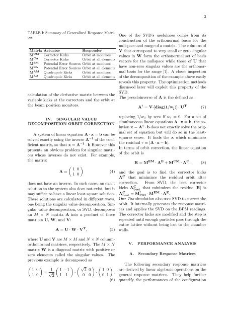
3 TABLE I: Summary of Generalized Response Matrices Matrix Actuator Responder M CM Corrector Kicks Orbit at monitors M CA Corrector Kicks Orbit at all elements M EM Potential Error Sources Orbit at monitors M EA Potential Error Sources Orbit at all elements M AM Quadrupole Kicks Orbit at monitors M AA Quadrupole Kicks Orbit at all elements calculation of the derivative matrix between the variable kicks at the correctors and the orbit at the beam position monitors. IV. SINGULAR VALUE DECOMPOSITION ORBIT CORRECTION A system of linear equation A · x = b can be solved exactly using the inverse A −1 of the coefficient matrix, so that x = A −1 · b However this presents an obvious problem for singular matrices whose inverses do not exist. For example, the matrix ( ) 1 0 A = (4) 1 0 does not have an inverse. In such cases, an exact solution to the system also does not exist, but it may suffice to have a linear least square solution. These solutions are calculated in different ways, one being the singular value decomposition. Singular value decomposition, or SVD, decomposes an M × N matrix A into a product of three matrices U, W, and V: A = U · W · V T , (5) where U and V are M × M and N × N columnorthonormal matrices, respectively. The M × N matrix W is a diagonal matrix with positive or zero elements called the singular values. The previous example is decomposed as ( ) 1 0 = 1 ( ) ( √ ) ( ) 1 −1 2 0 1 0 √ · · . 1 0 2 1 1 0 0 0 1 (6) One of the SVD’s usefulness comes from its construction of the orthonormal bases for the nullspace and range of a matrix. The columns of V that correspond to very small or zero singular values in W form the orthonormal set of basis vectors for the nullspace while those of U that have non-zero singular values are the orthonormal basis for the range [7]. A closer inspection of the decomposition of the example above easily reveals this property. The optimization methods discussed later will exploit this property of the SVD. The pseudoinverse of A is the defined as : A † = V·[diag(1/w j )] · U T (7) replacing 1/w j by zero if w j = 0. For a set of simultaneous linear equations A · x = b, the solution x = A † · b does not exactly solve the original set of equation but will do so in the leastsquares sense. It finds the x which minimizes the residual r ≡ |A · x − b|. In terms of orbit correction, the linear equation of the orbit is R = M EM · A E + M CM · A C , (8) and the goal is to find the corrector kicks A C that minimizes the residual orbit after correction. From SVD, the best corrector kicks A C best that minimizes the residue |R| is A C best = M† CM · MEM · A E . Our Tao simulation also uses SVD to correct the orbit. It internally generates the response matrices and applies the SVD on the BPM readings. The corrector kicks are modified and the step is repeated until enough particles pass through the entire lattice without being lost to the chamber walls. V. PERFORMANCE ANALYSIS A. Secondary Response Matrices The following secondary response matrices are derived by linear algebraic operations on the general response matrices. They help further quantify the performances of the configuration
Page 1: Analysis and Optimization of Singul
Page 5 and 6: 5 keep proper dimensions for matrix
Page 7 and 8: 7 vector indicates that the last mo
Page 9 and 10: 9 TABLE V: Minimizing Corrector Red

Analysis and Optimization of Singular Value Decomposition Orbit ...

Create successful ePaper yourself

Delete template?

Save as template?