Robot learning for ball bouncing

More documents

Recommendations

Info

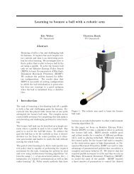
Manuscript under review by AISTATS 2012 the ball hits this plane next. This position then is desired to be the position, where the racket and the ball should collide. As for the hit positions, there might also be many different velocities of the ball, that could result from the hit and so the velocities have to be restricted, too. The desired velocitiy of the ball is chosen, such that the next collision of the ball with the racket lies in an area, where the end-effector has much degrees of freedom with corresponding buffers for all these. Ideally this would be somewhere in the middle of the space that can be reached by the end-effector easily. This desired point was set by a learning learning parameter(Θ 1 ) that set the y-value of the point with z given by the plane height and x = 0. To achieve a good resulting ball velocity that should have a low deviation to the desired ball velocity after the collision it is necessary to make sure that the paddle has an appropriate velocity and orientation, when it collides with the ball. This values also depend on the velocity the ball hits the paddle with. The orientation of the racket at the hit is chosen, such that both the velocity the ball hits the racket with and the desired velocity only possibly differ in normal direction of the paddle corresponding to reflection law assuming that the racket rests, i.e. has no zero velocity, and there is no damping etc... To compensate this velocity difference in normal direction and to take care of damping of unknown size the racket velocity in this direction is set to a value, such that the following chosen model equation holds for all these 1-dimensional velocities in racket normal direction: v ballout = v racket + d(v racket − v ballin ), (1) with d as damping. Thus it follows for the desired setting of the racket velocity: v racket = v ballout + dv ballin 1 + d (2) Since good values for d are a-priori not known, d here was choosen to be learning parameter(Θ 2 ) of this control method based on this given model. After the time and desired racket state at the next collision with the ball have been calculated, there has to be a movement of the racket that makes sure, that the racket has this desired state, when the ball hits the plane again. In order to avoid controlling difficulties this movement is desired to have a smooth trajectory with steady velocity, and to try to return to an basis point under the plane in somewhere in the movement, such that the racket has the possibility to accelerate to a desired velocity before it hits the ball. That means there are 3 given points of the trajectory, namely starting state, some intermediate basis state and the end state, where the racket should hit the ball. One possibility for such a smooth trajectory are linked polynomials, that are used in this approach. They were used by finding 2 polynomials, such that the first one goes from the current starting state through the intermediate basis state and the second from the intermediate basis state to the end state with the desired velocities. The polynomials also wer constraint to have equal velocities at the basis point, where they are connected. This desired velocity at the basis point was chosen such that it is directed to the desired collision point. The amount of the velocity was not fixed and instead used as settable learning parameter(Θ 3 ) together with the ratio of the time amounts of both trajectories(Θ 4 ), which have to sum up to the remaining time until the next collision. Furthermore it is much more convenient to represent this desired states of the racket not in the task space, but in the joint space and to define the trajectory there instead. One heavy advantage of doing so is that for controlling it is not necessary to call an inverse kinematics method all time to find the corresponding joint configuration for current task state given by the trajectory at this moment. Instead the inverse kinematics method is only called three times per step in order to get the joint states for the desired start point, the basis point and end points of the resulting trajectory. Since for both of the 2 linked trajectories it must hold that they start at some desired start point and end at some desired end point with desired velocities there are for each trajectory 4 constraints for each joint given by its angle and angle velocity at the beginning and at the end of the trajectory. Thus a polynomiala of degree 3 are sufficient to represent these one of both trajectories for each joint. Such polynomials have been used for this controlling method. 2.2 RDMPs - Rhythmic dynamic movement primitives To create complex movements for robots dynamic movement primitives, DMPs for short, have been shown to be quite versatile [SMI07]. With them it is possible to create complex non-linear trajectories which can be easily adapted to different goal positions and can be scaled with the time to create slower or faster movements. As the movement we need to be able to bounce the ball is an rhythmic one we use the rhythmic variation of the DMPs [SPNI04]. Rhythmic dynamic movement primitives or RDMPs for short
Manuscript under review by AISTATS 2012 consist of three equations. An transformation system, τż = α z (β z (g − y) − z), τẏ = z + f (3) where g is the setpoint of the oscillation of the rhythmic movement, α z and β z are time constants, τ is the temporal scaling factor to speed up or slow down the movement and y, ẏ are the desired position and velocity. The second equation is the canonical system, in this case an phase-amplitude oscillator, τṙ = α r (A − r), τ ˙φ = 1 (4) where r is the amplitude, A the desired amplitude and φ the phase of the oscillator. The last equation needed is the non-linear function f(r, φ) = N∑ ψ i ∗ wi T ∗ v i=1 v = [ r ∗ cos φ with (5) N∑ ψ i i=1 r ∗ sin φ ] T ψ i = exp((−h i (φ mod 2π) − c i ) 2 ) and where the w i are the weights which essentially describe the trajectory. So the learning parameters for these equations are the τ for the time scaling and the weights w i for the actual trajectory. For our setup we only use one RDMP and have therefore only one controllable DOF in the arm. The reason for this is so that we have fewer parameters which need to be learned and therefore an smaller learning space. 3 Learning methods Both approaches described in this paper need to be adapted to specific movements of the ball. For example an slow moving ball requires slower movements of the arm in comparison to an fast moving ball. This is especially true when the initial position and initial velocity of the ball is changing with each iteration of the simulation. This adaption is done through learning parameters which need to be automatically fitted to the task. For this comparison we are using the PoWER learning algorithm. 3.1 PoWER - Policy learning by Weighting Exploration with the Returns This learning algorithm is based on updating the learning parameters by doing multiple rollouts of the policy which should be learned with the same learning parameters each time disturbed by an small exploration value. The rewards for each of these rollouts will then be sorted and the X best rollouts will then be used to calculate the parameters for the next iteration of rollouts. This calculation is done by weighting the exploration values which were applied to the parameters for each rollout with the result of the Qsat and the Wst function and then multiplying it with its inverse but without the exploration values. The Qsat function takes the start state of the simulation, the action taken by the policy and the resulting ending state of the simulation as an input and uses this information to provide an evaluation on how good this action was given the states of the simulation. The Wst function is used to provide extra weight to certain states of the simulation making it possible to provide an boost for parameters of the policy which resulted in winning state or to punish when the last state of the simulation was especially bad. This algorithm is then run either until the parameters have converged to an optimum or until an maximum number of iterations is reached. We have chosen this method for learning the parameters as it performed best when compared to other learning methods such as eNAC and RWR [KP11]. It also treats the policy as an black box and does not need to know how it works or what it does at it operates entirely on the rewards and Qsat and Wst functions, making it perfectly suited to compare different policies against each other. But it cannot provide any guarantee that it will converge to the global maximum of the rewards and therefore not to the best possible values for the policy. Algorithm 1 PoWER - Policy learning by Weighting Exploration with the Returns Precondition: intial policy parameters Φ function PoWER(Φ) repeat for r ≤ mR do reward r = policy(Φ k + exploration r ) end for Φ k+1 = Φ k + until Φconverged return Φ optimal end function 4 Comparison mR ∑ Qsat t∗W st t∗exploration t t=1 mR ∑ Qsat t∗W st t t=1 We compare both approaches by providing them with the same initial state of the simulation. In this initial state the ball is placed directly above racket with zero velocity. We are also using the previously described PoWER learning algorithm to learn both policies in order to give them the same conditions. Initially we wanted to makes them easily comparable by using the same reward function for both approaches but as we
Page 1: Robot learning for ball bouncing De
Page 5: Manuscript under review by AISTATS

Robot learning for ball bouncing

Create successful ePaper yourself

Delete template?

Save as template?