
Create successful ePaper yourself
Turn your PDF publications into a flip-book with our unique Google optimized e-Paper software.
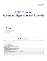
<strong>ENVI</strong> <strong>Tutorial</strong>:<br />
<strong>Working</strong> <strong>with</strong> <strong>NITF</strong> <strong>Data</strong><br />
Table of Contents<br />
OVERVIEW OF THIS TUTORIAL.....................................................................................................................................2<br />
Files Used in This <strong>Tutorial</strong> ..................................................................................................................................2<br />
EXERCISE #1: METADATA, TRES, DESES, CHIPPING, AND SAVING .......................................................................................2<br />
Viewing Metadata..............................................................................................................................................3<br />
Viewing a Text Segment ....................................................................................................................................3<br />
Tagged Record Extensions .................................................................................................................................3<br />
<strong>Data</strong> Extension Segments ..................................................................................................................................4<br />
Chipping the Image and Saving to <strong>NITF</strong> Format...................................................................................................6<br />
Examining the Output ..........................................................................................................................................................7<br />
Viewing the Output Metadata ...............................................................................................................................................7<br />
EXERCISE #2: RPC MAP INFORMATION .........................................................................................................................9<br />
Background on Replacement Sensor Models ........................................................................................................9<br />
RPCs...................................................................................................................................................................................9<br />
Viewing Map Information ...................................................................................................................................9<br />
EXERCISE #3: VIEWING COMPOSITE IMAGES AND EDITING PIA TRES.................................................................................. 11<br />
Saving to <strong>NITF</strong> Format..................................................................................................................................... 11<br />
Adding PIA TREs ............................................................................................................................................................... 11<br />
ENDING THE <strong>ENVI</strong> SESSION ..................................................................................................................................... 12
<strong>Tutorial</strong>: <strong>Working</strong> <strong>with</strong> <strong>NITF</strong> <strong>Data</strong><br />
Overview of This <strong>Tutorial</strong><br />
This tutorial introduces common tasks when working <strong>with</strong> National Imagery Transmission Format (<strong>NITF</strong>) files. The first<br />
exercise shows you how to open a <strong>NITF</strong> 2.1 multiple image segment file; how to view metadata, Tagged Record<br />
Extensions (TREs), and <strong>Data</strong> Extension Segments (DESes); how to chip (subset) the file; and how to save the chip to<br />
<strong>NITF</strong> format. The second exercise demonstrates the use of rapid positioning coordinate (RPC) map information in<br />
georeferencing a <strong>NITF</strong> file. The third exercise explains how to work <strong>with</strong> composite images and how to edit Profile for<br />
Imagery Access (PIA) TREs.<br />
Files Used in This <strong>Tutorial</strong><br />
<strong>ENVI</strong> Resource DVD: envidata\nitf<br />
File<br />
Description<br />
digitalglobe_ncdrd_chip.ntf <strong>NITF</strong> 2.1 Quickbird image of St. Petersburg, Russia<br />
target_example.ntf<br />
<strong>NITF</strong> 2.1 composite image<br />
The Quickbird file digitalglobe_ncdrd_chip.ntf is courtesy of Digital Globe and may not be reproduced <strong>with</strong>out<br />
explicit permission from Digital Globe. The file target_example.nitf was provided by the Joint Interoperability Test<br />
Command (JITC) for test purposes.<br />
Exercise #1: Metadata, TREs, DESes, Chipping, and Saving<br />
In this exercise, you will open a <strong>NITF</strong> 2.1 file; view metadata, TREs, and DESes; chip (subset) the file; and save multiple<br />
image segments to <strong>NITF</strong> format.<br />
1. From the <strong>ENVI</strong> main menu bar, select File → Open Image File. The Enter <strong>Data</strong> Filenames dialog appears.<br />
2. Navigate to envidata\nitf, select the file digitalglobe_ncdrd_chip.ntf, and click Open. The file<br />
appears in the Available Bands List as two image segments. Image segment #1 is a QuickBird image of St.<br />
Petersburg, Russia, and image segment #2 is an NCDRD cloud image.<br />
3. In the Available Bands List, right-click on the filename digitalglobe_ncdrd_chip.ntf, and select Load<br />
True Color. An RGB version of image segment #1 is loaded into a new display group.<br />
Leningrad<br />
Zoo<br />
Artillery museum<br />
Peter and Paul Fortress<br />
Figure 1: Overview of St. Petersburg <strong>NITF</strong> Image<br />
2<br />
<strong>ENVI</strong> <strong>Tutorial</strong>: <strong>Working</strong> <strong>with</strong> <strong>NITF</strong> <strong>Data</strong>
<strong>Tutorial</strong>: <strong>Working</strong> <strong>with</strong> <strong>NITF</strong> <strong>Data</strong><br />
Viewing Metadata<br />
1. In the Available Bands List, right-click on the filename digitalglobe_ncdrd_chip.ntf and select View<br />
<strong>NITF</strong> Metadata. The <strong>NITF</strong> Metadata Viewer dialog appears. The metadata for this file is organized into separate<br />
entries for the file header, image segments, a text segment, and <strong>Data</strong> Extension Segments (DESes). The<br />
metadata fields are described in more detail in the following specification document:<br />
http://www.ismc.nga.mil/ntb/baseline/docs/2500a/index.html<br />
2. In the <strong>NITF</strong> Metadata Viewer, click the + symbol next to <strong>NITF</strong> file header to see metadata describing the file<br />
properties.<br />
3. Click the + symbol next to Image segment #1 and Image segment #2 to see metadata describing the<br />
image characteristics. Image segments contain raster image data, intended for display or analysis. Under image<br />
segment #2, notice that the Image Representation field contains the value “NODISPLY.” This means the image<br />
segment will not be chipped if you save it to <strong>NITF</strong> format.<br />
Viewing a Text Segment<br />
This file contains a text segment, which consists of textual information not intended for graphical display. Most of the<br />
time, text segments are provided to supplement the graphic content in the dataset.<br />
1. In the <strong>NITF</strong> metadata viewer, click the + symbol next to Text segment #1.<br />
2. Click on the line that says Text: . A Text dialog appears <strong>with</strong> the information contained <strong>with</strong>in<br />
the text segment subheader. In this case, the text segment contains the end-user license agreement from Digital<br />
Globe.<br />
3. Close the Text dialog.<br />
Tagged Record Extensions<br />
When you click the + symbols to expand the file header, image segments, and DESes in the <strong>NITF</strong> Metadata Viewer, you<br />
will notice various colored icons that say “TRE.” These are tagged record extensions, which contain information about the<br />
segment they are in. The file header can contain one or more TREs that apply to the entire data set, and each segment<br />
(image, text, annotation) can also have one or more TREs associated <strong>with</strong> it. TREs can specify attributes such as<br />
processing history, information about specific targets in an image, collection information, and other types of metadata.<br />
A white TRE icon contains metadata for a TRE that you cannot edit when saving the file. A green icon contains metadata<br />
that you can edit when saving the file.<br />
Each TRE supported by the <strong>NITF</strong>/NSIF Module references an XML definition file that is installed <strong>with</strong> your <strong>ENVI</strong> software if<br />
you purchased the <strong>NITF</strong>/NSIF Module. For a full list of supported TREs and links to their specifications, see Appendix A of<br />
the <strong>NITF</strong>/NSIF User’s Guide (available as a PDF file from the ITT Visual Information Solutions website or included <strong>with</strong><br />
your <strong>NITF</strong>/NSIF Module installation).<br />
Figure 2: TREs for Image Segment #1<br />
3<br />
<strong>ENVI</strong> <strong>Tutorial</strong>: <strong>Working</strong> <strong>with</strong> <strong>NITF</strong> <strong>Data</strong>
<strong>Tutorial</strong>: <strong>Working</strong> <strong>with</strong> <strong>NITF</strong> <strong>Data</strong><br />
When working <strong>with</strong> <strong>NITF</strong> data outside of this tutorial, your data may contain some TREs that do not have an associated<br />
XML file. These TREs are displayed <strong>with</strong> a “Definition Unknown” label next to their name. Their contents may be viewable<br />
if the TREs do not contain binary data. <strong>ENVI</strong> will save these TREs.<br />
<strong>Data</strong> Extension Segments<br />
In the <strong>NITF</strong> Metadata Viewer, you will also see two blue icons that say “DES.” These are data extension segments, which<br />
are similar to TREs because they contain information that cannot be stored in other <strong>NITF</strong> segments.<br />
The file you are working <strong>with</strong> is a <strong>NITF</strong> 2.1 Commercial <strong>Data</strong>set Requirements Document (NCDRD) file that contains two<br />
shapefile DESes indicated by the word “CSSHPA.”<br />
1. Click on the + symbol next to DES #1: CSSHPA DES to view its metadata. Then click the + symbol next to<br />
User Defined Subheaders. You will see that this is a CLOUD_SHAPES DES, which is a polygon shapefile<br />
containing cloud locations.<br />
Figure 3: Example CLOUD_SHAPES DES<br />
2. In the <strong>NITF</strong> Metadata Viewer, click Load DES Shapefiles. This button is only available when you open NCDRD<br />
files <strong>with</strong> at least one CSSHPA DES. <strong>ENVI</strong> extracts the corresponding shapefile element, coverts it to <strong>ENVI</strong> vector<br />
format (EVF), and loads into the Available Vectors List.<br />
3. In the Available Vectors List, select the layer named digitalglobe_ncdrd_chip_CLOUD_SHAPES, and click<br />
Load Selected. The Load Vectors dialog appears.<br />
4. Select Display #1, and click OK. Polygon vectors overlay the image segment in the display group, roughly<br />
outlinining the boundaries of clouds. The Vector Parameters dialog also appears.<br />
4<br />
<strong>ENVI</strong> <strong>Tutorial</strong>: <strong>Working</strong> <strong>with</strong> <strong>NITF</strong> <strong>Data</strong>
<strong>Tutorial</strong>: <strong>Working</strong> <strong>with</strong> <strong>NITF</strong> <strong>Data</strong><br />
Cloud shapefiles<br />
Figure 4: Vectors roughly outlining cloud boundaries<br />
5. Use the Vector Parameters dialog to change the color of the vector layer to another color.<br />
6. In the <strong>NITF</strong> Metadata Viewer, click on the + symbol next to DES #2: CSSHPA DES to view its metadata. Then<br />
click the + symbol next to User Defined Subheaders. You will see that this is an IMAGE_SHAPE DES, which is<br />
a single-polygon shapefile defining the original image extent.<br />
Figure 5: Example IMAGE_SHAPE DES<br />
5<br />
<strong>ENVI</strong> <strong>Tutorial</strong>: <strong>Working</strong> <strong>with</strong> <strong>NITF</strong> <strong>Data</strong>
<strong>Tutorial</strong>: <strong>Working</strong> <strong>with</strong> <strong>NITF</strong> <strong>Data</strong><br />
7. When you are finished, close the Available Vectors List, Vector Parameters, and <strong>NITF</strong> Metadata Viewer dialogs.<br />
The vector shapefiles disappear from the display group. (If you want to view them again in the future, you can<br />
select Vector → Available Vectors List from the <strong>ENVI</strong> main menu bar, then load the desired vectors to the<br />
display group.)<br />
Chipping the Image and Saving to <strong>NITF</strong> Format<br />
In these steps, you will attempt to chip (subset) both image segments and output them to <strong>NITF</strong> format.<br />
1. From the <strong>ENVI</strong> main menu bar, select File → Save File As → <strong>NITF</strong>. The Select <strong>NITF</strong> Output File dialog appears.<br />
The left side of the dialog lists both image segments associated <strong>with</strong> the file.<br />
2. Select the image segment named digitalglobe_ncdrd_chip.ntf M1043BFF00. Information about the file<br />
is displayed, along <strong>with</strong> Spatial Subset and Spectral Subset buttons and an All Image Segments check box.<br />
3. Click to enable the All Image Segments check box to select both image segments for saving. Special rules<br />
apply when saving any <strong>NITF</strong> image <strong>with</strong> multiple image segments:<br />
You can save one or all of the image segments to an output <strong>NITF</strong> file. If you have three or more image<br />
segments, you cannot use Ctrl-click to select multiple image segments. If you hold down the Shift key<br />
and select another segment, the last segment you selected is highlighted (not all segments).<br />
You cannot create a <strong>NITF</strong> file <strong>with</strong> multiple image segments if the input file does not contain multiple<br />
image segments.<br />
The Spectral Subset button is not available if all segments are selected.<br />
If you select all image segments and uncheck All Image Segments, the previously selected image<br />
segment is selected.<br />
You can edit multiple image segment metadata the same was as single-image output.<br />
You cannot save image segments containing masks to an output <strong>NITF</strong> file.<br />
You cannot change the <strong>NITF</strong> file version or compression parameters when saving multiple image<br />
segments.<br />
4. Click Spatial Subset. The Select Spatial Subset dialog appears.<br />
5. Click Image. The Subset by Image dialog appears.<br />
6. Leave the Samples and Lines values at 400, and move the red box to any location <strong>with</strong>in the image. Click OK.<br />
7. Click OK on the Select Spatial Subset dialog and the Select <strong>NITF</strong> Output File dialog. The <strong>NITF</strong> Output Parameters<br />
dialog appears.<br />
8. Select an output filename and click OK. After processing is complete, the output file (and its associated image<br />
segments) are added to the Available Bands List.<br />
6<br />
<strong>ENVI</strong> <strong>Tutorial</strong>: <strong>Working</strong> <strong>with</strong> <strong>NITF</strong> <strong>Data</strong>
<strong>Tutorial</strong>: <strong>Working</strong> <strong>with</strong> <strong>NITF</strong> <strong>Data</strong><br />
Figure 6: <strong>NITF</strong> Output Parameters dialog<br />
Examining the Output<br />
9. In the Available Bands List, right-click on Image Segment #2 of your chipped image and select Load Band to<br />
New Display. Note that image segment #2 (the NCDRD cloud image) was not chipped upon output because the<br />
Image Representation metadata value was “NODISPLY” (in the original image).<br />
10. Close Display #2 (containing Image Segment #2).<br />
11. In the Available Bands List, right-click on the new filename and click Load True Color to . In the next<br />
step, you will use <strong>ENVI</strong>’s Dynamic Overlay feature to compare the original (unchipped) image in Display #1 to the<br />
chipped image in Display #2.<br />
12. From any display group menu bar, select Tools → Link → Link Displays. The Link Displays dialog appears.<br />
13. Ensure that the Display #1 and Display #2 toggle buttons are both set to Yes. Also ensure the Dynamic<br />
Overlay toggle button is set to On. Click OK.<br />
14. Click in one of the Image windows to toggle between the original (unchipped) image and the chipped image.<br />
Notice the color differences between the two images. <strong>ENVI</strong> automatically assigned a default 2% linear stretch to<br />
the unchipped image, but not to the chipped image that you saved.<br />
Viewing the Output Metadata<br />
15. In the Available Bands List, right-click on the new filename, and select View <strong>NITF</strong> Metadata. The <strong>NITF</strong><br />
Metadata Viewer dialog appears.<br />
16. Browse through the metadata and notice that the <strong>NITF</strong>/NSIF Module retained the input metadata, TREs, and<br />
DESes. An exception is that some fields in the image and file header metadata were updated to indicate<br />
processing changes to the file upon chipping. Also notice that an ICHIPB TRE was added to Image Segment #1,<br />
which indicates the image was chipped.<br />
If you click the + symbol to expand the <strong>NITF</strong> file header metadata, you will see the Originating Station ID,<br />
Originator’s Name, and Originator’s Phone fields were changed to the defaults set in the <strong>NITF</strong> configuration file.<br />
On Windows, the <strong>NITF</strong> configuration file is located at<br />
C:\Program Files\ITT\IDLxx\products\envixx\menu\nitf.cfg.<br />
7<br />
<strong>ENVI</strong> <strong>Tutorial</strong>: <strong>Working</strong> <strong>with</strong> <strong>NITF</strong> <strong>Data</strong>
<strong>Tutorial</strong>: <strong>Working</strong> <strong>with</strong> <strong>NITF</strong> <strong>Data</strong><br />
On Unix, the file is located in /usr/local/itt/idlxx/products/envixx/menu/nitf.cfg.<br />
To learn more about changing the default values for these (and other) fields in the <strong>NITF</strong> configuration file, see<br />
“The <strong>NITF</strong> Configuration File” in <strong>ENVI</strong> Help.<br />
17. Click Load DES Shapefiles.<br />
18. In the Available Vectors List, select the CLOUD_SHAPES layer corresponding to the output file you created.<br />
Click Load Selected. The Load Vectors dialog appears.<br />
19. Select New Vector Window, and click OK. Note the full extent of the DES shapefile. It was not chipped upon<br />
output.<br />
20. When you are finished, close all dialogs and display groups except for the Available Bands List and <strong>NITF</strong> Metadata<br />
Viewer. You will use the same data file for the next exercise.<br />
8<br />
<strong>ENVI</strong> <strong>Tutorial</strong>: <strong>Working</strong> <strong>with</strong> <strong>NITF</strong> <strong>Data</strong>
Exercise #2: RPC Map Information<br />
<strong>Tutorial</strong>: <strong>Working</strong> <strong>with</strong> <strong>NITF</strong> <strong>Data</strong><br />
In this exercise, you will learn how the <strong>NITF</strong>/NSIF Module uses RPC map information to georeference a file. You will open<br />
the digitalglobe_ncdrd_chip.ntf file (which contains RPC map information) and view the map information used<br />
for georeferencing.<br />
The <strong>NITF</strong>/NSIF Module uses a variety of different map information for georeferencing:<br />
Replacement sensor model (RSM) TREs<br />
Rapid positioning capability (RPC) TREs<br />
DIGEST GeoSDE TREs (MAPLOB, PRJPSB, and GEOPSB TREs)<br />
IGEOLO image header field<br />
If a <strong>NITF</strong> file contains RPC or RSM map information, the <strong>NITF</strong>/NSIF Module in <strong>ENVI</strong> uses that information to georeference<br />
the file. If a file does not contain RPCs or RSMs, <strong>ENVI</strong> looks for the items in the above list (in that order) to georeference<br />
the file. This exercise focuses on the use of RPCs only.<br />
For a full discussion on how <strong>ENVI</strong> uses non-standard projections such as affine map transformations, RPCs, and RSMs,<br />
see “Non-Standard Projections” in <strong>ENVI</strong> Help.<br />
Background on Sensor Models<br />
Sensor models are a type of map information used to define the physical relationship between image coordinates and<br />
ground coordinates. A sensor model is a mathematical model that replaces the rigorous (physical) sensor model<br />
associated <strong>with</strong> a specific sensor by representing the model’s ground-to-image relationship. It is used to map a 3D ground<br />
point to a 2D image point. Various commercial spaceborne image providers utilize replacement sensor models, particularly<br />
RPCs, which are one type. Two sensor models that <strong>ENVI</strong> uses are RPCs and RSMs. This tutorial only discusses the use of<br />
RPCs.<br />
RPCs<br />
Rational polynomial coefficients (RPCs) are one type of sensor model. RPCs are not the same as a map projection; rather,<br />
they model the ground-to-image relationship as a third-order, rational, ground-to-image polynomial. You can use RPCs to<br />
perform orthorectification and DEM extraction in <strong>ENVI</strong>.<br />
Quickbird data include pre-computed RPCs <strong>with</strong> the imagery. If your file has RPC information, you can automatically<br />
derive RPC-based geolocation information for individual pixels in an image. This method is not as geographically accurate<br />
as performing a full orthorectification, but it is less computationally and disk-space intensive.<br />
If your image file has pre-computed RPC information, <strong>ENVI</strong> uses the mean elevation value used in the RPC transformation<br />
for the entire image. However, you can significantly increase the geolocation accuracy of the image if you associate the<br />
image <strong>with</strong> a DEM.<br />
The <strong>NITF</strong>/NSIF Module reads RPC information from a <strong>NITF</strong> file and creates an RPC00A or RPC00B TRE. If either of these<br />
TREs exists in a <strong>NITF</strong> file, <strong>ENVI</strong> uses the RPC model to emulate a projection by default. The projection description<br />
includes the string *RPC* prior to the name of the coordinate system in which the image resides.<br />
Viewing Map Information<br />
1. In the <strong>NITF</strong> Metadata Viewer dialog, click the + symbol next to Image segment #1<br />
(digitalglobe_ncdrd_chip.ntf) to expand its contents.<br />
2. Scroll until you see the RPC00B TRE. Click the + symbol next to this TRE to expand its contents. All of the<br />
information here was derived from the RPC map information provided <strong>with</strong> the Quickbird image of St. Petersburg.<br />
<strong>ENVI</strong> read this information into an RPC00B TRE and georeferenced the file using the coefficients shown here.<br />
3. Click Cancel in the <strong>NITF</strong> Metadata Viewer dialog.<br />
9<br />
<strong>ENVI</strong> <strong>Tutorial</strong>: <strong>Working</strong> <strong>with</strong> <strong>NITF</strong> <strong>Data</strong>
<strong>Tutorial</strong>: <strong>Working</strong> <strong>with</strong> <strong>NITF</strong> <strong>Data</strong><br />
4. In the Available Bands List, you should see a Map Information icon under<br />
digitalglobe_ncdrd_chip.ntf. This indicates that the file is georeferenced. Click the + symbol to expand<br />
its contents. The Proj field shows that RPCs are used to emulate a Geographic Lat/Lon projection.<br />
Figure 7: Map Info icon showing RPC map information<br />
5. In the Available Bands List, right-click on digitalglobe_ncdrd_chip.ntf, and select Load True Color.<br />
6. Double-click in the Image window to display the Cursor Location/Value tool.<br />
7. Move around the image and note how <strong>ENVI</strong> displays geographic latitude and longitude coordinates. Also note<br />
that the Cursor Location/Value tool shows the Projection as *RPC* Geographic Lat/Lon.<br />
8. When you are finished, select File → Close All Files from the <strong>ENVI</strong> main menu bar, then click Yes to close all<br />
files.<br />
10<br />
<strong>ENVI</strong> <strong>Tutorial</strong>: <strong>Working</strong> <strong>with</strong> <strong>NITF</strong> <strong>Data</strong>
<strong>Tutorial</strong>: <strong>Working</strong> <strong>with</strong> <strong>NITF</strong> <strong>Data</strong><br />
Exercise #3: Viewing Composite Images and Editing PIA TREs<br />
In this exercise, you will learn about composite images and how to edit Profile for Imagery Access (PIA) TREs when<br />
saving a <strong>NITF</strong> file.<br />
1. From the <strong>ENVI</strong> main menu bar, select File → Open Image File. The Enter <strong>Data</strong> Filenames dialog appears.<br />
2. Navigate to envidata\nitf, select the file target_example.ntf, and click Open. This is a composite image<br />
consisting of two image segments and various annotation segments. The first entry that appears in the Available<br />
Bands List is the RGB composite image. The next two entries are the image segments that make up the<br />
composite image.<br />
3. Click Load RGB. The composite image is loaded to a new display group.<br />
4. In the Available Bands List, right-click on Image Segment #1 and select Load Band to New Display. The<br />
first image segment appears in a new display group.<br />
5. Double-click inside the Image Window in Display #1 (composite image). The Cursor Location/Value dialog<br />
displays. Move your cursor around the composite image, then around the corresponding image segment (for the<br />
same location). Note that the composite image does not display geographic information, but the image segment<br />
does. The composite image is simply a graphical depiction of the individual image and annotation segments, but<br />
it does not provide map information.<br />
Saving to <strong>NITF</strong> Format<br />
1. From the <strong>ENVI</strong> main menu bar, select File → Save File As → <strong>NITF</strong>. The Select <strong>NITF</strong> Output File dialog appears.<br />
2. Select the COMPOSITE image for output. Notice that all of the image segments are selected for output when<br />
you select the composite image. The All Image Segments check box is also automatically checked.<br />
3. Click OK. The <strong>NITF</strong> Output Parameters dialog appears.<br />
4. Click Edit <strong>NITF</strong> Metadata. The <strong>NITF</strong> Metadata Editor dialog appears.<br />
Adding PIA TREs<br />
The <strong>NITF</strong> Metadata Editor lets you add or delete Profile for Imagery Access and Profile for Imagery Archive (PIA) TREs,<br />
which hold information required by the Standards Profile for Imagery Access (SPIA). A variety of government agencies<br />
require these TREs in <strong>NITF</strong> image products. In this step, you will simulate adding a Profile for Imagery Access Target<br />
Descriptive (PIATGB) TRE to mark a target of interest in the data.<br />
1. In the <strong>NITF</strong> Metadata Editor, select Image segment #1 and click Add PIA Tags. The Add PIA Tags dialog<br />
appears.<br />
2. Change the value for PIATGB (PIA Target Tag) to 1.<br />
3. Click OK. The metadata under Image segment #1 expands in the <strong>NITF</strong> Metadata Editor. A new green TRE<br />
symbol appears at the bottom of the metadata.<br />
4. Click the + symbol to expand the new TRE.<br />
11<br />
<strong>ENVI</strong> <strong>Tutorial</strong>: <strong>Working</strong> <strong>with</strong> <strong>NITF</strong> <strong>Data</strong>
<strong>Tutorial</strong>: <strong>Working</strong> <strong>with</strong> <strong>NITF</strong> <strong>Data</strong><br />
5. Double-click on any of the empty fields such as Target UTM. A text entry dialog appears.<br />
6. Enter your own text and click OK. A text entry dialog for the next PIATGB TRE metadata field appears.<br />
7. Continue adding your own values for the PIATGB TRE metadata in this manner.<br />
8. Click OK in the <strong>NITF</strong> Metadata Editor. <strong>ENVI</strong> validates your entry and issues an error message if you entered<br />
incorrect data.<br />
9. In the <strong>NITF</strong> Output Parameters dialog, enter an output filename, and click OK.<br />
10. When the output file appears in the Available Bands List, right-click on its filename and select View <strong>NITF</strong><br />
Metadata.<br />
11. Examine the metadata in the output file. You should see the new PIATGB TRE metadata.<br />
Ending the <strong>ENVI</strong> Session<br />
When you are finished, close all dialogs and select File → Close All Files from the <strong>ENVI</strong> main menu bar.<br />
12<br />
<strong>ENVI</strong> <strong>Tutorial</strong>: <strong>Working</strong> <strong>with</strong> <strong>NITF</strong> <strong>Data</strong>