Comparison of Transfer Matrix (T-matrix) and Coupling of ... - Infoteh

INFOTEH-JAHORINA Vol. 12, March 2013.
Comparison of Transfer Matrix (T-matrix) and
Coupling of Modes in Time (CMT) Models of
Coupled Microring Resonator Filters
Miljan Dašić
Student of the first level studies
Faculty of Electrical Engineering, University of Belgrade,
Belgrade, Serbia
miljandasic@yahoo.com
Abstract—The aim of this paper is to use theoretical
models of coupled microring resonator filter to show its
operation and to apply those calculations in order to
maximize drop port power. Coupled microring resonators are
one of fundamental elements in photonic devices. They have
good resonator characteristics useful for filter applications,
because arbitrary -3dB bandwidth and FSR(Free Spectral
Range) are easily designed. Theoretical models include T-
matrix (Transfer Matrix) and CMT (Coupling of Modes in
Time). A comparison of those models is shown. CMT model is
applied in optimization of transmission to the drop port.
coupling coefficient of k i
, while the other linear system
represents coupling of the second bus to the ring with
Key words-model; transfer matrix; coupling of modes in
time; microring; resonator; filters;
I. INTRODUCTION
INTEGRATED silicon based photonics has many
promising applications in optical telecommunications,
optoelectronics and optical signal processing [1]–[4]. The
integration of silicon photonics and electronic circuits
offers the prospect of low energy devices, circuits and
systems for applications including on-chip and processorto-memory
interconnects [3], [4], as well as photonic
analog-to-digital converters [5]. Other applications include
nonlinear and quantum devices for applications in quantum
information and computing [6]. An important photonic
device, and one of the earliest concepts realized in
integrated photonics, is the resonant channel add-drop
filter. Microring resonators are particularly well suited for
add-drop filter applications [7], [8] because of their
traveling wave structure that allows for a natural separation
of the four ports (in, through, drop, add).
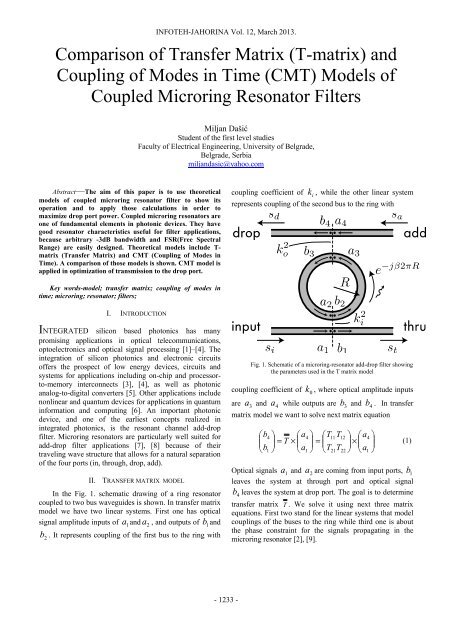
II. TRANSFER MATRIX MODEL
In the Fig. 1. schematic drawing of a ring resonator
coupled to two bus waveguides is shown. In transfer matrix
model we have two linear systems. First one has optical
signal amplitude inputs of a1
and a 2
, and outputs of b1
and
b
2
. It represents coupling of the first bus to the ring with
Fig. 1. Schematic of a microring-resonator add-drop filter showing
the parameters used in the T matrix model
coupling coefficient of k
0
, where optical amplitude inputs
are a
3
and a
4
while outputs are b
3
and b
4
. In transfer
matrix model we want to solve next matrix equation
⎛b
⎜
⎝b
4
1
⎞ ⎛a
⎟ = T ×
⎜
⎠ ⎝a
4
1
⎞ ⎛T
⎟ =
⎜
⎠ ⎝T
11
21
T
T
12
22
⎞ ⎛
× a
⎟
⎜
⎠ ⎝a
Optical signals a
1
and a2
are coming from input ports, b
1
leaves the system at through port and optical signal
b4
leaves the system at drop port. The goal is to determine
transfer matrix T . We solve it using next three matrix
equations. First two stand for the linear systems that model
couplings of the buses to the ring while third one is about
the phase constraint for the signals propagating in the
microring resonator [2], [9].
4
1
⎞
⎟
⎠
(1)
- 1233 -

⎛b
⎛ − − ⎞
1 ⎞ ⎛a
⎞ 1 k
1 ⎜
i
j ki
⎟ ⎛a1
⎞
⎜
⎟ = t ×
⎜
⎟ =
×
⎜
⎟
⎝b
⎠ ⎝ ⎠
⎜ − ⎟
2
a2
⎝−
j k 1 k ⎠ ⎝a
i i 2 ⎠
(2)
⎛b
⎛ − − ⎞
3 ⎞ ⎛a
⎞ 1 k
3 ⎜
o
j ko
⎟ ⎛a3
⎞
⎜
⎟ = τ ×
⎜
⎟ =
×
⎜
⎟
⎝b
⎠ ⎝ ⎠
⎜ − ⎟
4
a4
⎝−
j k 1 k ⎠ ⎝a
o o 4 ⎠
(3)
⎛a
⎜
⎝a
2
− jβπR
⎞ ⎛e
⎞ ⎛b
⎟ = ⎜ ⎟
×
⎜
− jβπR
⎠ ⎝0 e ⎠ ⎝b
3
0
In Eq. 4 j is imaginary one, βπR
is the product of
propagation constant and half of the circumference of the
ring and term R is inner radius of the ring. The expression
for beta is
2π
β n ×
(5)
= g
where n is group refractive index. We use notation:
g
λ
⎛t11
t12
⎞
t =
⎜
⎟
⎝t21t22
⎠
⎛τ11τ12
⎞
τ =
⎜
⎟
⎝τ
21τ
22 ⎠
When matrix equations are written in developed form, we
obtain
b = t
b
b
b
1
2
3
4
11
= t
21
11
21
1
1
= τ a
3
= τ a
a + t
3
12
a + t
22
a
12
22
2
a
2
+ τ a
4
+ τ a
Together with the phase constraints
a
a
3
2
= b × e
2
= b × e
3
− jβπR
− jβπR
The algorithm is to solve Eq. 7.4 for a3
and to obtain b2
in
terms of a4
and b4
using Eq. 8.1. Then plug in a 3
to Eq.
7.3 which leads to an expression of b 3
in terms of
( a
4
, b
4
). We were using Eq. 8.1, Eq. 7.3 and Eq. 7.4. In
similar way using Eq. 8.2, Eq. 7.1 and Eq. 7.2 we solve
a2
and b2
in terms of ( a
1
, b
1
). Then we have to combine
expressions obtained by this separate solvings using
4
2
3
⎞
⎟
⎠
(4)
(6)
(7)
(8)
constraint equations (Eq. 8.1 and Eq. 8.2) which leads to
this solution
b
4
1
= T
11
b = T a
21
a
4
4
+ T
+ T
like in Eq. 1, where expressions for transfer matrix
elements are
T
11
T
22
τ
=
22
T
T
t
=
12
21
11
− j 2βπR
+ e t
−
(1 − e
22
j 2
12
22
a
a
1
1
( τ12τ
21
−τ11τ
22
)
βπR
τ t )
11 22
− jβπR
e τ
21t21
=
− j 2βπR
( 1−
e τ11t22)
− jβπR
e t12τ
12
=
− j2βπR
( 1−
e τ11t22)
− j 2βπR
+ e τ11(
t12t21
− t
− j 2βπR
(1 − e τ t )
11 22
t
11 22
)
(9)
(10)
Here T12
represents normalized drop port power and T 22
represents normalized through port power. Now we apply
those expressions from Eq. 10 to calculate spectral
response of a filter made of two bus waveguides that are
coupled to the microring-resonator. We have chosen free
spectral range of 2 THz and -3dB bandwidth of 40 GHz. It
is known that free spectral range of a microring-resonator
is determined by ring’s radius [2].
c
c
FSR = ⇒ R =
(11)
2πRn
2πn
FSR
g
Taking the Eq. 12 from reference [1] and using
c c
λ = ⇒ dλ
=
2
f f
df (12)
gives us the relation for -3dB bandwidth
2
π ⋅ Δf dB
= k 2FSR
(13)
−3 ⋅
Therefore we define normalized coupling
× Δf −3dB
ξ = π
(14)
2FSR
Delay in group time is calculated using this formula
1 dΦ
t g
= −
2π df
where Φ is the phase and f is the frequency.
g
(15)
- 1234 -

Symmetric coupling
k
i
= k o
= ξ
Assymetric coupling
k
i
=
o
2 ξ,
k = 3ξ
Amplitude of T-matrix complex elements
1
0.9
0.8
0.7
0.6
0.5
0.4
0.3
0.2
Transfer matrix method
T11
T21
T12
T22
Amplitude of T-matrix complex elements
1
0.9
0.8
0.7
0.6
0.5
0.4
0.3
0.2
Transfer matrix method
T11
T21
T12
T22
0.1
0.1
Phase of T-matrix complex elements (rad)
0
193 194 195 196 197 198 199
f (THz)
20
15
10
5
0
(a)
Phases of transfer matrix complex elements
T11
T21
T12
T22
Phase of T-matrix complex elements (rad)
0
193 194 195 196 197 198 199
f (THz)
20
15
10
5
0
(a)
Phases of transfer matrix complex elements
T11
T21
T12
T22
Group time delay (ps)
-5
193 194 195 196 197 198 199
f (THz)
4
3
2
1
0
-1
(b)
Delay in group time
T11
T12
T21
T22
Group time delay (ps)
-5
193 194 195 196 197 198 199
f (THz)
4
3
2
1
0
-1
(b)
Delay in group time
T11
T12
T21
T22
-2
-2
-3
193 194 195 196 197 198 199
f (THz)
(c)
Fig. 2. Frequency spectra of T-matrix elements’
amplitude, phase and group time delay - (a), (b), (c)
-3
193 194 195 196 197 198 199
f (THz)
(c)
Fig. 3. Frequency spectra of T-matrix elements’
amplitude, phase and group time delay - (a), (b), (c)
- 1235 -

In Fig. 2 and Fig. 3 frequency spectra of T-matrix
elements’ amplitude, phase and group time delay are given,
in symmetric and chosen asymmetric case, respectively.
We can notice that symmetric coupling affords 100%
transmission to the drop port. In the phase and group time
delay plots we can notice differentiation of the bus lines,
caused by the asymmetric coupling.
III. COUPLING OF MODES IN TIME (CMT) MODEL
Coupled-mode theory in time (CMT) provides a
simple model that affords all necessary physics of the
resonant add-drop filter problem, including resonance, loss
and coupling to input and output ports [1,2,6]. The system
of equations that describes a single-resonator filter excited
by a monochromatic input wave at angular frequency ω is
d
dt
a t)
= jωa(
t)
= ( jω
− r)
a(
t)
− j
(
0
s ( t)
= s ( t)
− j
t
s ( t)
= − j
d
i
2r
d
2r
a(
t)
e
a(
t)
2r
s ( t)
e
i
(16)
where a(t) is energy amplitude of the ring resonant mode,
s i , s t , s d , are the power-normalized amplitudes of input,
through and drop port waves [2]. With input wave s i
incident, some excitation is picked up by the resonator, and
the remaining field interferes with that leaving the
resonator in the through port and is carried away by
through-port wave s t . The energy stored in the resonator is
|a(t)| 2 and according to Eqs. (16) the energy amplitude a(t)
decays at a total rate r, comprising decay rates describing
external coupling to the input port, r e , to the drop port, r d ,
and to loss mechanisms, r o :
r = r e
+ r d
+ r o
(17)
The coupling rates r e and r d are determined in the
evanescent-coupling geometry in Fig. 8 by the size of the
ring-waveguide coupling gaps [1,9]. The decay rates are
related to decay time constants as r i = 1/τ I , for i = {e,d,o}.
Since τ is a field time constant, the associated photon
lifetime of the resonant cavity (which measures decay of
intensity) is τ/2.
The through-port and drop-port responses of the device
can be found from Eqs. (16) as
2
s t
= (ω −ω 0 )2 + (r 0
+ r d
− r e
) 2
(18)
s i
(ω −ω 0
) 2 + (r 0
+ r d
+ r e
) 2
2
s d
=
s i
4r e
r d
(19)
( ω −ω 0 ) 2 + r 2
The drop-port response is Lorentzian, with a full 3dB
bandwidth Δω 3dB = 2r.
Unlike a full scattering model (T matrix model) using
transfer matrices, the CMT model addresses only one
resonant mode of the ring and does not include geometry
information that can define a free spectral range (FSR).
Resonant frequencies are determined by the resonant
condition
f
m
c
= m
(20)
2πRn
where c is the speed of light in vacuum, R is the ring
resonator radius, and n eff is the (frequency dependent)
effective index of the guided mode. The FSR is given by
c
Δf FSR
=
(21)
2π Rn g
where n
g
is group effective index of the guided mode.
Fig. 4. Schematic of a single microring-resonator add-drop filter showing
the parameters used in the CMT model.
IV. CORRESPONDENCE OF CMT AND T-MATRIX
MODELS
We have derived T-matrix and CMT models of
coupled microring resonator filters. Now we will compare
those models. In Fig. 5 we show wavelength spectra of
amplitude in linear and db scale. The task is to connect
coupling coefficients k
i
, ko
from T-matrix model with
decay rates r , r . There is a direct relation [1]
e
d
2
rm = 2 kn
× FSR
(22)
for m = {e,d} and n={i,o}. Using normalized couplings
from Eq. (14) we obtain expression for decay rates as
r ⋅ Δf
−3dB
eff
= π (23)
We are showing the results of comparison for symmetric
coupling, with zero losses. One disadvantage of T-matrix
model is that it does not model losses while CMT model
includes losses. On the other side, T-matrix shows free
spectral range and multiple resonances while CMT model
has only one resonant wavelength. In Fig. 5(b) we can
- 1236 -

notice that deviation of CMT Lorentzian from T-matrix
trace is bigger on dB scale than on linear scale in Fig.5 (a).
1
0.9
Comparison of CMT and T-matrix models
1
0.9
0.8
0.7
CMT Transfer functions of drop port, through port and loss
Drop port
Through port
Losses
Transmission
Transmission (dB)
0.8
0.7
0.6
0.5
0.4
0.3
0.2
0.1
Drop Port (CMT)
Through Port (CMT)
T11
T21
T12
T22
0
1.51 1.515 1.52 1.525 1.53 1.535 1.54 1.545 1.55
Wavelength (um)
0
-5
-10
-15
-20
-25
-30
-35
-40
-45
-50
(a)
Comparison of CMT and T-matrix models
Drop Port (CMT)
Through Port (CMT)
T11
T21
T12
T22
-55
1.51 1.515 1.52 1.525 1.53 1.535 1.54 1.545 1.55
Wavelength (um)
(b)
Fig. 5. Comparison of CMT and T-matrix models (wavelength spectra of
amplitude) linear (a) and dB scale (b)
V. OPTIMAL AND CRITICAL COUPLING
We apply CMT model in order to optimize drop port
transmission. Fixing the bandwidth means fixing the total
rate r, according to Eq. (17) and, together with a fixed loss
rate, there is only one degree of freedom left. Taking the
first derivative of Eq. (19) in respect to r e
and setting this
to zero gives
r − r
r r
0
e
=
d
=
(24)
2
From setting Eq. (18) to zero on-resonance, we derive the
couplings of critically coupled filter
r
e
rd
+ r 0
= (25)
Transmission
Transmission
0.6
0.5
0.4
0.3
0.2
0.1
0
1.48 1.5 1.52 1.54 1.56 1.58 1.6 1.62
Wavelength (um)
1
0.9
0.8
0.7
0.6
0.5
0.4
0.3
0.2
0.1
(a)
CMT Transfer functions of drop port, through port and loss
Drop port
Through port
Losses
0
1.48 1.5 1.52 1.54 1.56 1.58 1.6 1.62
Wavelength (um)
(b)
Fig. 6. CMT transmission (drop port, through port and losses) in optimally
and critically coupled filters – (a), (b)
In Fig. 6 transmission spectra of through and drop port is
given for optimally and critically coupled filters. A
comparison of the transmission efficiency of the optimal
symmetric [Eq. (24)] and critical coupling [Eq. (25)]
designs is given in Fig. 7, showing that the symmetric
design is indeed optimal for maximizing dropped onresonant
power. We define a normalized bandwidth, α ,
by normalizing the 3dB bandwidth Δf 3dB by the intrinsic
linewidth Δf o due to the loss rate r o , i.e. loss Q, Q o .
Substitution of the solutions of Eq. (24) and Eq. (25) into
Eq. (19) provides the normalized efficiency of the
symmetric and critically coupled designs given in Eq. (26).
2
s d
s i optimal
2
s d
s i critical
2
⎛
= 1− 1 ⎞
⎜ ⎟
⎝ α ⎠ . (26)
=1− 2 α
- 1237 -

ACKNOWLEDGEMENT
Author is very thankfull for all the support of professor
Miloš A. Popović, who was the supervisor of the research
presented in this paper. First of all, he gave me a great
opportunity to work as a research intern in his
Nanophotonic Systems Laboratory at Electrical, Computer
and Energy Engineering Department, University of
Colorado Boulder, United States of America. His ideas and
comments guided me through this research. Many thanks to
all the people from our group - Savvy, Chris, Kareem,
Mark, Cale, Jeff and Yangyang whose support and help
made my work more efficient.
REFERENCES
Fig. 7. Minimizing the impact of loss on a single filter stage: comparison
of symmetric (optimal) and critically coupled single-ring filter designs for
different normalized bandwidths, (ratio of total bandwidth to losslimited,
intrinsic bandwidth). Ref. [12]
TABLE I
MINIMUM NORMALIZED BANDWIDTH FOR 3DB DROP-PORT POWER
Symmetric coupling
Critical coupling
2
≈ 3,412 4
2 −1
VI. CONCLUSION
Transfer matrix model of a photonic microringresonator
channel add-drop filter has been solved and
applied to design a filter with chosen free spectral range
(FSR) and -3dB bandwidth ( Δ f 3 dB
). The results of those
calculations are given for symmetric and asymmetric
coupling. CMT model was solved and applied in order to
maximize drop port power of a single ring filter. We have
determined how to choose optimal couplings and then
compared this to the case of critical coupling. This
comparison is useful in the design process to determine the
narrowest bandwidth that supports a desired transmission
to the drop port, or the maximum transmission achievable
at a certain bandwidth, given known linear losses. Fig. 7
and Eqs. (26) show that the optimum symmetric design has
a minimum bandwidth limit of Δf o , while the critically
coupled design has a minimum bandwidth of 2Δf o . In the
limit of a large bandwidth α, the loss plays a negligible role
and the two solutions can be verified by a first-order Taylor
series expansion of Eqs. (26) to be equal.
[1] B. E. Little, S. T. Chu, H. A. Haus, J. Foresi and J.-P. Laine,
“Microring Resonator Channel Dropping Filters”, Journal of
Ligthwave Technology, June 1997, vol. 15, No. 6
[2] H. A. Haus, “Waves and Fields in Optoelectronics”, Englewood
Cliffs, NJ: Prentice-Hall, 1984.
[3] J.S. Orcutt, B. Moss, C. Sun, J. Leu, M. Georgas, J. Shainline, E.
Zgraggen, H. Li, J. Sun, M. Weaver, S. Urosevic, M.A. Popovic,
R.J. Ram and V.M. Stojanovic, “An Open Foundry Platform for
High-Performance Electronic-Photonic Integration”, Optics Express
20, 12222-12232 (2012).
[4] H. A. Haus and Y. Lai, “Narrow-band optical channel-dropping
filter”, Journal of Lightwave Technol. Jan. 1992.,vol. 10
[5] A. Khilo et al., “Photonic ADCs: Overcoming the Electronic Jitter
Bottleneck,” Optics Express 20, pp. 4454-4469 (2012).
[6] S. Clemmen, K. Phan Huy, et al., “Continuous wave photon pair
generation in silicon-on-insulator waveguides and ring resonators”,
Optics Express 17, 16558-16570 (2009).
[7] B. E. Little, J. S. Foresi, G. Steinmeyer, E. R. Thoen, S. T. Chu, H.
A. Haus, E. P. Ippen, L. C. Kimerling, and W. Greene, “Ultracompact
Si – SiO2 microring resonator optical channel dropping
filters”, IEEE Photon. Technol. Lett., vol. 10, pp. 549–551, Apr.
1998.
[8] C. Manolatou, M. J. Khan, Shanhui Fan, Pierre R. Villeneuve,H. A.
Haus, Life Fellow, IEEE, and J. D. Joannopoulos,“Coupling of
Modes Analysis of Resonant Channel Add–Drop Filters”, IEEE
Journal of Quantum Electronics, vol.. 35, no. 9, September 1999.
[9] A. Yariv and P. Yeh, “Photonics – Optical Electronics in Modern
Communications”, New York Oxford, Oxford University Press,
2007.
[10] Andreas Vörckel, Mathias Mönster, Wolfgang Henschel, Peter
Haring Bolivar, and Heinrich Kurz, ”Asymmetrically Coupled
Silicon-On-Insulator Microring Resonators for Compact Add–Drop
Multiplexers“, IEEE Photonics Technology Letters, vol. 15, no. 7,
July 2003
[11] M.A. Popović, “Sharply-defined optical filters and dispersionless
delay lines based on loop-coupled resonators and ‘negative’
coupling,” in Conference on Lasers and Electro-Optics(CLEO),2007
[12] M. Dašić and M.A. Popović, “Minimum Drop Loss Design of
Microphotonic Microring Resonator Channel Add-Drop Filters”,
Telecommunications Forum (TELFOR) 2012, Belgrade, Serbia
- 1238 -