Book Information / Sample Chapter(s) (PDF) - Textbook Media
Book Information / Sample Chapter(s) (PDF) - Textbook Media
Book Information / Sample Chapter(s) (PDF) - Textbook Media

Create successful ePaper yourself
Turn your PDF publications into a flip-book with our unique Google optimized e-Paper software.
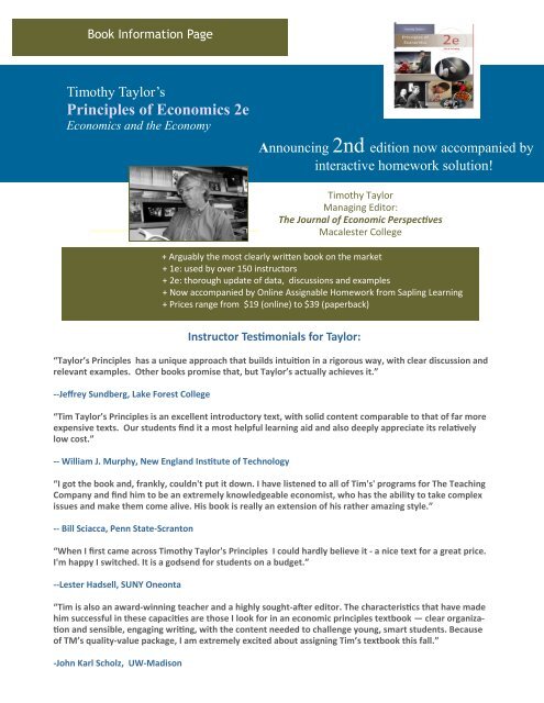
<strong>Book</strong> <strong>Information</strong> Page<br />
Timothy Taylor’s<br />
Principles of Economics 2e<br />
Economics and the Economy<br />
Announcing 2nd edition now accompanied by<br />
interactive homework solution!<br />
Timothy Taylor<br />
Managing Editor:<br />
The Journal of Economic Perspectives<br />
Macalester College<br />
+ Arguably the most clearly written book on the market<br />
+ 1e: used by over 150 instructors<br />
+ 2e: thorough update of data, discussions and examples<br />
+ Now accompanied by Online Assignable Homework from Sapling Learning<br />
+ Prices range from $19 (online) to $39 (paperback)<br />
Instructor Testimonials for Taylor:<br />
“Taylor’s Principles has a unique approach that builds intuition in a rigorous way, with clear discussion and<br />
relevant examples. Other books promise that, but Taylor’s actually achieves it.”<br />
--Jeffrey Sundberg, Lake Forest College<br />
“Tim Taylor’s Principles is an excellent introductory text, with solid content comparable to that of far more<br />
expensive texts. Our students find it a most helpful learning aid and also deeply appreciate its relatively<br />
low cost.”<br />
-- William J. Murphy, New England Institute of Technology<br />
“I got the book and, frankly, couldn't put it down. I have listened to all of Tim's' programs for The Teaching<br />
Company and find him to be an extremely knowledgeable economist, who has the ability to take complex<br />
issues and make them come alive. His book is really an extension of his rather amazing style.”<br />
-- Bill Sciacca, Penn State-Scranton<br />
“When I first came across Timothy Taylor's Principles I could hardly believe it - a nice text for a great price.<br />
I'm happy I switched. It is a godsend for students on a budget.”<br />
--Lester Hadsell, SUNY Oneonta<br />
“Tim is also an award-winning teacher and a highly sought-after editor. The characteristics that have made<br />
him successful in these capacities are those I look for in an economic principles textbook — clear organization<br />
and sensible, engaging writing, with the content needed to challenge young, smart students. Because<br />
of TM’s quality-value package, I am extremely excited about assigning Tim’s textbook this fall.”<br />
-John Karl Scholz, UW-Madison
Tim Taylor’s Principles of Economics 2e Page 2<br />
About the author/book:<br />
Tim Taylor’s career has been devoted to making complex economic ideas clear to students,<br />
policy makers and other professional economists. Taylor is the founding and only<br />
managing editor of the American Economic Association’s Journal of Economic Perspectives,<br />
which for more than 20 years has been an accessible source for state-of-the art<br />
economic thinking. Tim has won numerous teaching awards from his teaching stints at<br />
institutions like Stanford, the University of Minnesota and Macalester College.<br />
More about Tim Taylor’s Principles of Economics 2e (and Macro/Micro splits):<br />
<br />
<br />
<br />
<br />
<br />
<br />
<br />
<br />
<br />
<br />
Taylor 2e is a mainstream book; it covers all the main topics in a balanced way<br />
Taylor writes about the subject with no ideological axe to grind.<br />
<strong>Book</strong> is remarkably well written with clear examples; comprehensive, but no fluff.<br />
Focus on helping students solve problems – Taylor walks students through the problem-solving process.<br />
Coverage of international issues is integrated throughout, not tacked on as an afterthought.<br />
Treats the 2008 meltdown conceptually through the use of building blocks: bubbles, the housing market,<br />
the lender of last resort, banking, and what the Fed can do (quantitative easing).<br />
Careful attention to the budget deficit, the role that government spending can play in stimulating short-term<br />
growth, and how to think about the long-term implications.<br />
In micro section, "topics" chapters allow faculty to extend and apply analysis in the areas of their choice.<br />
Student Problems/Solutions manual is no-nonsense – lots of good problems that require drawing graphs<br />
and writing answers.<br />
Now accompanied by Sapling Learning’s interactive homework solution! www.saplinglearning.com<br />
<strong>Chapter</strong> 1: The Interconnected Economy<br />
<strong>Chapter</strong> 2: Choice in a World of Scarcity<br />
<strong>Chapter</strong> 3: International Trade<br />
<strong>Chapter</strong> 4: Demand and Supply<br />
<strong>Chapter</strong> 5: Labor and Financial Capital Markets<br />
<strong>Chapter</strong> 6: Globalization and Protectionism<br />
<strong>Chapter</strong> 7: Elasticity<br />
<strong>Chapter</strong> 8: Household Decision Making<br />
<strong>Chapter</strong> 9: Cost and Industry Structure<br />
<strong>Chapter</strong> 10: Perfect Competition<br />
<strong>Chapter</strong> 11: Monopoly<br />
<strong>Chapter</strong> 12: Monopolistic Competition and Oligopoly<br />
<strong>Chapter</strong> 13: Competition and Public Policy<br />
<strong>Chapter</strong> 14: Environmental Protection and Negative Externalities<br />
<strong>Chapter</strong> 15: Technology, Positive Externalities, and Public Goods<br />
<strong>Chapter</strong> 16: Poverty and Economic Inequality<br />
<strong>Chapter</strong> 17: Issues in Labor Markets: Unions, Discrimination,<br />
Immigration<br />
<strong>Chapter</strong> 18: <strong>Information</strong>, Risk and Insurance<br />
<strong>Chapter</strong> 19: Financial Markets<br />
<strong>Chapter</strong> 20: Public Choice<br />
For Instructors:<br />
Test Item File<br />
Computerized Test Bank<br />
Power Point Slides<br />
(Distributed on a Compact Disk)<br />
<strong>Chapter</strong> 21: The Macroeconomic Perspective<br />
<strong>Chapter</strong> 22: Economic Growth<br />
<strong>Chapter</strong> 23: Unemployment<br />
<strong>Chapter</strong> 24: Inflation<br />
<strong>Chapter</strong> 25: The Balance of Trade<br />
<strong>Chapter</strong> 26: The Aggregate Supply-Aggregate Demand<br />
<strong>Chapter</strong> 27: The Keynesian Perspective<br />
<strong>Chapter</strong> 28: The Neoclassical Perspective<br />
<strong>Chapter</strong> 29: Money and Banks<br />
<strong>Chapter</strong> 30: Monetary Policy and Bank Regulation<br />
<strong>Chapter</strong> 31: Exchange Rates and International Capital Flows<br />
<strong>Chapter</strong> 32: Government Budgets and Fiscal Policy<br />
<strong>Chapter</strong> 33: Government Borrowing and National<br />
<strong>Chapter</strong> 34: Macroeconomic Policy around the World<br />
Appendix to <strong>Chapter</strong> 1: Interpreting Graphics<br />
Appendix to <strong>Chapter</strong> 8: Indifference Curves<br />
Appendix to <strong>Chapter</strong> 19: Present Discounted Value<br />
Appendix to <strong>Chapter</strong> 27: An Algebraic Approach to the<br />
Expenditure-Output Model<br />
To Review Online <strong>Textbook</strong>:<br />
www.textbookmedia.com<br />
To Request Paperback:<br />
info@textbookmedia.com
Tim Taylor’s Principles of Economics 2e Page 3<br />
A sampling of the types of colleges/universities that are assigning Taylor:<br />
Columbia U, Eastern Michigan U; Lansing CC; U-Wisconsin, Madison; Grinnell College; Pima CC; Saint Olaf’s College;<br />
U of Arkansas; Duke U; NYU; DePaul U; U-Tennessee-Knoxville; Occidental College; U-Mass-Amherst; Georgia<br />
State U; Fitchburg State U; Carnegie Mellon U; Baruch College; Bellevue CC; Spelman College; Ashland U;<br />
Northwestern U; Normandale CC; Saddleback College; Cornell U; Johnson State U; Land of Lincoln CC; Beloit College;<br />
Pomona College; Augusta State U; Penn State-Scranton; Mesa CC; St. Paul College; U of Minnesota-Morris;<br />
U of California-Santa Barbara; Lake Forest College; Pitzer College; U of Montana; Penn; SUNY Oneonta; New<br />
Mexico Highlands CC; Bethel College; Temple U; U Nebraska-Omaha; Arizona State U; U of Rochester; UW-<br />
Milwaukee; Cal State-San Jose; St. Scholastica; U-Washington-Bothel; Pitt; UT-Dallas; U of Vermont; U of Alabama;<br />
Zane State U; U of Hawaii-Monoa; Colby College; Endicott College; Cal State LA; Georgia Southwestern;<br />
Claremont McKenna College; U of South Carolina; Lansing Community College; Indiana U of PA<br />
Affordable Student <strong>Textbook</strong> Options<br />
Online <strong>Book</strong>: $21.95<br />
Mobile Bundle: Online <strong>Book</strong>\iPhone: $23.95<br />
Digital Bundle (<strong>PDF</strong> + Online) $31.95<br />
Hybrid Bundle (Paperback +Online) $44.95<br />
Student Study Tools<br />
Online Problem Set: $6.95<br />
Printable Problem Set: $9.95<br />
<strong>PDF</strong> Flashcards: $8.95<br />
StudyUpGrade*: $9.95<br />
*Layers interactive quizzing, e-flash cards and<br />
key concept reviews into online textbook.
Demand and<br />
Supply<br />
When people talk about prices, the discussion often takes a judgmental<br />
tone. A bidder in an auction pays thousands of dollars for a dress once<br />
worn by Diana, Princess of Wales. A collector spends thousands of<br />
dollars for some drawings by John Lennon of the Beatles. Mouths gape. Surely<br />
such purchases are a waste of money? But when economists talk about prices, they<br />
are less interested in making judgments than in gaining a practical understanding<br />
of what determines prices and why prices change. In 1933, the great British<br />
economist Joan Robinson (1903–1983) explained how economists perceive price:<br />
The point may be put like this: You see two men, one of whom is giving a<br />
banana to the other, and is taking a penny from him. You ask, How is it that<br />
a banana costs a penny rather than any other sum? The most obvious line of<br />
attack on this question is to break it up into two fresh questions: How does<br />
it happen that the one man will take a penny for a banana? and: How does it<br />
happen that the other man will give a penny for a banana? In short, the natural<br />
thing is to divide up the problem under two heads: Supply and Demand.<br />
As a contemporary example, consider a price often listed on large signs beside<br />
well-traveled roads: the price of a gallon of gasoline. Why was the average price<br />
of gasoline in the United States $1.77 per gallon in January 2009? Why did the<br />
price for gasoline rise to $2.60 per gallon six months later by June 2009? To<br />
explain why prices are at a certain level and why that level changes over time,<br />
economic analysis focuses on the determinants of what gasoline buyers are willing<br />
to pay and what gasoline sellers are willing to accept. For example, the price of<br />
a gallon of gasoline in June of a given year is nearly always higher than the price<br />
in January of that year; over recent decades, gasoline prices in midsummer have<br />
averaged about 10 cents per gallon more than their midwinter low. The likely<br />
59
60 <strong>Chapter</strong> 4 Demand and Supply<br />
reason is that people want to drive more in the summer, and thus they are willing to pay<br />
more for gas at that time. However, in 2009, gasoline prices rose by much more than the<br />
average winter-to-summer rise, which suggests that other factors related to those who<br />
buy gasoline and firms that sell it changed during those six months, too.<br />
This chapter introduces the economic model of demand and supply. The discussion<br />
begins by examining how demand and supply determine the price and the quantity sold in<br />
markets for goods and services, and how changes in demand and supply lead to changes<br />
in prices and quantities. Then in <strong>Chapter</strong> 5, the very same demand and supply model<br />
is applied to markets for labor and financial capital. In <strong>Chapter</strong> 6, the same supply and<br />
demand model is applied to international trade. In situation after situation, in different<br />
places around the world, across different cultures, even reaching back into history, the<br />
demand and supply model offers a useful framework for thinking about what determines<br />
the prices and quantities of what is bought and sold.<br />
Demand, Supply, and Equilibrium in Markets<br />
for Goods and Services<br />
Markets for goods and services include everything from accounting services, air travel,<br />
and apples to zinc, zinfandel wine, and zucchini. Let’s first focus on what economists<br />
mean by demand, what they mean by supply, and then how demand and supply interact<br />
in an economic model of the market.<br />
Demand for Goods and Services<br />
Economists use the term demand to refer to a relationship between price and the<br />
quantity demanded. Price is what a buyer pays (or the seller receives) for a unit of the<br />
specific good or service. Quantity demanded refers to the total number of units that<br />
are purchased at that price. A rise in price of a good or service almost always decreases<br />
the quantity demanded of that good or service; conversely, a fall in price will increase<br />
the quantity demanded. When the price of a gallon of gasoline goes up, for example,<br />
people look for ways to reduce their purchases of gasoline by combining several errands,<br />
commuting by carpool or mass transit, or taking weekend or vacation trips by car close<br />
to home. Economists refer to the relationship that a higher price leads to a lower quantity<br />
demanded as the law of demand.<br />
Exhibit 4-1 gives an example in the market for gasoline. The table which shows<br />
the quantity demanded at each price is called a demand schedule. Price in this case<br />
is measured per gallon of gasoline. The quantity demanded is measured in millions<br />
of gallons over some time period (for example, per day or per year) and over some<br />
geographic area (like a state or a country). A demand curve shows the relationship<br />
between price and quantity demanded on a graph, with quantity on the horizontal axis<br />
and the price per gallon on the vertical axis. The demand schedule shown by the table and<br />
the demand curve shown on the graph are two ways of describing the same relationship<br />
between price and quantity demanded.<br />
Each individual good or service needs to be graphed on its own demand curve,<br />
because it wouldn’t make sense to graph the quantity of apples and the quantity of<br />
oranges on the same diagram. Demand curves will appear somewhat different for each<br />
product; for example, they may appear relatively steep or flat, or they may be straight<br />
or curved. But nearly all demand curves share the fundamental similarity that they<br />
demand: A relationship<br />
between price and the<br />
quantity demanded of a<br />
certain good or service.<br />
quantity demanded: The<br />
total number of units of a<br />
good or service purchased at<br />
a certain price.<br />
law of demand: The<br />
common relationship that a<br />
higher price leads to a lower<br />
quantity demanded of a<br />
certain good or service.<br />
demand schedule: A table<br />
that shows a range of prices<br />
for a certain good or service<br />
and the quantity demanded<br />
at each price.<br />
demand curve: A line<br />
that shows the relationship<br />
between price and quantity<br />
demanded of a certain good<br />
or service on a graph, with<br />
quantity on the horizontal<br />
axis and the price on the<br />
vertical axis.
<strong>Chapter</strong> 4 Demand and Supply<br />
61<br />
In economic terminology, demand is not the same as quantity demanded. When economists<br />
refer to demand, they mean the relationship between a range of prices and the quantities<br />
demanded at those prices, as illustrated by a demand curve or a demand schedule.<br />
When economists refer to quantity demanded, they often mean only a certain point on<br />
the demand curve, or perhaps the horizontal axis of the demand curve or one column of<br />
the demand schedule.<br />
Clearing It Up<br />
Demand Is Not Quantity<br />
Demanded<br />
Price ($ per gallon)<br />
$2.20<br />
$2.00<br />
$1.80<br />
$1.60<br />
$1.40<br />
$1.20<br />
$1.00<br />
D<br />
($2.20 per gallon, 420 million gallons)<br />
($2.00 per gallon, 460 million gallons)<br />
($1.80 per gallon, 500 million gallons)<br />
($1.60 per gallon, 550 million gallons)<br />
($1.40 per gallon, 600 million gallons)<br />
($1.20 per gallon, 700 million gallons)<br />
300 400 500 600 700 800 900<br />
Quantity of Gasoline (millions of gallons)<br />
($1.00 per gallon, 800 million gallons)<br />
Price (per gallon) Quantity demanded (in millions of gallons)<br />
$1.00 800<br />
$1.20 700<br />
$1.40 600<br />
$1.60 550<br />
$1.80 500<br />
$2.00 460<br />
$2.20 420<br />
Exhibit 4-1 A Demand<br />
Curve for Gasoline<br />
The table that shows quantity<br />
demanded of gasoline at<br />
each price is called a demand<br />
schedule. The demand<br />
schedule shows that as price<br />
rises, quantity demanded<br />
decreases. These points are<br />
then graphed on the figure,<br />
and the line connecting<br />
them is the demand curve<br />
D. The downward slope of<br />
the demand curve again<br />
illustrates the pattern that<br />
as price rises, quantity<br />
demanded decreases. This<br />
pattern is called the law of<br />
demand.<br />
slope down from left to right. In this way, demand curves embody the law of demand;<br />
as the price increases, the quantity demanded decreases, and conversely, as the price<br />
decreases, the quantity demanded increases.<br />
Supply of Goods and Services<br />
When economists talk about supply, they are referring to a relationship between price<br />
received for each unit sold and the quantity supplied, which is the total number of<br />
units sold in the market at a certain price. A rise in price of a good or service almost<br />
always leads to an increase in the quantity supplied of that good or service, while a<br />
fall in price will decrease the quantity supplied. When the price of gasoline rises, for<br />
example, profit-seeking firms are encouraged to expand exploration for oil reserves;<br />
to carry out additional drilling for oil; to make new investments in pipelines and oil<br />
tankers to bring the oil to plants where it can be refined into gasoline; to build new oil<br />
refineries; to purchase additional pipelines and trucks to ship the gasoline to gas stations;<br />
and to open more gas stations or to keep existing gas stations open longer hours. The<br />
supply: A relationship<br />
between price and the<br />
quantity supplied of a certain<br />
good or service.<br />
quantity supplied: The<br />
total number of units of a<br />
good or service sold at a<br />
certain price.
62 <strong>Chapter</strong> 4 Demand and Supply<br />
In economic terminology, supply is not the same as quantity supplied. When economists<br />
refer to supply, they mean the relationship between a range of prices and the quantities<br />
supplied at those prices, a relationship that can be illustrated with a supply curve or a<br />
supply schedule. When economists refer to quantity supplied, they often mean only a<br />
certain point on the supply curve, or sometimes, they are referring to the horizontal axis<br />
of the supply curve or one column of the supply schedule.<br />
Clearing It Up<br />
Supply Is Not the Same<br />
as Quantity Supplied<br />
Price ($ per gallon)<br />
$2.20<br />
$2.00<br />
$1.80<br />
$1.60<br />
$1.40<br />
$1.20<br />
$1.00<br />
300 400 500 600 700 800 900<br />
Quantity of Gasoline (millions of gallons)<br />
($2.20 per gallon, 720 million gallons)<br />
($2.00 per gallon, 700 million gallons)<br />
($1.80 per gallon, 680 million gallons)<br />
($1.60 per gallon, 640 million gallons)<br />
($1.40 per gallon, 600 million gallons)<br />
($1.20 per gallon, 550 million gallons)<br />
($1.00 per gallon, 500 million gallons)<br />
Price (per gallon)<br />
Quantity supplied (millions of gallons)<br />
$1.00 500<br />
$1.20 550<br />
$1.40 600<br />
$1.60 640<br />
$1.80 680<br />
$2.00 700<br />
$2.20 720<br />
Exhibit 4-2 A Supply<br />
Curve for Gasoline<br />
The supply schedule is the<br />
table that shows quantity<br />
supplied of gasoline at each<br />
price. As price rises, quantity<br />
supplied also increases. The<br />
supply curve S is created by<br />
graphing the points from the<br />
supply schedule and then<br />
connecting them. The upward<br />
slope of the supply curve<br />
illustrates the pattern that a<br />
higher price leads to a higher<br />
quantity supplied—a pattern<br />
that is common enough to be<br />
called the law of supply.<br />
pattern that a higher price is associated with a greater quantity supplied is so common<br />
that economists have named it the law of supply.<br />
Exhibit 4-2 illustrates the law of supply, again using the market for gasoline as an<br />
example. A supply schedule is a table that shows the quantity supplied at a range of<br />
different prices. Again, price is measured per gallon of gasoline and quantity demanded<br />
is measured in millions of gallons. A supply curve is a graphical illustration of the<br />
relationship between price, shown on the vertical axis, and quantity, shown on the<br />
horizontal axis. The supply schedule and the supply curve are just two different ways<br />
of showing the same information. Notice that the horizontal and vertical axes on the<br />
graph for the supply curve are the same as for the demand curve.<br />
Just as each product has its own demand curve, each product has its own supply<br />
curve. The shape of supply curves will vary somewhat according to the product: steeper,<br />
flatter, straighter, or curved. But nearly all supply curves share a basic similarity: they<br />
slope up from left to right. In that way, the supply curve illustrates the law of supply:<br />
as the price rises, the quantity supplied increases, and conversely, as the price falls, the<br />
quantity supplied decreases.<br />
law of supply: The common<br />
relationship that a higher<br />
price is associated with a<br />
greater quantity supplied.<br />
supply schedule: A table<br />
that shows a range of prices<br />
for a good or service and the<br />
quantity supplied at each<br />
price.<br />
supply curve: A line that<br />
shows the relationship<br />
between price and quantity<br />
supplied on a graph, with<br />
quantity supplied on the<br />
horizontal axis and price on<br />
the vertical axis.
<strong>Chapter</strong> 4 Demand and Supply<br />
63<br />
Equilibrium—Where Demand and Supply Cross<br />
Because the graphs for demand and supply curves both have price on the vertical axis<br />
and quantity on the horizontal axis, the demand curve and supply curve for a particular<br />
good or service can appear on the same graph. Together, demand and supply determine<br />
the price and the quantity that will be bought and sold in a market.<br />
Exhibit 4-3 illustrates the interaction of demand and supply in the market for<br />
gasoline. The demand curve D is identical to Exhibit 4-1. The supply curve S is identical<br />
to Exhibit 4-2. When one curve slopes down, like demand, and another curve slopes<br />
up, like supply, the curves intersect at some point.<br />
In every economics course you will ever take, when two lines on a diagram<br />
cross, this intersection means something! The point where the supply curve S and the<br />
demand curve D cross, designated by point E in Exhibit 4-3, is called the equilibrium.<br />
The equilibrium price is defined as the price where quantity demanded is equal to<br />
quantity supplied. The equilibrium quantity is the quantity where quantity demanded<br />
and quantity supplied are equal at a certain price. In Exhibit 4-3, the equilibrium price<br />
is $1.40 per gallon of gasoline and the equilibrium quantity is 600 million gallons. If<br />
you had only the demand and supply schedules, and not the graph, it would be easy<br />
to find the equilibrium by looking for the price level on the tables where the quantity<br />
demanded and the quantity supplied are equal.<br />
The word equilibrium means “balance.” If a market is balanced at its equilibrium<br />
price and quantity, then it has no reason to move away from that point. However, if a<br />
market is not balanced at equilibrium, then economic pressures arise to move toward<br />
the equilibrium price and the equilibrium quantity.<br />
equilibrium price:<br />
The price where quantity<br />
demanded is equal to quantity<br />
supplied.<br />
equilibrium quantity: The<br />
quantity at which quantity<br />
demanded and quantity<br />
supplied are equal at a<br />
certain price.<br />
equilibrium: The<br />
combination of price and<br />
quantity where there is no<br />
economic pressure from<br />
surpluses or shortages that<br />
would cause price or quantity<br />
to shift.<br />
P ($ per gallon)<br />
$2.20<br />
$1.80<br />
$1.40<br />
$1.20<br />
$1.00<br />
Excess supply<br />
or surplus<br />
$0.60<br />
300 400 500 600 700 800 900<br />
Quantity of Gasoline (millions of gallons)<br />
E<br />
Price (per gallon) Quantity demanded Quantity supplied<br />
$1.00 800 500<br />
$1.20 700 550<br />
$1.40 600 600<br />
$1.60 550 640<br />
$1.80 500 680<br />
$2.00 460 700<br />
$2.20 420 720<br />
S<br />
An above-equilibrium price<br />
Equilibrium price<br />
A below-equilibrium price<br />
Excess demand<br />
or shortage<br />
D<br />
Exhibit 4-3 Demand<br />
and Supply for Gasoline<br />
The demand curve D and<br />
the supply curve S intersect<br />
at the equilibrium point E,<br />
with a price of $1.40 and<br />
a quantity of 600. The<br />
equilibrium is the only price<br />
where quantity demanded is<br />
equal to quantity supplied.<br />
At a price above equilibrium<br />
like $1.80, quantity supplied<br />
of 680 exceeds the quantity<br />
demanded of 500, so there is<br />
excess supply or a surplus.<br />
At a price below equilibrium<br />
such as $1.20, quantity<br />
demanded of 700 exceeds<br />
quantity supplied of 550, so<br />
there is excess demand or a<br />
shortage.
64 <strong>Chapter</strong> 4 Demand and Supply<br />
Imagine, for example, that the price of a gallon of gasoline was above the<br />
equilibrium price; that is, instead of $1.40 per gallon, the price is $1.80 per gallon.<br />
This above-equilibrium price is illustrated by the dashed horizontal line at the price of<br />
$1.80 in Exhibit 4-3. At this higher price of $1.80, the quantity demanded drops from<br />
the equilibrium quantity of 600 to 500. This decline in quantity reflects how people<br />
and businesses react to the higher price by seeking out ways to use less gasoline, like<br />
sharing rides to work, taking mass transit, and avoiding faraway vacation destinations.<br />
Moreover, at this higher price of $1.80, the quantity supplied of gasoline rises from the<br />
600 to 680, as the higher price provides incentives for gasoline producers to expand<br />
their output. At this above-equilibrium price, there is excess supply, or a surplus;<br />
that is, the quantity supplied exceeds the quantity demanded at the given price. With a<br />
surplus, gasoline accumulates at gas stations, in tanker trucks, in pipelines, and at oil<br />
refineries. This accumulation puts pressure on gasoline sellers. If a surplus of gasoline<br />
remains unsold, those firms involved in making and selling gasoline are not receiving<br />
enough cash to pay their workers and to cover their expenses. In this situation, at least<br />
some gasoline producers and sellers will be tempted to cut prices, because it’s better<br />
to sell at a lower price than not to sell at all. Once some sellers start cutting gasoline<br />
prices, others will follow so that they won’t lose sales to the earlier price-cutters. These<br />
price reductions in turn will stimulate a higher quantity demanded. Thus, if the price is<br />
above the equilibrium level, incentives built into the structure of demand and supply<br />
will create pressures for the price to fall toward the equilibrium.<br />
Now suppose that the price is below its equilibrium level at $1.20 per gallon, as<br />
shown by the dashed horizontal line at this price in Exhibit 4-3. At this lower price, the<br />
quantity demanded increases from 600 to 700 as drivers take longer trips, spend more<br />
minutes warming up their car in the driveway in wintertime, stop sharing rides to work,<br />
and buy larger cars that get fewer miles to the gallon. However, the below-equilibrium<br />
price reduces gasoline producers’ incentives to produce and sell gasoline, and the quantity<br />
supplied of gasoline falls from 600 to 550. When the price is below equilibrium, there is<br />
excess demand, or a shortage; that is, at the given price the quantity demanded, which<br />
has been stimulated by the lower price, now exceeds the quantity supplied, which had<br />
been depressed by the lower price. In this situation, eager gasoline buyers mob the gas<br />
stations, only to find many stations running short of fuel. Oil companies and gas stations<br />
recognize that they have an opportunity to make higher profits by selling what gasoline<br />
they have at a higher price. As a result, the price increases toward the equilibrium level.<br />
excess supply: When at<br />
the existing price, quantity<br />
supplied exceeds the quantity<br />
demanded; also called a<br />
“surplus.”<br />
surplus: When at the<br />
existing price, quantity<br />
supplied exceeds the quantity<br />
demanded; also called<br />
“excess supply.”<br />
excess demand: At the<br />
existing price, the quantity<br />
demanded exceeds the<br />
quantity supplied, also called<br />
“shortage.”<br />
shortage: At the existing<br />
price, the quantity demanded<br />
exceeds the quantity<br />
supplied, also called “excess<br />
demand.”<br />
Shifts in Demand and Supply for Goods and<br />
Services<br />
A demand curve shows how quantity demanded changes as the price rises or falls.<br />
A supply curve shows how quantity supplied changes as the price rises or falls. But<br />
what happens when factors other than price influence quantity demanded and quantity<br />
supplied? For example, what if demand for, say, vegetarian food becomes popular<br />
with more consumers? Or what if the supply of, say, diamonds rises not because of<br />
any change in price, but because companies discover several new diamond mines? A<br />
change in price leads to a different point on a specific demand curve or a supply curve,<br />
but a shift in some economic factor other than price can cause the entire demand curve<br />
or supply curve to shift.
<strong>Chapter</strong> 4 Demand and Supply<br />
65<br />
The Ceteris Paribus Assumption<br />
A demand curve or a supply curve is a relationship between two and only two variables:<br />
quantity on the horizontal axis and price on the vertical axis. Thus, the implicit<br />
assumption behind a demand curve or a supply curve is that no other relevant economic<br />
factors are changing. Economists refer to this assumption as ceteris paribus, a Latin<br />
phrase meaning “other things being equal.” Any given demand or supply curve is based<br />
on the ceteris paribus assumption that all else is held equal. If all else is not held equal,<br />
then the demand or supply curve itself can shift.<br />
An Example of a Shifting Demand Curve<br />
The original demand curve D 0<br />
in Exhibit 4-4 shows at point Q that at a price of $20,000<br />
per car, the quantity of cars demanded would be 18 million. The original demand curve<br />
D 0<br />
also shows how the quantity of cars demanded would change as a result of a higher<br />
or lower price; for example, if the price of a car rose to $22,000, the quantity demanded<br />
would decrease to 17 million, as at point R.<br />
The original demand curve D 0<br />
, like every demand curve, is based on the ceteris<br />
paribus assumption that no other economically relevant factors change. But now imagine<br />
that the economy expands in a way that raises the incomes of many people. As a result<br />
of the higher income levels, a shift in demand occurs, which means that compared to<br />
the original demand curve D 0<br />
, a different quantity of cars will now be demanded at every<br />
ceteris paribus: Other<br />
things being equal.<br />
shift in demand: When a<br />
change in some economic<br />
factor related to demand<br />
causes a different quantity to<br />
be demanded at every price.<br />
$28,000<br />
Exhibit 4-4 Shifts in<br />
Demand: A Car Example<br />
Increased demand means<br />
that at every given price,<br />
the quantity demanded is<br />
higher, so that the demand<br />
curve shifts to the right from<br />
D 0<br />
to D 1<br />
. Decreased demand<br />
means that at every given<br />
price, the quantity demand<br />
is lower, so that the demand<br />
curve shifts to the left from D 0<br />
to D 2<br />
.<br />
Price<br />
$26,000<br />
$24,000<br />
$22,000<br />
$20,000<br />
$18,000<br />
$16,000<br />
$14,000<br />
p = 20,000<br />
q = 14.4 million<br />
T<br />
R<br />
p = 20,000<br />
q = 18 million<br />
Q<br />
p = 20,000<br />
q = 20 million<br />
S<br />
D 2<br />
D 0<br />
D 1<br />
$12,000<br />
$10,000<br />
8 13 14.4 17 18 20 23<br />
28<br />
Quantity<br />
Price<br />
Decrease<br />
to D 2<br />
Original Quantity<br />
Demanded D 0<br />
Increase<br />
to D 1<br />
$16,000 17.6 million 22.0 million 24.0 million<br />
$18,000 16.0 million 20.0 million 22.0 million<br />
$20,000 14.4 million 18.0 million 20.0 million<br />
$22,000 13.6 million 17.0 million 19.0 million<br />
$24,000 13.2 million 16.5 million 18.5 million<br />
$26,000 12.8 million 16.0 million 18.0 million
66 <strong>Chapter</strong> 4 Demand and Supply<br />
price. On the original demand curve, a price of $20,000 means a quantity demanded of<br />
18 million, but after higher incomes cause an increase in demand, a price of $20,000<br />
leads to a quantity demanded of 20 million, at point S. Exhibit 4-4 illustrates the shift in<br />
demand as a result of higher income levels with the shift of the original demand curve<br />
D 0<br />
to the right to the new demand curve D 1<br />
.<br />
This logic works in reverse, too. Imagine that the economy slows down so that many<br />
people lose their jobs or work fewer hours and thus suffer reductions in income. In this<br />
case, the shift in demand would lead to a lower quantity of cars demanded at every given<br />
price, and the original demand curve D 0<br />
would shift left to D 2<br />
. The shift from D 0<br />
to D 2<br />
represents a decrease in demand; that is, at any given price level, the quantity demanded<br />
is now lower. In this example, a price of $20,000 means 18 million cars sold along the<br />
original demand curve, but only 14.4 million cars sold after demand has decreased.<br />
When a demand curve shifts, it does not mean that the quantity demanded by every<br />
individual buyer changes by the same amount. In this example, not everyone would<br />
have higher or lower income and not everyone would buy or not buy an additional car.<br />
Instead, a shift in a demand captures an overall pattern for the market as a whole.<br />
Factors That Shift Demand Curves<br />
A change in any one of the underlying factors that determine what quantity people are<br />
willing to buy at a given price will cause a shift in demand. Graphically, the new demand<br />
curve lies either to the right or to the left of the original demand curve. Various factors<br />
may cause a demand curve to shift: changes in income, change in population, changes<br />
in taste, changes in expectations, and changes in the prices of closely related goods.<br />
Let’s consider these factors in turn.<br />
A change in income will often move demand curves. A household with a higher<br />
income level will tend to demand a greater quantity of goods at every price than a<br />
household with a lower income level. For some luxury goods and services, such as<br />
expensive cars, exotic spa vacations, and fine jewelry, the effect of a rise in income<br />
can be especially pronounced. However, a few exceptions to this pattern do exist. As<br />
incomes rise, many people will buy fewer popsicles and more ice cream, less chicken<br />
and more steak, they will be less likely to rent an apartment and more likely to own<br />
a home, and so on. Normal goods are defined as those where the quantity demanded<br />
rises as income rises, which is the most common case; inferior goods are defined as<br />
those where the quantity demanded falls as income rises.<br />
Changes in the composition of the population can also shift demand curves for<br />
certain goods and services. The proportion of elderly citizens in the U.S. population<br />
is rising from 9.8% in 1970, to 12.6% in 2000, and to a projected (by the U.S. Census<br />
Bureau) 20% of the population by 2030. A society with relatively more children, like<br />
the United States in the 1960s, will have greater demand for goods and services like<br />
tricycles and day care facilities. A society with relatively more elderly persons, as the<br />
United States is projected to have by 2030, has a higher demand for nursing homes<br />
and hearing aids.<br />
Changing tastes can also shift demand curves. In demand for music, for example,<br />
50% of sound recordings sold in 1990 were in the rock or pop music categories. By<br />
2007, rock and pop had fallen to 43% of the total, while sales of rap/ hip-hop, religious,<br />
and country categories had increased. Tastes in food and drink have changed, too. From<br />
1980 to 2007, the per person consumption of chicken by Americans rose from 33 pounds<br />
per year to 61 pounds per year, and consumption of cheese rose from 17 pounds per<br />
year to 32 pounds per year. Changes like these are largely due to movements in taste,<br />
normal goods: Goods<br />
where the quantity demanded<br />
rises as income rises.<br />
inferior goods: Goods<br />
where the quantity demanded<br />
falls as income rises.
<strong>Chapter</strong> 4 Demand and Supply<br />
67<br />
which change the quantity of a good demanded at every price: that is, they shift the<br />
demand curve for that good.<br />
Changes in expectations about future conditions and prices can also shift the demand<br />
curve for a good or service. For example, if people hear that a hurricane is coming,<br />
they may rush to the store to buy flashlight batteries and bottled water. If people learn<br />
that the price of a good like coffee is likely to rise in the future, they may head for the<br />
store to stock up on coffee now.<br />
The demand curve for one good or service can be affected by changes in the prices<br />
of related goods. Some goods and services are substitutes for others, which means that<br />
they can replace the other good to some extent. For example, if the price of cotton rises,<br />
driving up the price of clothing, sheets, and other items made from cotton, then some<br />
people will shift to comparable goods made from other fabrics like wool, silk, linen,<br />
and polyester. A higher price for a substitute good shifts the demand curve to the right;<br />
for example, a higher price for tea encourages buying more coffee. Conversely, a lower<br />
price for a substitute good has the reverse effect.<br />
Other goods are complements for each other, meaning that the goods are often<br />
used together, so that consumption of one good tends to increase consumption of the<br />
other. Examples include breakfast cereal and milk; golf balls and golf clubs; gasoline<br />
and sports utility vehicles; and the five-way combination of bacon, lettuce, tomato,<br />
mayonnaise, and bread. If the price of golf clubs rises, demand for a complement good<br />
like golf balls decreases. A higher price for skis would shift the demand curve for a<br />
complement good like ski resort trips to the left, while a lower price for a complement<br />
has the reverse effect.<br />
substitutes: Goods that<br />
can replace each other to<br />
some extent, so that greater<br />
consumption of one good can<br />
mean less of the other.<br />
complements: Goods that<br />
are often used together, so<br />
that consumption of one<br />
good tends to increase<br />
consumption of the other.<br />
Summing Up Factors That Change Demand<br />
Six factors that can shift demand curves are summarized in Exhibit 4-5. The direction of<br />
the arrows indicates whether the demand curve shifts represent an increase in demand or<br />
a decrease in demand based on the six factors we just considered. Notice that a change<br />
in the price of the good or service itself is not listed among the factors that can shift a<br />
demand curve. A change in the price of a good or service causes a movement along a<br />
specific demand curve, and it typically leads to some change in the quantity demanded,<br />
but it doesn’t shift the demand curve. Notice also that in these diagrams, the demand<br />
curves are drawn without numerical quantities and prices on the horizontal and vertical<br />
axes. The demand and supply model can often be a useful conceptual tool even without<br />
attaching specific numbers.<br />
When a demand curve shifts, it will then intersect with a given supply curve at a<br />
different equilibrium price and quantity. But we are getting ahead of our story. Before<br />
discussing how changes in demand can affect equilibrium price and quantity, we first<br />
need to discuss shifts in supply curves.<br />
An Example of a Shift in a Supply Curve<br />
A supply curve shows how quantity supplied will change as the price rises and falls,<br />
based on the ceteris paribus assumption that no other economically relevant factors are<br />
changing. But if other factors relevant to supply do change, then the entire supply curve<br />
can shift. Just as a shift in demand is represented by a change in the quantity demanded<br />
at every price, a shift in supply means a change in the quantity supplied at every price.<br />
In thinking about the factors that affect supply, remember the basic motivation of firms:<br />
to earn profits. If a firm faces lower costs of production, while the prices for the output<br />
the firm produces remain unchanged, a firm’s profits will increase. Thus, when costs of<br />
shift in supply: When a<br />
change in some economic<br />
factor related to supply<br />
causes a quantity to be<br />
supplied at every price.
68 <strong>Chapter</strong> 4 Demand and Supply<br />
Exhibit 4-5 Some Factors That Shift Demand Curves<br />
The left-hand panel (a) offers a list of factors that can cause an increase in demand from D 0<br />
to D 1<br />
. The right-hand panel (b)<br />
shows how the same factors, if their direction is reversed, can cause a decrease in demand from D 0<br />
to D 1<br />
. For example,<br />
greater popularity of a good or service increases demand, causing a shift in the demand curve to the right, while lesser<br />
popularity of a good or service reduces demand, causing a shift of the demand curve to the left.<br />
Taste shift to greater popularity<br />
Population likely to buy rises<br />
Income rises (for a normal good)<br />
Price of substitutes rises<br />
Price of complements falls<br />
Future expectations<br />
D 1<br />
encourage buying<br />
D 0<br />
Taste shift to lesser popularity<br />
Population likely to buy drops<br />
Income drops (for a normal good)<br />
Price of substitutes falls<br />
Price of complements rises<br />
Future expectations<br />
D 0<br />
discourage buying<br />
D 1<br />
Price<br />
Price<br />
Quantity<br />
(a) Factors that increase demand<br />
Quantity<br />
(b) Factors that decrease demand<br />
production fall, a firm will supply a higher quantity at any given price for its output, and<br />
the supply curve will shift to the right. Conversely, if a firm faces an increased cost of<br />
production, then it will earn lower profits at any given selling price for its products. As<br />
a result, a higher cost of production typically causes a firm to supply a smaller quantity<br />
at any given price. In this case, the supply curve shifts to the left.<br />
As an example, imagine that supply in the market for cars is represented by S 0<br />
in<br />
Exhibit 4-6. The original supply curve, S 0<br />
, includes a point with a price of $20,000 and<br />
a quantity supplied of 18 million cars, labeled as point J, which represents the current<br />
market equilibrium price and quantity. If the price rises to $22,000 per car, ceteris<br />
paribus, the quantity supplied will rise to 20 million cars, as shown by point K on the<br />
S 0<br />
curve.<br />
Now imagine that the price of steel, an important ingredient in manufacturing cars,<br />
rises, so that producing a car has now become more expensive. At any given price for<br />
selling cars, car manufacturers will react by supplying a lower quantity. The shift of<br />
supply from S 0<br />
to S 1<br />
shows that at any given price, the quantity supplied decreases. In<br />
this example, at a price of $20,000, the quantity supplied decreases from 18 million<br />
on the original supply curve S 0<br />
to 16.5 million on the supply curve S 1<br />
, which is labeled<br />
as point L.<br />
Conversely, imagine that the price of steel decreases, so that producing a car becomes<br />
less expensive. At any given price for selling cars, car manufacturers can now expect<br />
to earn higher profits and so will supply a higher quantity. The shift of supply to the<br />
right from S 0<br />
to S 2<br />
means that at all prices, the quantity supplied has increased. In this<br />
example, at a price of $20,000, the quantity supplied increases from 18 million on the<br />
original supply curve S 0<br />
to 19.8 million on the supply curve S 2<br />
, which is labeled M.<br />
Factors That Shift Supply Curves<br />
A change in any factor that determines what quantity firms are willing to sell at a<br />
given price will cause a change in supply. Some factors that can cause a supply curve<br />
to shift include: changes in natural conditions, altered prices for inputs to production,<br />
new technologies for production, and government policies that affect production costs.
<strong>Chapter</strong> 4 Demand and Supply<br />
69<br />
$28,000<br />
Exhibit 4-6 Shifts in<br />
Supply: A Car Example<br />
Increased supply means<br />
that at every given price, the<br />
quantity supplied is higher, so<br />
that the supply curve shifts<br />
to the right from S 0<br />
to S 2<br />
.<br />
Decreased supply means that<br />
at every given price, quantity<br />
supplied of cars is lower, so<br />
that the supply curve shifts to<br />
the left from S 0<br />
to S 1<br />
.<br />
Price<br />
$26,000<br />
$24,000<br />
$22,000<br />
$20,000<br />
$18,000<br />
$16,000<br />
p = 20,000<br />
q = 18 million<br />
p = 20,000<br />
q = 16.5 million<br />
p = 20,000<br />
q = 19.8 million<br />
K<br />
L J M<br />
S 1<br />
S 0<br />
S 2<br />
$14,000<br />
$12,000<br />
$10,000<br />
8 13 16.5 18 19.8 23<br />
Quantity<br />
Price<br />
Decrease<br />
to S 1<br />
Original Quantity<br />
Supplied S 0<br />
Increase<br />
to S 2<br />
$16,000 10.5 million 12.0 million 13.2 million<br />
$18,000 13.5 million 15.0 million 16.5 million<br />
$20,000 16.5 million 18.0 million 19.8 million<br />
$22,000 18.5 million 20.0 million 22.0 million<br />
$24,000 19.5 million 21.0 million 23.1 million<br />
$26,000 20.5 million 22.0 million 24.2 million<br />
The cost of production for many agricultural products will be affected by changes in<br />
natural conditions. For example, the area of northern China which typically grows about<br />
60% of the country’s wheat output experienced its worst drought in at least 50 years in<br />
the second half of 2009. A drought decreases the supply of agricultural products, which<br />
means that at any given price a lower quantity will be supplied; conversely, especially<br />
good weather would shift the supply curve to the right.<br />
Goods and services are produced using combinations of labor, materials, and<br />
machinery. When the price of a key input to production changes, the supply curve is<br />
affected. For example, a messenger company that delivers packages around a city may<br />
find that buying gasoline is one of its main costs. If the price of gasoline falls, then in the<br />
market for messenger services, a higher quantity will be supplied at any given price per<br />
delivery. Conversely, a higher price for key inputs will cause supply to shift to the left.<br />
When a firm discovers a new technology, so that it can produce at a lower cost,<br />
the supply curve will shift as well. For example, in the 1960s a major scientific effort<br />
nicknamed the Green Revolution focused on breeding improved seeds for basic crops<br />
like wheat and rice. By the early 1990s, more than two-thirds of the wheat and rice<br />
in low income countries around the world was grown with these Green Revolution<br />
seeds—and the harvest was twice as high per acre. A technological improvement that<br />
reduces costs of production will shift supply to the right, so that a greater quantity will<br />
be produced at any given price.
70 <strong>Chapter</strong> 4 Demand and Supply<br />
Government policies can affect the cost of production and the supply curve through<br />
taxes, regulations, and subsidies. For example, the U.S. government imposes a tax on<br />
alcoholic beverages that collects about $8 billion per year from producers. There is a<br />
wide array of government regulations that require firms to spend money to provide a<br />
cleaner environment or a safer workplace. A government subsidy, on the other hand,<br />
occurs when the government sends money to a firm directly or when the government<br />
reduces the firm’s taxes if the firm carries out certain actions. For example, the U.S.<br />
government pays more than $20 billion per year directly to firms to support research and<br />
development. From the perspective of a firm, taxes or regulations are an additional cost<br />
of production that shifts supply to the left, leading the firm to produce a lower quantity<br />
at every given price. However, government subsidies reduce the cost of production and<br />
increase supply.<br />
Summing Up Factors That Change Supply<br />
Natural disasters, changes in the cost of inputs, new technologies, and the impact of<br />
government decisions all affect the cost of production for firms. In turn, these factors<br />
affect firms’ willingness to supply at a given price. Exhibit 4-7 summarizes factors that<br />
change the supply of goods and services. Notice that a change in the price of the product<br />
itself is not among the factors that shift the supply curve. Although a change in price<br />
of a good or service typically causes a change in quantity supplied along the supply<br />
curve for that specific good or service, it does not cause the supply curve itself to shift.<br />
Because demand and supply curves appear on a two-dimensional diagram with only<br />
price and quantity on the axes, an unwary visitor to the land of economics might be<br />
fooled into believing that economics is only about four topics: demand, supply, price,<br />
and quantity. However, demand and supply are really “umbrella” concepts: demand<br />
covers all of the factors that affect demand, and supply covers all of the factors that<br />
affect supply. The factors other than price that affect demand and supply are included<br />
by using shifts in the demand or the supply curve. In this way, the two-dimensional<br />
demand and supply model becomes a powerful tool for analyzing a wide range of<br />
economic circumstances.<br />
Exhibit 4-7 Some Factors That Shift Supply Curves<br />
The right-hand panel (a) offers list of factors that can cause an increase in supply from S 0<br />
to S 1<br />
. The left-hand panel (b)<br />
shows that the same factors, if their direction is reversed, can cause a decrease in supply from S 0<br />
to S 1<br />
.<br />
Price<br />
Favorable natural conditions for<br />
production<br />
A fall in input prices<br />
Improved technology<br />
Lower product<br />
taxes/ less costly<br />
regulations<br />
S 0<br />
S 1<br />
Price<br />
Poor natural conditions for<br />
production<br />
A rise in input prices<br />
A decline in technology<br />
(not common)<br />
Higher product taxes/<br />
more costly<br />
regulations<br />
S 1<br />
S 0<br />
Quantity<br />
(a) Factors that increase supply<br />
Quantity<br />
(b) Factors that decrease supply
<strong>Chapter</strong> 4 Demand and Supply<br />
71<br />
Shifts in Equilibrium Price and Quantity:<br />
The Four-Step Process<br />
Let’s begin with a single economic event. It might be an event that affects demand,<br />
like a change in income, population, tastes, prices of substitutes or complements, or<br />
expectations about future prices. It might be an event that affects supply, like a change<br />
in natural conditions, input prices, or technology, or government policies that affect<br />
production. How does this economic event affect equilibrium price and quantity? We<br />
can analyze this question using a four-step process.<br />
Step 1: Think about what the demand and supply curves in this market looked like<br />
before the economic change occurred. Sketch the curves.<br />
Step 2: Decide whether the economic change being analyzed affects demand or supply.<br />
Step 3: Decide whether the effect on demand or supply causes the curve to shift to the<br />
right or to the left, and sketch the new demand or supply curve on the diagram.<br />
Step 4: Compare the original equilibrium price and quantity to the new equilibrium<br />
price and quantity.<br />
To make this process concrete, let’s consider one example that involves a shift in supply<br />
and one that involves a shift in demand.<br />
Good Weather for Salmon Fishing<br />
In summer 2000, weather conditions were excellent for commercial salmon fishing<br />
off the California coast. Heavy rains meant higher than normal levels of water in the<br />
rivers, which helps the salmon to breed. Slightly cooler ocean temperatures stimulated<br />
growth of plankton, the microscopic organisms at the bottom of the ocean food chain,<br />
thus providing everything in the ocean with a hearty food supply. The ocean stayed<br />
calm during fishing season, so commercial fishing operations didn’t lose many days to<br />
bad weather. How did these weather conditions affect the quantity and price of salmon?<br />
Exhibit 4-8 uses the four-step approach to work through this problem.<br />
1. Draw a demand and supply diagram to show what the market for salmon looked<br />
like before the good weather arrived. The original equilibrium E 0<br />
was $3.25 per<br />
pound and the original equilibrium quantity was 250,000 fish. (This price per pound<br />
is what commercial buyers pay at the fishing docks; what consumers pay at the<br />
grocery is higher.)<br />
2. Did the economic event affect supply or demand? Good weather is a natural condition<br />
that affects supply.<br />
3. Was the effect on supply an increase or a decrease? Good weather increases the<br />
quantity that will be supplied at any given price. The supply curve shifts to the right<br />
from the S 0<br />
to S 1<br />
.<br />
4. Compare the new equilibrium price and quantity to the original equilibrium. At the<br />
new equilibrium, E 1<br />
, the equilibrium price fell from $3.25 to $2.50, but the equilibrium<br />
quantity increased from 250,000 salmon to 550,000 fish. Notice that the equilibrium<br />
quantity demanded increased, even though the demand curve did not move.
72 <strong>Chapter</strong> 4 Demand and Supply<br />
Price ($ per pound)<br />
Price<br />
per Pound<br />
$4.00<br />
$3.50<br />
$3.00<br />
$2.50<br />
$2.00<br />
$1.50<br />
$1.00<br />
$0.50<br />
S 0<br />
$0.00<br />
0 200 400 600 800 1,000<br />
Quantity (thousands of fish)<br />
Quantity Supplied<br />
in 1999<br />
E 0<br />
(p = 3.25, q = 250)<br />
Quantity Supplied<br />
in 2000<br />
Quantity<br />
Demanded<br />
$2.00 80 400 840<br />
$2.25 120 480 680<br />
$2.50 160 550 550<br />
$2.75 200 600 450<br />
$3.00 230 640 350<br />
$3.25 250 670 250<br />
$3.50 270 700 200<br />
In short, good weather conditions increased supply for the California commercial<br />
salmon fishing industry. The result was a higher equilibrium quantity of salmon bought<br />
and sold in the market at a lower price.<br />
Seal Hunting and New Drugs<br />
As the catch of whales dwindled, Canada’s seal industry had become the only remaining<br />
large-scale hunt for marine mammals. In the late 1990s, about 280,000 Canadian seals<br />
were killed each year. In 2000, the number dropped to 90,000 seals. What happened?<br />
One major use of seals was that some of their body parts were used as ingredients in<br />
traditional medications in China and other Asian nations that promised to treat male<br />
impotence. However, pharmaceutical companies—led by Pfizer Inc., which invented<br />
the drug Viagra—developed some alternative and medically proven treatments for male<br />
impotence. How would the invention of Viagra, and other drugs to treat mail impotence,<br />
affect the harvest of seals? Exhibit 4-9 illustrates the four-step analysis.<br />
S 1<br />
E 1<br />
(p = 2.50, q = 550)<br />
D 0<br />
Exhibit 4-8 Good<br />
Weather for Salmon<br />
Fishing: The Four-Step<br />
Process<br />
Step 1: Draw a demand and<br />
supply diagram to illustrate<br />
what the market for salmon<br />
looked like in the year before<br />
the good weather arrived.<br />
The demand curve D 0<br />
and<br />
the supply curve S 0<br />
show that<br />
the original equilibrium price<br />
is $3.25 per pound and the<br />
original equilibrium quantity is<br />
250,000 fish.<br />
Step 2: Will the change<br />
described affect supply or<br />
demand? Good weather is an<br />
example of a natural condition<br />
that affects supply.<br />
Step 3: Will the effect on<br />
supply be an increase or<br />
decrease? Good weather is a<br />
change in natural conditions<br />
that increases the quantity<br />
supplied at any given price.<br />
The supply curve shifts to<br />
the right, moving from the<br />
original supply curve S 0<br />
to the<br />
new supply curve S 1<br />
, which is<br />
shown in both the schedule<br />
and the figure.<br />
Step 4: Compare the new<br />
equilibrium price and quantity<br />
to the original equilibrium.<br />
At the new equilibrium E 1<br />
,<br />
the equilibrium price falls<br />
from $3.25 to $2.50, but the<br />
equilibrium quantity increases<br />
from 250,000 to 550,000<br />
salmon.<br />
1. Draw a demand and supply diagram to illustrate what the market for seals looked like<br />
in the year before the invention of Viagra. In Exhibit 4-9, the demand curve D 0<br />
and the<br />
supply curve S 0<br />
show the original relationships. In this case, the analysis is performed<br />
without specific numbers on the price and quantity axes. (Not surprisingly, detailed<br />
annual data on quantities and prices of seals body parts are not readily available.)
<strong>Chapter</strong> 4 Demand and Supply<br />
73<br />
Price<br />
S 0<br />
E 0<br />
p 0<br />
E 1<br />
p 1<br />
D 0<br />
Exhibit 4-9 The Seal<br />
Market: A Four-Step Analysis<br />
Step 1: Draw a demand and<br />
supply diagram to illustrate what<br />
the market for seals looked like<br />
in the year before the invention<br />
of Viagra. The demand curve D 0<br />
and the supply curve S 0<br />
show the<br />
original relationships.<br />
Step 2: Will the change<br />
described affect supply or<br />
demand? A newly available<br />
substitute good, like Viagra, will<br />
affect demand for the original<br />
product, seals.<br />
q 1<br />
q 0<br />
Quantity<br />
2. Did the change described affect supply or demand? A newly available substitute<br />
good, like Viagra, will affect demand for the original product, seal body parts.<br />
3. Was the effect on demand an increase or a decrease? An effective substitute product<br />
for male impotence, means a lower quantity demanded of the original product at<br />
every given price, causing the demand curve for seals to shift left to the new demand<br />
curve D 1<br />
.<br />
4. Compare the new equilibrium price and quantity at E 1<br />
to the original equilibrium<br />
price and quantity at E 0<br />
. The new equilibrium E 1<br />
occurs at a lower quantity and a<br />
lower price than the original equilibrium E 0<br />
.<br />
D 1<br />
Step 3: Will the effect on<br />
demand be positive or negative?<br />
A less expensive substitute<br />
product will tend to mean a<br />
lower quantity demanded of the<br />
original product, seal, at every<br />
given price, causing the demand<br />
curve for seal to shift to the left<br />
from D 0<br />
to D 1<br />
.<br />
Step 4: Compare the new<br />
equilibrium price and quantity to<br />
the original equilibrium price. The<br />
new equilibrium E 1<br />
occurs at a<br />
lower quantity and a lower price<br />
than the original equilibrium E 0<br />
.<br />
The extremely sharp decline in the number of Canadian seals killed in the late 1990s,<br />
together with anecdotal evidence that the price of seal body parts dropped sharply at<br />
this time, suggests that the invention of drugs to treat male impotence helped reduce the<br />
number of seals killed. In fact, some environmentalists are hoping that such drugs may<br />
reduce demand for other common ingredients for traditional male potency medicines,<br />
including tiger bones and monkey heads.<br />
The Interconnections and Speed of Adjustment in Real Markets<br />
In the real world, many factors that affect demand and supply can change all at once. For<br />
example, the demand for cars might increase because of rising incomes and population,<br />
and it might decrease because of rising gasoline prices (a complementary good).<br />
Likewise, the supply of cars might increase because of innovative new technologies that<br />
reduce the cost of car production, and it might decrease as a result of new government<br />
regulations requiring the installation of costly pollution-control technology. Moreover,<br />
rising incomes and population or changes in gasoline prices will affect many markets,<br />
not just cars. How can an economist sort out all of these interconnected events? The<br />
answer lies in the ceteris paribus assumption. Look at how each economic event affects<br />
each market, one event at a time, holding all else constant.
74 <strong>Chapter</strong> 4 Demand and Supply<br />
One common mistake in applying the demand and supply framework is to confuse the<br />
shift of a demand or a supply curve with the movement along a demand or supply curve.<br />
As an example, consider a problem that asks whether a drought will increase or decrease<br />
the equilibrium quantity and equilibrium price of wheat. Lee, a student in an introductory<br />
economics class, might reason:<br />
“Well, it’s clear that a drought reduces supply, so I’ll shift back the supply curve, as in<br />
the shift from the original supply curve S 0<br />
to S 1<br />
shown on the diagram (call this Shift 1). So<br />
the equilibrium moves from E 0<br />
to E 1<br />
, the equilibrium quantity is lower and the equilibrium<br />
price is higher. Then, a higher price makes farmers more likely to supply the good, so the<br />
supply curve shifts right, as shown by the shift from S 1<br />
to S 2<br />
on the diagram (shown as<br />
Shift 2), so that the equilibrium now moves from E 1<br />
to E 2<br />
. But the higher price also reduces<br />
demand and so causes demand to shift back, like the shift from the original demand curve<br />
D 0<br />
to D 1<br />
on the diagram (labeled Shift 3), and the equilibrium moves<br />
from E 2<br />
to E 3<br />
.”<br />
At about this point, Lee suspects that this answer is headed<br />
down the wrong path. Think about what might be wrong with Lee’s<br />
logic, and then read the answer that follows.<br />
Answer: Lee’s first step is correct: that is, a drought shifts<br />
back the supply curve of wheat and leads to a prediction of a lower<br />
equilibrium quantity and a higher equilibrium price. The rest of<br />
Lee’s argument is wrong, because it mixes up shifts in supply with<br />
quantity supplied, and shifts in demand with quantity demanded. A<br />
higher or lower price never shifts the supply curve, as suggested by<br />
the shift in supply from S 1<br />
to S 2<br />
. Instead, a price change leads to a<br />
movement along a given supply curve. Similarly, a higher or lower<br />
price never shifts a demand curve, as suggested in the shift from D 0<br />
to D 1<br />
. Instead, a price change leads to a movement along a given<br />
demand curve. Remember, a change in the price of a good never<br />
causes the demand or supply curve for that good to shift.<br />
Price<br />
Clearing It Up<br />
Shifts of Demand<br />
or Supply versus<br />
Movements along a<br />
Demand or Supply<br />
Curve<br />
S 2<br />
S 0<br />
E 1<br />
Shift 1<br />
E 2<br />
Shift 2<br />
E 0<br />
Shift 3<br />
S 1<br />
D 0<br />
Quantity<br />
D 1<br />
In the four-step analysis of how economic events affect equilibrium price and<br />
quantity, the movement from the old to the new equilibrium seems immediate. But<br />
as a practical matter, prices and quantities often do not zoom straight to equilibrium.<br />
More realistically, when an economic event causes demand or supply to shift, prices<br />
and quantities set off in the general direction of equilibrium. Indeed, even as they are<br />
moving toward one new equilibrium, prices are often then pushed by another change<br />
in demand or supply toward another equilibrium.<br />
Price Ceilings and Price Floors in Markets for<br />
Goods and Services<br />
Controversy often surrounds the prices and quantities that are established by demand<br />
and supply. After all, every time you buy a gallon of gasoline, pay the rent for your<br />
apartment, or pay the interest charges on your credit card, it’s natural to wish that the<br />
price had been at least a little lower. Every time a restaurant sells a meal, a department<br />
store sells a sweater, or a farmer sells a bushel of wheat, it’s natural for the profit-seeking<br />
seller to wish that the price had been higher. In some cases, discontent over prices turns<br />
into public pressure on politicians, who may then pass legislation to prevent a certain<br />
price from climbing “too high” or falling “too low.” The demand and supply model
<strong>Chapter</strong> 4 Demand and Supply<br />
75<br />
What’s a Price Bubble? A Story of Housing Prices<br />
According to data from the Federal Housing Finance<br />
Agency, the average price of a U.S. single-family home<br />
rose about 1–3% per year in the first half of the 1990s;<br />
3–5% per year in the second half of the 1990s; 7–8% per<br />
year in the early 2000s; and more than 10% per year from<br />
late 2004 to early 2006.<br />
Although no one seriously expected price increases<br />
of 10% per year to continue for long, what happened next<br />
was still a shock. Although certain metropolitan areas or<br />
states had seen declines in housing prices from time to<br />
time, there had not been a nationwide decline in housing<br />
prices since the Great Depression of the 1930s. But housing<br />
prices started falling in 2006, and through much of 2008<br />
and 2009, housing prices were falling at a rate of 4–5%<br />
per year. Of course, these national averages understate<br />
the experience of certain parts of the country where both<br />
the boom and the bust were much larger.<br />
Economists refer to this chain of events as a price<br />
“bubble.” Remember that one possible reason for demand<br />
to shift is expectations about the future. If many people<br />
expect that housing prices are going to rise in the future,<br />
demand for housing will shift to the right—thus helping<br />
the prediction of higher prices come true. For a time, a<br />
cycle of expecting higher prices, increases in demand,<br />
and resulting higher prices can be self-reinforcing. But this<br />
process cannot last forever. At some unpredictable time,<br />
many people recognize that the expectations of ever-higher<br />
future prices are unrealistic, at which point demand shifts<br />
back in the other direction and the price bubble deflates.<br />
Price bubbles are not just observed in housing: they are<br />
also seen from time in markets for collectible items, and<br />
in stock markets.<br />
The bursting of the price bubble in housing—which<br />
happened in many countries around the world, not just<br />
the United States—has caused great economic difficulties.<br />
Those who owned homes watched the value of this asset<br />
decline. Some of those who borrowed money to buy a<br />
house near the peak of the bubble found a few years later,<br />
after the bubble had burst, that what they owed to the bank<br />
was much more than the house was worth. When many<br />
people began to default on their mortgage loans, banks<br />
and other financial institutions then faced huge losses. The<br />
bursting of the price bubble in housing helped to trigger the<br />
global economic slowdown that started in 2008.<br />
shows how people and firms will react to the incentives provided by these laws to control<br />
prices, in ways that will often lead to undesirable costs and consequences. Alternative<br />
policy tools can often achieve the desired goals of price control laws, while avoiding<br />
at least some of the costs and trade-offs of such laws.<br />
Price Ceilings<br />
Price controls are laws that the government enacts to regulate prices. Price controls<br />
come in two flavors. A price ceiling keeps a price from rising above a certain level,<br />
while a price floor keeps a price from falling below a certain level. This section uses<br />
the demand and supply framework to analyze price ceilings; the next section turns to<br />
price floors.<br />
In many markets for goods and services, demanders outnumber suppliers. There<br />
are more people who buy bread than companies that make bread; more people who rent<br />
apartments than landlords; more people who purchase prescription drugs than companies<br />
that manufacture such drugs; more people who buy gasoline than companies that refine<br />
and sell gasoline. Consumers, who are also potential voters, sometimes unite behind a<br />
political proposal to hold down a certain price. In some cities, for example, renters have<br />
pressed political leaders to pass rent control laws, a form of price ceiling that usually<br />
works by stating that rents can only be raised by a certain maximum percentage each year.<br />
Rent control can become a politically hot topic when rents begin to rise rapidly.<br />
Rents might rise for many reasons. Perhaps a change in tastes makes a certain suburb<br />
or town a more popular place to live. Perhaps locally based businesses expand, bringing<br />
higher incomes and more people into the area. Changes of this sort can cause a change<br />
in the demand for rental housing, as illustrated in Exhibit 4-10. The original equilibrium<br />
E 0<br />
lies at the intersection of supply curve S 0<br />
and demand curve D 0<br />
, corresponding to an<br />
price controls: Government<br />
laws to regulate prices.<br />
price ceiling: A law that<br />
prevents a price from rising<br />
above a certain level.<br />
price floor: A law that<br />
prevents a price from falling<br />
below a certain level.
76 <strong>Chapter</strong> 4 Demand and Supply<br />
Price<br />
Price (dollars in monthly rent)<br />
$900<br />
$800<br />
$700<br />
$600<br />
$500<br />
$400<br />
$300<br />
$200<br />
$100<br />
0<br />
Original Quantity<br />
Supplied<br />
D 0<br />
D 1<br />
E 0<br />
E 1<br />
Excess demand<br />
or shortage<br />
from price ceiling<br />
10 11 12 13 14 15 16 17 18 19 20 21 22 23 24<br />
Quantity (thousands of rental units)<br />
Original Quantity<br />
Demanded<br />
New Quantity<br />
Demanded<br />
$400 12,000 18,000 23,000<br />
$500 15,000 15,000 19,000<br />
$600 17,000 13,000 17,000<br />
$700 19,000 11,000 15,000<br />
$800 20,000 10,000 14,000<br />
S 0<br />
Price ceiling<br />
set here<br />
Exhibit 4-10 A Price<br />
Ceiling Example—Rent<br />
Control<br />
The original intersection of<br />
demand and supply occurs<br />
at E 0<br />
. Demand shifts from D 0<br />
to D 1<br />
. The new equilibrium<br />
would be at E 1<br />
—except that<br />
a price ceiling prevents the<br />
price from rising. Because<br />
the price doesn’t change, the<br />
quantity supplied remains<br />
at 15,000. However, after<br />
the change in demand, the<br />
quantity demanded rises<br />
to 19,000. There is excess<br />
demand, also called a<br />
shortage.<br />
equilibrium price of $500 and an equilibrium quantity of 15,000 units of rental housing.<br />
The effect of greater income or a change in tastes is to shift the demand curve for rental<br />
housing to the right, as shown by the data in the table and the shift from D 0<br />
to D 1<br />
on the<br />
graph. In this market, at the new equilibrium E 1<br />
, the price of a rental unit would rise to<br />
$600 and the equilibrium quantity would increase to 17,000 units.<br />
Long-time apartment dwellers will dislike these price increases. They may argue,<br />
“Why should our rents rise because a lot of newcomers want to move in?” The current<br />
apartment-dwellers are also voters, and they may elect local politicians who pass a price<br />
ceiling law that limits how much rents can rise.<br />
For simplicity, let’s assume that a rent control law is passed to keep the price at the<br />
original equilibrium of $500 for a typical apartment. In Exhibit 4-10, the horizontal<br />
line at the price of $500 shows the legally fixed maximum price set by the rent control<br />
law. However, the underlying forces that shifted the demand curve to the right have not<br />
vanished. At that price ceiling, the quantity demanded exceeds the quantity supplied:<br />
that is, at a price of $500 the quantity supplied remains at the same 15,000 rental units,<br />
but the quantity demanded is 19,000 rental units. Thus, people who would like to rent<br />
in this area are knocking on the doors of landlords, searching for apartments. A situation<br />
of excess demand, also called a shortage, results when people are willing to pay the<br />
market price but cannot purchase (or in this case rent) what they desire.<br />
Rent control has been especially popular in wartime and during times of high<br />
inflation. New York City, the most prominent U.S. city that has imposed rent control<br />
laws for a long period, put rent control in place as a “temporary” measure during World<br />
War II. Rent control was also especially popular during the 1970s, when all prices in<br />
the U.S. economy were rising rapidly as part of an overall process of inflation. By the<br />
mid-1980s, more than 200 American cities, with about 20% of the nation’s population,<br />
had rent control laws. But in the last two decades, the political pendulum began swinging
<strong>Chapter</strong> 4 Demand and Supply<br />
77<br />
against rent control. Thirty-one states adopted laws or constitutional amendments<br />
banning rent control outright. In many cities that kept some form of rent control, the<br />
focus of the law shifted from trying to hold rents below the equilibrium price to offering<br />
ways for resolving disputes between tenants and landlords, like disagreements about<br />
maintenance, pets, and noise. But in New York City, relatively strict rent controls have<br />
persisted into the 2000s.<br />
Although the effect of rent control laws in the United States has faded in recent years,<br />
price ceilings are often proposed for other products. For example, price ceilings to limit<br />
what producers can charge have been proposed in recent years for prescription drugs, on<br />
doctor and hospital fees, the charges made by some automatic teller bank machines, and<br />
auto insurance rates. Many low-income countries around the world, including nations in<br />
Africa and Asia, have also imposed price ceilings on basic items like bread. In the early<br />
2000s, the government of the African country of Zimbabwe tried to help its ordinary<br />
citizens by placing ceilings on the prices of ordinary household items like bread, wheat,<br />
and cooking oil. But many producers of these items, faced with the low prices, went<br />
out of business. The goal of the price ceiling had been to keep necessities affordable to<br />
all, but the result was that the quantity of the products declined and shortages occurred.<br />
Price ceilings are enacted in an attempt to keep prices low for those who demand<br />
the product. But when the market price is not allowed to rise to the equilibrium level,<br />
quantity demanded exceeds quantity supplied, and thus a shortage occurs. Those who<br />
manage to purchase the product at the lower price given by the price ceiling will benefit,<br />
but sellers of the product will suffer, along with those who are not able to purchase the<br />
product at all.<br />
Price Floors<br />
Price floors are enacted when discontented sellers, feeling that prices are too low, appeal<br />
to legislators to keep prices from falling. A price floor is the lowest legal price that can<br />
be paid in markets for goods and services, labor, and financial capital. Price floors are<br />
sometimes called “price supports,” because they support a price by preventing it from<br />
falling below a certain level.<br />
Around the world, many countries have passed laws to keep farm prices higher than<br />
they otherwise would be. In the annual budget of the European Union, roughly half of<br />
all spending late in the first decade of the 2000s—about $65 billion per year—is used<br />
to keep prices high for Europe’s farmers. Thanks to this policy, the prices received by<br />
European farmers for such agricultural staples as wheat, barley, rice, milk, and beef have<br />
held substantially above the price prevailing in the world market for several decades.<br />
Exhibit 4-11 illustrates the effects of a government program that assures a price<br />
above the equilibrium by focusing on the market for wheat in Europe. In the absence<br />
of government intervention, the price would adjust so that the quantity supplied would<br />
equal the quantity demanded at the equilibrium point E 0<br />
, with price p 0<br />
and quantity Q 0<br />
.<br />
However, policies to keep prices high for farmers keeps the price above what would<br />
have been the market equilibrium level—the price p f<br />
shown by the dashed horizontal<br />
line in the diagram. The result is a quantity supplied of Q S<br />
in excess of the quantity<br />
demanded Q d<br />
. When quantity supply exceeds quantity demanded, then a situation of<br />
excess supply exists, also called a surplus. The high-income countries of the world,<br />
including the United States, Europe and Japan, spend a total of about $1 billion per day<br />
in supporting their farmers. If the government is willing to purchase the excess supply<br />
(or to provide payments for others to purchase it), then farmers will benefit from the<br />
price floor but taxpayers and consumers of food will pay the costs. Numerous proposals<br />
have been offered for reducing farm subsidies. But in many countries, political support
78 <strong>Chapter</strong> 4 Demand and Supply<br />
Neither price ceilings nor price floors cause demand or supply to change. Remember,<br />
changes in price don’t cause demand or supply to change. Price ceilings and price floors<br />
can cause a different choice of quantity demanded along a demand curve, but they don’t<br />
move the demand curve. Price controls can cause a different choice of quantity supplied<br />
along a supply curve, but they don’t shift the supply curve.<br />
Clearing It Up<br />
Price Ceilings and<br />
Floors Do Not Change<br />
Demand or Supply<br />
In economics, (price) ceilings are graphically lower than (price) floors. The reason<br />
is that binding price ceilings are below the equilibrium level, stopping the price from<br />
rising, and binding price floors are above the equilibrium level, stopping the price<br />
from falling. So above-equilibrium price floors are higher than below-equilibrium<br />
price ceilings.<br />
Clearing It Up<br />
When Floors Are Higher<br />
Than Ceilings<br />
D<br />
S<br />
Exhibit 4-11 The<br />
European Wheat Prices:<br />
A Price Floor Example<br />
The intersection of demand D<br />
and supply S would be at the<br />
equilibrium point E 0<br />
. However,<br />
a price floor set at p f<br />
holds the<br />
price above E 0<br />
and prevents it<br />
from falling. The result of the<br />
price floor is that the quantity<br />
supplied Q s<br />
exceeds the<br />
quantity demanded Q d<br />
. There<br />
is excess supply, also called<br />
a surplus.<br />
Price<br />
p f<br />
Excess supply<br />
or surplus<br />
p 0<br />
E 0<br />
Price floor set here<br />
Q d<br />
Q 0<br />
Q S<br />
Quantity<br />
for subsidies for farmers—and indirectly, for what is viewed as the traditional rural way<br />
of life—remains strong.<br />
Responses to Price Controls: Many Margins for Action<br />
Although a government can set price floors or price ceilings, it cannot control how<br />
households and firms react to these price controls. Attempts to control prices often<br />
have unintended consequences. The focus of the discussion so far has been on reactions<br />
that take the form of changes in quantity demanded or quantity supplied, and thus on<br />
understanding why price ceilings commonly lead to shortages and price floors lead to<br />
surpluses. However, buyers and sellers in real-world markets have many other ways in<br />
which they can react to price controls. The ability of households and firms to react in a<br />
variety of ways to government rules is called the problem of “many margins for action.”<br />
One alternative reaction occurs when buyers and seller decide to break the government<br />
rules on prices or sales, which is referred to as black market. Consider a landlord who<br />
black market: An<br />
illegal market that breaks<br />
government rules on prices<br />
or sales.
<strong>Chapter</strong> 4 Demand and Supply<br />
79<br />
Price Controls of 1776<br />
During the American Revolution, a number of states<br />
imposed price ceilings on many goods. After Rhode Island<br />
passed price control laws in 1776, the city of Providence<br />
reported on the effects to the state legislature in 1777:<br />
[The effect] is so intricate, variable, and complicated,<br />
that it cannot remain any time equitable . . . It was<br />
made to cheapen the articles of life, but it has It was<br />
made to cheapen the articles of life, but it has in fact<br />
raised their prices, by producing an artificial and in<br />
some respects a real scarcity. It was made to unite<br />
us in good agreement respecting prices; but hath<br />
produced animosity, and ill will between town and<br />
country, and between buyers and sellers in general.<br />
It was made to bring us up to some equitable<br />
standard of honesty . . . but hath produced a<br />
sharping set of mushroom peddlars, who adulterate<br />
their commodities, and take every advantage to<br />
evade the . . . act, by quibbles and lies.<br />
Price control laws are often popular in the short run,<br />
because they look like an easy fix, but they become less<br />
popular over time as shortages occur, social tensions arise,<br />
and efforts to evade the laws gain force. The problems<br />
noted by the citizens of Providence, Rhode Island, in 1775<br />
apply today as they did more than 200 years ago.<br />
owns rent-controlled property. Suppose that although the law dictates the cap on the rent<br />
that the landlord can charge, a potential tenant is willing to pay more than the rent control<br />
law allows to live in the apartment. If this “extra rent” is paid in cash, then who will know?<br />
A second margin for action is “side payments,” which are additional payments that<br />
are made along with the actual price paid. In New York City, with its long history of<br />
rent control, landlords have devised innovative charges like a “nonrefundable cleaning<br />
deposit” and a “nonrefundable key deposit,” or they may require several months’ rent<br />
in advance. These charges can have the effect of making the tenant pay more than the<br />
actual rent.<br />
A third margin for action involves quality adjustment. In the case of rent control,<br />
a landlord may keep the rent low but put off needed maintenance or installing new<br />
appliances. The result is a lower-priced apartment—but also a lower-quality apartment.<br />
A fourth margin for action involves shifting who is involved in the transaction. In<br />
cities with rent control, it isn’t unusual for a tenant living in a rent-controlled apartment<br />
not to move out officially; instead, the tenant sublets the apartment to someone else. In<br />
this case, the original tenant pays the rent-controlled rate but charges the market rate to<br />
the new renter and pockets the difference.<br />
Those who favor price floors and price ceilings are often quite aware of the actions<br />
that can circumvent the underlying purpose of price controls. Thus, supporters of<br />
price controls also favor rules that will include penalties for black markets, make side<br />
payments illegal, require certain quality levels, and prohibit shifts in who is involved in<br />
the transaction. However, establishing rules or laws that will limit all of the alternative<br />
margins for action is like trying to block a flowing stream with your fingers. Shutting<br />
down the many margins for action by which citizens and firms respond to price controls<br />
is much easier said than done.<br />
Policy Alternatives to Price Ceilings and Price Floors<br />
The economic analysis of how price ceilings can create shortages and price floors<br />
create surpluses can be disheartening. If you want to pursue a policy goal of assuring<br />
that people have a sufficient quantity of affordable housing, but rent controls are just<br />
price ceilings that cause housing shortages, what alternative policy can you advocate? If<br />
you want to pursue a policy goal of supporting farmers, but farm price supports lead to<br />
storehouses of surplus grain rotting at high cost to taxpayers and consumers, then what<br />
alternative policy can you advocate? The same demand and supply model that shows
80 <strong>Chapter</strong> 4 Demand and Supply<br />
Price (dollars per housing unit)<br />
p 2<br />
p 3<br />
p 0<br />
p 1<br />
E 0<br />
E 3<br />
E 1<br />
D 1<br />
q 0<br />
q 1<br />
q 2<br />
q 3<br />
Quantity (housing units)<br />
that price ceilings and price floors often have unintended, undesirable consequences of<br />
creating surpluses and shortages, can also suggest alternate public policies that do not<br />
have these same trade-offs.<br />
Let’s return to the issue of rent control. If the goal is to have an expanded supply<br />
of affordable housing, then a rightward shift in a demand curve, a supply curve, or both<br />
as shown in Exhibit 4-12, can accomplish this goal. A shift to the right in the supply<br />
of affordable housing from S 0<br />
to S 1<br />
, for example, might be achieved if a government<br />
grants subsidies to builders who construct apartment buildings that include have<br />
relatively smaller rental units, which will have a more affordable price in the market.<br />
This step taken alone would cause a shift to the right from the original equilibrium,<br />
E 0,<br />
to the new equilibrium, E 1<br />
, and would increase the quantity of housing from q 0<br />
to<br />
q 1<br />
. A shift to the right in the demand curve from D 0<br />
to D 1<br />
might be achieved by giving<br />
a subsidy to low-income renters, perhaps in the form of cash or of a voucher that the<br />
renters could use to pay some of the rent, so that low-income renters could then have<br />
more to spend on housing. This step taken alone would cause a shift to the right from<br />
the original equilibrium, E 0<br />
, to the new equilibrium, E 2<br />
, and would increase the quantity<br />
of affordable housing from q 0<br />
to q 2<br />
. Instituting both sets of policies would shift supply<br />
from S 0<br />
to S 1<br />
, demand from D 0<br />
to D 1<br />
, the equilibrium from the original E 0<br />
to E 3<br />
, and the<br />
quantity of affordable housing from q 0<br />
to q 3<br />
.<br />
Any combination of these policies is likely to be more useful in expanding affordable<br />
housing than rent control, because these policies tend to increase the quantity of<br />
affordable housing, whereas rent control tends to decrease it. Moreover, these alternative<br />
policies sidestep many of the problems that arise when suppliers and demanders react<br />
to price controls.<br />
Similarly, there are a number of alternative policies to support farmers or rural<br />
areas that do not involve setting price floors for crops. For example, the government<br />
could provide income directly to farmers, especially to those with lower incomes.<br />
The government might also assist rural economies in many other ways: establishing<br />
new branches of state colleges and universities in agricultural areas, creating parks or<br />
D 0<br />
Exhibit 4-12 Policies<br />
for Affordable Housing:<br />
Alternatives to Rent<br />
Control<br />
The original equilibrium is the<br />
intersection of demand D 0<br />
and<br />
supply S 0<br />
at the equilibrium<br />
E 0<br />
. Providing subsidies to lowincome<br />
buyers of housing will<br />
shift the demand curve from<br />
D 0<br />
to D 1<br />
, leading to a new<br />
equilibrium at E 2<br />
. Alternatively,<br />
a policy of providing subsidies<br />
to builders of affordable<br />
housing would shift the<br />
supply curve from S 0<br />
to S 1<br />
,<br />
leading to a new equilibrium<br />
at E 1<br />
. Undertaking both<br />
demand-side and supplyside<br />
policies would move<br />
the market to equilibrium<br />
E 3<br />
, at the intersection of<br />
the new demand curve D 1<br />
and the new supply curve<br />
S 1<br />
. As drawn here, both of<br />
these policies will increase<br />
the equilibrium quantity<br />
of affordable housing. An<br />
increase in demand will also<br />
raise the price of affordable<br />
housing, but as long as the<br />
subsidy received by buyers is<br />
larger than the higher price,<br />
buyers will not be adversely<br />
affected by the higher price<br />
that occurs from an increase<br />
in demand.
<strong>Chapter</strong> 4 Demand and Supply<br />
81<br />
nature preserves that might attract tourists, supporting research into new methods of<br />
producing and using local crops to help the local farmers stay ahead, helping to build<br />
transportation links to rural areas, and subsidizing high-speed Internet cable connections<br />
across rural areas or wireless phone service. All of these alternative policies would help<br />
rural communities while avoiding the problem of price floors, because these alternative<br />
policies don’t encourage farmers to produce an excess supply of surplus food.<br />
With alternative policies like these readily available, why do governments enact<br />
price floors and price ceilings? One reason is that in public policy debates over<br />
price controls, people often don’t take into account the unintended but predictable<br />
tradeoffs. Another reason is that government sometimes views laws about price floors<br />
and ceilings as having zero cost, while giving subsidies to demanders or suppliers<br />
requires a government to collect taxes and spend money. The point here is not to<br />
endorse every proposal for using targeted subsidies or tax breaks to change demand<br />
and supply. Each policy proposal must be evaluated according to its own costs and<br />
benefits. But before reaching for the seemingly easy policy tool of price controls,<br />
with all of their undesired if predictable consequences and trade-offs, it is wise to<br />
consider alternative policies to shift demand and supply so as to achieve the desired<br />
new market equilibrium.<br />
Supply, Demand, and Efficiency<br />
In the market equilibrium, where the quantity demanded equals quantity supplied,<br />
nothing is wasted. No excess supply sits unsold, gathering dust in warehouses. No<br />
shortages exist that cause people to stand in long lines or rely on political connections<br />
to acquire goods—alternatives that involve wastes of time and energy. All those who<br />
wish to purchase or sell goods at the equilibrium market price are able to purchase or<br />
sell the quantity that they desire, as movements of the equilibrium price bring quantity<br />
demanded and supplied into balance.<br />
The familiar demand and supply diagram holds within it the concept of economic<br />
efficiency, which was introduced in <strong>Chapter</strong> 2. To economists, an efficient outcome is<br />
one where it is impossible to improve the situation of one party without imposing a cost<br />
on someone else. Conversely, if a situation is inefficient, it becomes possible to benefit<br />
at least one party without imposing costs on others. Thus, the definition of productive<br />
efficiency in <strong>Chapter</strong> 2 was that economy was producing without waste, and getting all<br />
it could out of its scarce resources, in the sense that it was impossible to get more of<br />
good A without a reduction in good B. Efficiency in the demand and supply model has<br />
the same basic meaning: the economy is getting as much benefit as possible from its<br />
scarce resources and all the possible gains from trade have been achieved.<br />
Consumer Surplus, Producer Surplus, Social Surplus<br />
Consider the example of a market for portable devices that can store and play digital<br />
music and other audio files shown in Exhibit 4-13. The equilibrium price is $80 and the<br />
equilibrium quantity is 28 million. To see the benefits received by consumers, look at the<br />
segment of the demand curve above the equilibrium point and to the left. This portion<br />
of the demand curve shows that at least some demanders would have been willing to<br />
pay more than $80 for a portable music player. For example, point J shows that if the<br />
price was $90, the quantity demanded of the portable music player would have been 20<br />
million. Those consumers who would have been willing to pay $100 for a portable music
82 <strong>Chapter</strong> 4 Demand and Supply<br />
Price<br />
$120<br />
$100<br />
$90<br />
$80<br />
$60<br />
$40<br />
$20<br />
F<br />
J<br />
Consumer surplus<br />
Producer surplus<br />
G<br />
10 14<br />
K<br />
20 28 30<br />
Quantity<br />
player based on the utility they expect to receive from it, but who were able to pay the<br />
equilibrium price of $80, clearly received a benefit. Remember, the demand curve traces<br />
out the willingness to pay for different quantities. The amount that individuals would<br />
have been willing to pay minus the amount that they actually paid is called consumer<br />
surplus. Consumer surplus is the area labeled F—that is, the area between the market<br />
price and the segment of the demand curve above equilibrium.<br />
The equilibrium price also benefits producers. The supply curve shows the quantity<br />
that firms are willing to supply at each price. For example, point K on Exhibit 4-13<br />
illustrates that at a price of $40, firms would still have been willing to supply a quantity<br />
of 14 million. Those producers who would have been willing to supply the portable<br />
music players at a price of $40, but who were instead able to charge the equilibrium<br />
price of $80, clearly received a benefit. Producer surplus is the amount that a seller<br />
is paid for a good minus the seller’s actual cost. In Exhibit 4-13, producer surplus is<br />
the area labeled G—that is, the area between the market price and the segment of the<br />
supply curve below the equilibrium.<br />
Social surplus is the sum of consumer surplus and producer surplus. In Exhibit 4-13,<br />
social surplus would thus be shown as the area F + G. Social surplus is larger at<br />
equilibrium quantity and price than it would be at any other quantity. At the efficient<br />
level of output, it is impossible to produce greater consumer surplus without reducing<br />
producer surplus, and it is impossible to produce greater producer surplus without<br />
reducing consumer surplus.<br />
Inefficiency of Price Floors and Price Ceilings<br />
The imposition of a price floor or a price ceiling will prevent a market from adjusting to<br />
its equilibrium price and quantity, and thus will create an inefficient outcome. But there<br />
is an additional twist here. Along with creating inefficiency, price floors and ceilings<br />
will also transfer some consumer surplus to producers, or some producer surplus to<br />
consumers. Let’s consider a price ceiling and a price floor in turn.<br />
E<br />
D<br />
S<br />
Figure 4-13 Consumer<br />
and Producer Surplus<br />
The triangular area labeled by<br />
F shows the area of consumer<br />
surplus, which shows that the<br />
equilibrium price in the market<br />
was less than what many of<br />
the consumers were willing<br />
to pay. For example, point J<br />
on the demand curve shows<br />
that even at the price of $90,<br />
consumers would have been<br />
willing to purchase a quantity<br />
of 20. But those consumers<br />
only needed to pay the<br />
equilibrium price of $80. The<br />
triangular area labeled by G<br />
shows the area of producer<br />
surplus, which shows that the<br />
equilibrium price received in<br />
the market was more than<br />
what many of the producers<br />
were willing to accept for<br />
their products. For example,<br />
point K on the supply curve<br />
shows that at a price of $40,<br />
firms would have been willing<br />
to supply a quantity of 14.<br />
However, in this market those<br />
firms could receive a price of<br />
$80 for their production. The<br />
sum of consumer surplus and<br />
producer surplus—that is, F +<br />
G—is called social surplus.<br />
consumer surplus: The<br />
benefit consumers receive<br />
from buying a good or<br />
service, measured by what<br />
the individuals would have<br />
been willing to pay minus<br />
the amount that they actually<br />
paid.<br />
producer surplus: The<br />
benefit producers receive<br />
from selling a good or service,<br />
measured by the price the<br />
producer actually received<br />
minus the price the producer<br />
would have been willing to<br />
accept.<br />
social surplus: The sum<br />
of consumer surplus and<br />
producer surplus.
<strong>Chapter</strong> 4 Demand and Supply<br />
83<br />
P<br />
$600<br />
$400<br />
X<br />
T<br />
V<br />
U<br />
W<br />
15,000 20,000<br />
Q<br />
(a) Reduced social surplus from a price ceiling<br />
S<br />
Price<br />
ceiling<br />
D<br />
P<br />
$12<br />
$8<br />
G<br />
H<br />
I<br />
J<br />
K<br />
Price<br />
floor<br />
1,400 1,800<br />
Q<br />
(b) Reduced social surplus from a price floor<br />
D<br />
S<br />
Figure 4-14 Efficiency<br />
and Price Floors and<br />
Ceilings<br />
(a) The original equilibrium<br />
price is $600 with a quantity<br />
of 20,000. Consumer surplus<br />
is T + U, and producer surplus<br />
is V + W + X. A price ceiling<br />
is imposed at $400, so firms<br />
in the market now produce<br />
only a quantity of 15,000. As<br />
a result, the new consumer<br />
surplus is T + V, while the<br />
new producer surplus is X.<br />
In effect, the price ceiling<br />
transfers the surplus V from<br />
producers to consumers, but<br />
also causes deadweight loss<br />
in social surplus of U + W.<br />
Imagine that several firms develop a promising but expensive new drug for treating<br />
back pain. If this therapy is left to the market, the equilibrium price will be $600 per<br />
month and 200,000 people will use the drug, as shown in Exhibit 4-14a. The original<br />
level of consumer surplus is the T + U and producer surplus is V + W + X. However, the<br />
government decides to impose a price ceiling of $400 to make the drug more affordable.<br />
At this price ceiling, firms in the market now produce only a quantity of 150,000. As a<br />
result, two changes occur. First, an inefficient outcome occurs and the total surplus of<br />
society is reduced. Deadweight loss is the name for the loss in social surplus that occurs<br />
when the economy produces at an inefficient quantity. In Exhibit 4-14a, the deadweight<br />
loss is the area U + W. When deadweight loss exists, it is possible for both consumer<br />
and producer surplus to increase, in this case because the price control is blocking some<br />
suppliers and demanders from transactions that they would both be willing to make. A<br />
second change from the price ceiling is that some of the producer surplus is transferred<br />
to consumers. After the price ceiling is imposed, the new consumer surplus is T + V,<br />
while the new producer surplus is X. In other words, the price ceiling transfers the area<br />
of surplus V from producers to consumers.<br />
For the case of a price floor shown in Exhibit 4-14b, envision a situation where a city<br />
with several movie theaters that are all losing money. The current equilibrium is a price<br />
of $8 per movie, with 1,800 people attending movies. The original consumer surplus<br />
is G + H + J, and producer surplus is I + K. The city government is worried that movie<br />
theaters will go out of business, thus reducing the entertainment options available to<br />
citizens, so it decides to impose a price floor of $12 per ticket. As a result, the quantity<br />
demanded of movie tickets falls to 1,400. The new consumer surplus is G, and the new<br />
producer surplus is H + I. In effect, the price floor causes the area H to be transferred<br />
from consumer to producer surplus, but also causes a deadweight loss of J + K.<br />
This analysis shows that a price ceiling, like a law establishing rent controls, will<br />
transfer some producer surplus to consumers—which helps to explain why consumers<br />
often favor them. Conversely, a price floor like a guarantee that farmers will receive a<br />
certain price for their crops will transfer some consumer surplus to producers, which<br />
explains why producers often favor them. However, both price floors and price ceilings<br />
block some transactions that buyers and sellers would have been willing to make, and<br />
(b) The original equilibrium<br />
is $8 at a quantity of 1,800.<br />
Consumer surplus is G + H<br />
+ J, and producer surplus is I<br />
+ K. A price floor is imposed<br />
at $12, which means that<br />
quantity demanded falls to<br />
1,400. As a result, the new<br />
consumer surplus is G, and<br />
the new producer surplus<br />
is H + I. In effect, the price<br />
floor causes the area H to be<br />
transferred from consumer<br />
to producer surplus, but also<br />
causes a deadweight loss in<br />
social surplus of J + K.<br />
deadweight loss: The loss<br />
in social surplus that occurs<br />
when a market produces an<br />
inefficient quantity.
84 <strong>Chapter</strong> 4 Demand and Supply<br />
create deadweight loss. Removing such barriers so that prices and quantities can adjust<br />
to their equilibrium level will increase the economy’s social surplus.<br />
Demand and Supply as a Social Adjustment<br />
Mechanism<br />
The demand and supply model emphasizes that prices are not set only by demand or<br />
only by supply, but by the interaction between the two. In 1890, the famous economist<br />
Alfred Marshall wrote that asking whether supply or demand determined a price was<br />
like arguing “whether it is the upper or the under blade of a pair of scissors that cuts a<br />
piece of paper.” The answer is that both blades of the demand and supply scissors are<br />
always involved.<br />
The adjustments of equilibrium price and quantity in a market-oriented economy<br />
often occur without much government direction or oversight. If the coffee crop in Brazil<br />
suffers a terrible frost, then the supply curve of coffee shifts to the left and the price of<br />
coffee rises. Some people—call them the coffee addicts—continue to drink coffee and<br />
pay the higher price. Others switch to tea or soft drinks. No government commission is<br />
needed to figure out how to adjust coffee prices; or which companies will be allowed<br />
to process the remaining supply; or which supermarkets in which cities will get how<br />
much coffee to sell; or which consumers will ultimately be allowed to drink the brew.<br />
Such adjustments in response to price changes happen all the time in a market economy,<br />
often so smoothly and rapidly that we barely notice them. Think for a moment of all<br />
the seasonal foods that are available and inexpensive at certain times of the year, like<br />
fresh corn in midsummer, but more expensive at other times of the year. People alter<br />
their diets and restaurants alter their menus in response to these fluctuations in prices<br />
without fuss or fanfare. For both the U.S. economy and the world economy as a whole,<br />
demand and supply is the primary social mechanism for answering the basic questions<br />
about what is produced, how it is produced, and for whom it is produced.<br />
Key Concepts and Summary<br />
1. A demand schedule is a table that shows the quantity demanded at different<br />
prices in the market. A demand curve shows the relationship between quantity<br />
demanded and price in a given market on a graph. The law of demand points out<br />
that a higher price typically leads to a lower quantity demanded.<br />
2. A supply schedule is a table that shows the quantity supplied at different prices<br />
in the market. A supply curve shows the relationship between quantity supplied<br />
and price on a graph. The law of supply points out that a higher price typically<br />
leads to a higher quantity supplied.<br />
3. The equilibrium price and equilibrium quantity occur where the supply and<br />
demand curves cross. The equilibrium occurs where the quantity demanded is<br />
equal to the quantity supplied.<br />
4. If the price is below the equilibrium level, then the quantity demanded will<br />
exceed the quantity supplied. Excess demand or a shortage will exist. If the
<strong>Chapter</strong> 4 Demand and Supply<br />
85<br />
price is above the equilibrium level, then the quantity supplied will exceed<br />
the quantity demanded. Excess supply or a surplus will exist. In either case,<br />
economic pressures will push the price toward the equilibrium level.<br />
5. Economists often use the ceteris paribus or “other things equal” assumption,<br />
that while examining the economic impact of one event, all other factors remain<br />
unchanged for the purpose of the analysis.<br />
6. Factors that can shift the demand curve for goods and services, causing a<br />
different quantity to be demanded at any given price, include changes in tastes,<br />
population, income, prices of substitute or complement goods, and expectations<br />
about future conditions and prices.<br />
7. Factors that can shift the supply curve for goods and services, causing a different<br />
quantity to be supplied at any given price, include natural conditions, input<br />
prices, changes in technology, and government taxes, regulations, or subsidies.<br />
8. When using the supply and demand framework to think about how an event will<br />
affect the equilibrium price and quantity, proceed through four steps: (a) Sketch<br />
a supply and demand diagram to think about what the market looked like before<br />
the event; (b) decide whether the event will affect supply or demand; (c) decide<br />
whether the effect on supply or demand is negative or positive, and draw the<br />
appropriate shifted supply or demand curve; (d) compare the new equilibrium<br />
price and quantity to the original ones.<br />
9. Price ceilings prevent a price from rising above a certain level. When a price<br />
ceiling is set below the equilibrium price, quantity demanded will exceed<br />
quantity supplied, and excess demand or shortages will result. Price floors<br />
prevent a price from falling below as certain level. When a price floor is set<br />
above the equilibrium price, quantity supplied will exceed quantity demanded,<br />
and excess supply or surpluses will result.<br />
10. Price floors and price ceilings often lead to unintended consequences, because<br />
buyers and sellers have many margins for action. These margins include black<br />
markets, side payments, quality adjustments, and shifts in who is involved in the<br />
transaction.<br />
11. Policies that shift supply and demand explicitly, through targeted subsidies or<br />
taxes, are often preferable to policies that attempt to set prices, because they<br />
avoid the shortages, surpluses, and other unintended consequences that price<br />
ceilings and floors typically produce.<br />
12. Consumer surplus is the gap between the price that consumers are willing to<br />
pay, based on their preferences, and the market equilibrium price. Producer<br />
surplus is the gap between the price for which producers are willing to sell a<br />
product, based on their costs, and the market equilibrium price. Social surplus<br />
is the sum of consumer surplus and producer surplus. Total surplus is larger at<br />
the equilibrium quantity and price than it will be at any other quantity and price.<br />
Deadweight loss is loss in total surplus that occurs when the economy produces<br />
at an inefficient quantity.
86 <strong>Chapter</strong> 4 Demand and Supply<br />
Review Questions<br />
1. In the economic view, what determines the level of<br />
prices?<br />
2. What does a downward-sloping demand curve<br />
mean about how buyers in a market will react to a<br />
higher price?<br />
3. Will demand curves have the same exact shape in<br />
all markets?<br />
4. What does an upward-sloping supply curve mean<br />
about how sellers in a market will react to a higher<br />
price?<br />
5. Will supply curves have the same shape in all<br />
markets?<br />
6. What is the relationship between quantity<br />
demanded and quantity supplied at equilibrium?<br />
7. How can you locate the equilibrium point on a<br />
demand and supply graph?<br />
8. When analyzing a market, how do economists deal<br />
with the problem that many factors that affect the<br />
market are changing at the same time?<br />
9. If the price is above the equilibrium level, would<br />
you predict excess supply or excess demand? If<br />
the price is below the equilibrium level, would you<br />
predict a shortage or a surplus?<br />
10. Explain why a price that is above the equilibrium<br />
level will tend to fall toward equilibrium. Explain<br />
why a price that is below the equilibrium level will<br />
tend to rise toward the equilibrium.<br />
11. Name some factors that can cause a shift in the<br />
demand curve in markets for goods and services.<br />
12. Does a price ceiling attempt to make a price higher<br />
or lower?<br />
13. How does a price ceiling set below the equilibrium<br />
level affect quantity demanded and quantity<br />
supplied?<br />
14. Does a price floor attempt to make a price higher or<br />
lower?<br />
15. How does a price floor set above the equilibrium<br />
level affect quantity demanded and quantity<br />
supplied?<br />
16. Make a list of ways that buyers and sellers may<br />
respond to price ceilings and price floors, other than<br />
changes in quantity.<br />
17. Why might economists commonly prefer public<br />
policies that shift demand and/or supply rather than<br />
imposing price ceilings or price floors?<br />
18. What’s the difference between demand and quantity<br />
demanded?<br />
19. Name some factors that can cause a shift in the<br />
supply curve in markets for goods and services.<br />
20. Is supply the same thing as quantity supplied?<br />
Explain.<br />
21. What is consumer surplus? How is it illustrated on<br />
a demand and supply diagram?<br />
22. What is producer surplus? How is it illustrated on a<br />
demand and supply diagram?<br />
23. What is total surplus? How is it illustrated on a<br />
demand and supply diagram?<br />
24. What is the relationship between total surplus and<br />
economic efficiency?<br />
25. What is deadweight loss?