Solved Problems Chapter 3: Mechanical Systems - KFUPM Open ...

ME 413: System Dynamics and Control
Dr. A. Aziz Bazoune
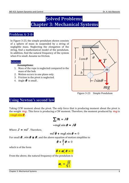
Problem A-3-8-
Solved Problems
Chapter 3: Mechanical Systems
In Figure 3-23, the simple pendulum shown consists
of a sphere of mass m suspended by a string of
negligible mass. Neglecting the elongation of the
string, find a mathematical model of the pendulum.
In addition, find the natural frequency of the system
when θ is small. Assume no friction.
Solution
Assumptions:
1. Mass of the rope is neglected compared to the
mass of the bob.
2. Motion occurs in one plane only.
3. Friction in the pivot is neglected.
4. Angle θ is small .
l
l cosθ
h
θ
T
l
m
lsinθ
mg
Figure 3-23
Simple Pendulum
Using Newton’s second law
Taking CCW moment about the pivot. The only force that is producing moment about the pivot is
the weight mg . This force is producing a CW moment. Therefore, the moment produced by mg is
− mgl sin θ .
M = J && θ
2
= ml . Therefore,
∑
− mgl sin
θ
=
J &&
θ
Where J
2
ml &&
θ
+ mgl sin
θ
=
0
For small θ , sin θ
≅
θ
, and the above equation of motion simplifies to
&& g
θ
+ θ
=
0
l
which is of the form
&& 2
θ
+ ω θ
=
0
From the above, the natural frequency of the pendulum is
n
ω =
n
g
l
Chapter 3: Mechanical Systems 1

ME 413: System Dynamics and Control
Dr. A. Aziz Bazoune
Using The Conservation of Energy Method
The potential energy is
V = mgh = mgl ( 1
−
cos θ )
The kinetic energy is
1 2 1 2 1
T = mv = ms&
= m ( lθ&
) 2
2 2 2
1
2
T + V = m ( l & θ
) + mgl ( 1
−
cos θ
)
2
d ( T + V ) 1 2 2
= ml &&& θθ + mgl ( & θ sin θ
)
=
0
dt 2
d ( T + V )
2
= ( ml && θ
+ mgl sin θ ) & θ
=
0
dt
Since & θ ≠ 0 , then the terms in brackets must be equal to zero, Therefore
ml l && θ
+ g sin θ
=
Or
( ) 0
&& g
θ
+ θ
=
l
Which is similar to the differential equation obtained before.
Problem A-3-12
0
For the spring-mass-pulley system of Figure 3-27, the
moment of inertia of the pulley about the axis of rotation is
J and the radius is R . Assume that the system is initially at
equilibrium. The gravitational force of mass m causes a
static deflection of the spring such that k δ
st
= mg .
Assuming that the displacement x of mass m is measured
from the equilibrium position, obtain a mathematical model
of the system. In addition, find the natural frequency of the
system.
Solution
Assumptions:
1. Lever is rigid and massless.
2. Reactions at lever P are neglected.
3. Displacement x is small.
4. The wire is inextensible.
x
T
T
m
mg
R
k
θ
δ
Using Newton’s second law
Figure 3-27
Chapter 3: Mechanical Systems 2

ME 413: System Dynamics and Control
Dr. A. Aziz Bazoune
Applying Newton’s second law for the mass m
or
∑
F
=
mx&&
− T
= mx&& (1)
Where T is the tension in the wire (Notice that since x is measured from the static equilibrium
position the term mg does not enter into the equation).
Applying Newton’s second law for the pulley
or
∑
T
=
Jθ&&
Eliminating T from equations (1) and (2) gives
TR − kxR = Jθ&& (2)
&& (3)
− mxR − kxR = Jθ&&
Noting that x
or
= Rθ , one can simplify the above equation
( )
&& (4)
J + mR 2 θ
+ kR
2
θ
=
0
2
⎛
kR
⎞
θ
+ ⎜
θ
=
J + mR
⎟
⎝
⎠
&& (5)
θ 0
2
which represents the mathematical model for the system. The natural frequency of the system is
given by
ω =
n
J
2
kR
+ mR
2
(6)
Using The Energy Method
The kinetic energy of the system is
1 2 1 2
T = mx&
+ Jθ&
123 2 123 2
Due to Translation
Due to Rotation
(7)
The potential energy of the system is
V
1 2
= kx
(8)
{ 2
Strain energy of the spring
Chapter 3: Mechanical Systems 3

ME 413: System Dynamics and Control
Dr. A. Aziz Bazoune
Noting that x
= Rθ , one can simplify the above equation
T + V
1 2 1 2 1 2
= mx&
+ J & θ
+
kx
2 2 2
T + V
1 2 2 1 2 1 2 2
= mR &
θ + J &
θ +
kR
θ
2 2 2
T + V
1 2 2 1 2 2
= ( mR + J ) &
θ
+
kR
θ
2 2
(9)
d 1 2 1 2
( T + V ) = 0 ⇒ 2 ( mR + J ) &&& θθ
+ 2 kR & θθ
=
0
(10)
dt
2 2
Or
( )
mR 2 + J && θ
+ kR
2
θ
=
0
(11)
which is similar to the one obtained before
Problem A-3-13
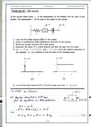
In the mechanical system of Figure 3-28, one end of the lever is connected to a spring and a damper,
and a force f ( t ) is applied to the other end of the lever. Derive a mathematical model of the
system. Assume that the displacement x is small and the lever is rigid and massless.
( ) f t
l
1
l
2
P
k
x
b
Solution
Assumptions:
1. Lever is rigid and massless.
2. Reactions at lever P are neglected.
3. Displacement x is small.
Figure 3-28
Chapter 3: Mechanical Systems 4

ME 413: System Dynamics and Control
Dr. A. Aziz Bazoune
Free Body Diagram (FBD): The FBD is shown in the Figure below
l
l
2
1
f ( t)
P
F
k
=−k x
x
Figure 3-28
F
b
= −b x&
Equation of motion:
Applying Newton’s second law, for a system in rotation about point P gives
∑
M
P
= 0 ⇒ f ( t ) l 1 − b x&
l 2 − k x l 2
=
0
DID YOU ASK YOURSELF
WHY THE RHS of the above equation is ZERO?
Rearranging, one can write:
or
( ) ( & )
f t l b x k x l
1 − + 2 =
0
⎛
l1
⎞
b x&
+ k x = ⎜
⎟
f ( t )
⎝
l2
⎠
which is the mathematical model of the system. It is clear that this differential equation
represents is a first order system since it is represented by a first order ordinary differential
equation with constant coefficients. The RHS of the above differential equation is not zero.
System Response:
In the above system, the input is the force F while the output is the displacement x . We will
try to find a relationship between the input and the output.
Taking Laplace transform of both sides of the above equations provided we have zero initial
conditions gives
Chapter 3: Mechanical Systems 5

ME 413: System Dynamics and Control
Dr. A. Aziz Bazoune
where X ( s ) and ( )
⎛
l1
⎞
( b s + k ) X ( s) = ⎜
⎟
F ( s)
⎝
l2
⎠
F s are Laplace transform of x and f ( t ) , respectively. The above
equation can be written as
Output X ( s)
⎛
l ⎞
1 C
G ( s)
= = = =
Input F s l b s k b s k
where C ( l1 l2
)
where C *
1
⎜
⎟
( ) ⎝ 2
⎠ ( + ) ( +
)
= . The above relation can be written in the standard form as:
Output X ( s)
C b C *
G ( s)
= = = =
Input F ( s) ⎛ k 1
s
⎞ ⎛ s
⎞
⎜ + ⎟ ⎜ +
⎟
⎝ b
⎠ ⎝ τ
⎠
= C b and τ = b k
( s )
F
14243
Input
C
s +
*
( 1 τ )
144424443
Transfer Function
( )
X s
1 42443
Output
The response ( )
x t will depend on the input force f ( t ) . If f ( t ) is a step input of magnitude 1:
F s = / s and
C * 1 C * α β
X ( s ) = F ( s ) = = +
⎛ 1 ⎞ s ⎛ 1 ⎞ s ⎛ 1 ⎞
⎜ s + ⎟ ⎜ s + ⎟ ⎜ s + ⎟
⎝ τ ⎠ ⎝ τ ⎠ ⎝ τ ⎠
In this case ( ) 1
where
α =
Therefore,
and hence
1
s
s C *
⎛ 1 ⎞
⎜ s + ⎟
⎝ ⎠
τ
s = 0
⎛
⎜
1 ⎝
= τC
* and β =
s
⎛ ⎞
⎜ 1 1 ⎟
X ( s ) = τ C ⎜ − ⎟
s ⎛ 1 ⎞
s
⎜ ⎜ + ⎟
τ
⎟
⎝ ⎝ ⎠ ⎠
1 ⎞
s + ⎟ C *
τ ⎠
⎛ 1 ⎞
⎜ s + ⎟
⎝ τ ⎠ 1
s = −
τ
= − τC
*
Chapter 3: Mechanical Systems 6

ME 413: System Dynamics and Control
Dr. A. Aziz Bazoune
( )
τ
⎛
1
⎜
⎝
*
x t = C − e
⎛ 1 ⎞
− ⎜ ⎟ t
⎝ τ ⎠
⎞
⎟
⎠
Chapter 3: Mechanical Systems 7