EE545 Image Processing Course Take-Home Midterm Exam

EE545 Image Processing Course
Take-Home Midterm Exam
Starts: April 16 th , 2011, 14:00 PM, Ends: April 21 st , 2011, 09:45 AM
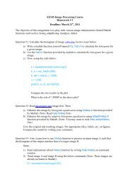
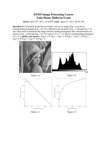
Question #1 (15 points): In the first row below you see an image (Fig. 1.a) with its
corresponding histogram (Fig. 1.b). Five different look-up tables (Fig. 1.1 through Fig. 1.5)
have been used to transform the image and the resulting histograms after transformation are
shown in Fig. 1.I through Fig. 1.V). For each LUT (1.1-1.5) find its corresponding histogram
(1.I-1.V). Justify your answer. (Fig.1.1 Fig.1.?, Fig.1.2 Fig.1.?, Fig.1.3 Fig.1.?,
Fig.1.4 Fig.1.?, Fig.1.5 Fig.1.?)
Figure 1.a Figure 1.b
Figure 1.1 Figure 1.2

Figure 1.3 Figure 1.4
Figure 1.5
Figure 1.I
Figure 1.II
Figure 1.III
Figure 1.IV

Figure 1.V
Question #2 (15 points): Describe the effect of each of the following filters. In addition,
indicate which filter will cause the most blurring and which, when convolved with a solid
(positive) intensity image, will produce the brightest image and which will produce the
darkest image. Justify your answers.
0.1 0.1 0.1 0 0 1 0 0.2 0 0 -1 0
0.1 0.1 0.1 0 -2 0 0.2 0.4 0.2 0 3 0
0.1 0.1 0.1 1 0 0 0 0.2 0 0 -1 0
(a) (b) (c) (d)
Question #3 (15 points):
a) Read image Fig2.jpg first
(http://web.iyte.edu.tr/~zubeyirunlu/teaching/ee545/Assignments/Take_Home_
Midterm_Exam/Fig2.jpg) using
x = imread ('Fig2.jpg');
and plot it. You will see that there are 9 vertical bars in the lower left of the
image. They are 6 pixels wide, 100 pixels high and the separation between
them is 19 pixels long.
b) Now, create 3 different square averaging masks of sizes 23x23, 25x25, and
45x45 and save them to h1, h2, and h3 respectively
h1=;
h2=;
h3=;
c) Then, blur image x using square averaging masks obtained in (b) and save
each result to y1, y2, and y3 respectively
y1=;
y2=;
y3=;
d) Plot each blurred image y1, y2, and y3

e) When we look at the resulting images you’ll see that the vertical bars in the
lower left of the image, in y1 and y3 are blurred, but a clear separation exists
between them. However, the bars have merged in image y2, in spite of the fact
that the kernel that produced the image is significantly smaller than the kernel
that produced image y3. Explain this.
Question #4 (10 points): The Figure 3.a and 3.b below shows an image (original) and its
corresponding frequency spectrum respectively. The following six figures (Figs. 3.1 through
3.6) displays different frequency spectrums of the original image after that some areas have
been nulled (black areas). An inverse Fourier transform of the frequency spectrums end up in
six different images (Figs. 3.I through 3.VI). For each spectrum (3.1-3.6) find its
corresponding inverse Fourier transform image (3.I-3.VI) and justify your answer. (Fig.3.1
Fig.3.?, Fig.3.2 Fig.3.?, Fig.3.3 Fig.3.?, Fig.3.4 Fig.3.?, Fig.3.5 Fig.3.?, Fig.3.6
Fig.3.?)
Figure 3.a Figure 3.b
Figure 3.1 Figure 3.2

Figure 3.3 Figure 3.4
Figure 3.5 Figure 3.6
Figure 3.I
Figure 3.II

Figure 3.III
Figure 3.IV
Figure 3.V
Figure 3.VI
Question #5 (10 points): Please answer following questions shortly but adequately.
a) In what cases is spectral (frequency domain) filtering more appropriate than
spatial one?
b) What is an “ideal low-pass filter”? Is this filter suitable to use in terms of
image processing? If yes, give an example of its application. If no, explain
why.
c) What are the common image point distance measures? Give at least two
examples and explain briefly.
Question #6 (15 points):
a) A discrete approximation of the second derivative
convolving an image I(x, y) with the kernel
1 -2 1
2
∂ I
2
∂x
can be obtained by
Use the given kernel to derive a 3 × 3 kernel that can be used to compute a discrete

approximation to the 2D Laplacian and write it below table.
Apply the Laplacian kernel to the following 3 x 3 image by convolution and fill
out the empty table below.
3 2 1
6 5 4
9 8 7
b) Why is it important to convolve an image with a Gaussian before convolving
with a Laplacian? Motivate your answer by relating to how a Laplacian filter is
defined.
c) Let us assume doing the following two operations:
1) We first convolve an image with a Gaussian and then take the Laplacian,
∇ 2 (G ∗ I)), and
2) We first apply the Laplacian to the Gaussian and then convolve the image,
(∇ 2 G) ∗ I. Will the results be the same? If yes - why? If no - why?
Question #7 (20 points): This question is about manual implementation of histogram
equalization and histogram matching (specification). Please answer the following questions.

•
•
•
•
•
•
•
•
hist.
0 0 0 0 0 0 0 0
1 1 1 1 1 1 1 1
2 2 2 2 2 2 2 2
3 3 3 3 3 3 3 3
4 4 4 4 4 4 4 4
5 5 5 5 5 5 5 5
6 6 6 6 6 6 6 6
7 7 7 7 7 7 7 7
Figure 1: 8x8(px 2 ) 3-bit assingment image.
15
14
13
12
11
10
9
8
7
6
5
4
3
2
1
0
0 1 2 3 4 5 6 7
3-bit gray levels
i 0 1 2 3
hist. 0.125 0.250 0.125 0.0312
i 4 5 6 7
hist. 0.0938 0.250 0.0938 0.0312
(a) Desired histogram plot (not normalized).
(b) Desired histogram table.
Figure 2: Desired histograms
Questions
1. Determine the possible intensity levels appearing in image of figure (1),
that is, find the gray level space of the image.
2. Find the histogram of the image shown in figure (1), and descibe histogram
as in both table form and in the stem plot form as shown in
(2(a)) and (2(b)).
3. Find the cumulative distribution function of the image of figure (1) and
use the same representations done at step (2).
4. Apply histogram equalization to image of figure (1) by using the normalized
CDF obtained at step (3) and draw the stem plot of new
histogram, is histogram changed?.

(a) Empty 8x8 image format (b) Empty 8x8 image format
for the output of histogram for the output of histogram
equalization done at step (4). matching done at step (7).
Figure 3: Empty image boxes. Use them for outputs of the specified tasks.
5. Re-scale the dynamic range of transformed image back in the range of
3-bit gray level space, namely, [0,1,2,· · · ,7] (use truncation instead of
rounding).
6. Show that histogram of figure (2(a)) and histogram of table (2(b)) are
equivalent.
7. Apply histogram specification (histogram matching) to the image of
figure (1) by using the histogram of figure (2(a)) and draw the stem
plot of new histogram. Make a comment about new histogram and
desired one.