Elliptic Curve Point Multiplication by Generalized Mersenne Numbers

JOURNAL OF ELECTRONIC SCIENCE AND TECHNOLOGY, VOL. 10, NO. 3, SEPTEMBER 2012 199
Elliptic Curve Point Multiplication by
Generalized Mersenne Numbers
Tao Wu and Li-Tian Liu
Abstract⎯Montgomery modular multiplication in
the residue number system (RNS) can be applied for
elliptic curve cryptography. In this work, unified
modular multipliers over generalized Mersenne
numbers are proposed for RNS Montgomery modular
multiplication, which enables efficient elliptic curve
point multiplication (ECPM). Meanwhile, the elliptic
curve arithmetic with ECPM is performed by mixed
coordinates and adjusted for hardware implementation.
In addition, the conversion between RNS and the binary
number system is also discussed. Compared with the
results in the literature, our hardware architecture for
ECPM demonstrates high performance. A 256-bit
ECPM in Xilinx XC2VP100 field programmable gate
array device (FPGA) can be performed in 1.44 ms,
costing 22147 slices, 45 dedicated multipliers, and 8.25K
bits of random access memories (RAMs).
Index Terms⎯Elliptic curve cryptography,
generalized Mersenne numbers, modular multiplier,
residue number system.
1. Introduction
Public key cryptography plays a significant role in
information security that it provides convenient digital
signatures and exchange of private keys [1] . Among kinds of
public key cryptography schemes, RSA cryptography [2] ,
Diffie-Hellman key exchange protocol [3] , and elliptic curve
cryptography (ECC) [4] are the most frequently used.
Especially, ECC utilizes much shorter keys to reach the
same security level as that of RSA cryptography. For
example, the ECC with a 256-bit key provides the same
security level as that of an RSA cryptosystem with a
3072-bit key [5] .
In the above cryptosystems, the fundamental operation
refers to multi-precision modular arithmetic. In RSA
Manuscript received June 25, 2012; revised July 27, 2012. This work
was partially supported by the National Natural Science Foundation of
China under Grant No. 61073173.
T. Wu and L.-T. Liu are with Department of Microelectronics and
Nanoelectronics, Tsinghua University, Beijing (e-mail: t-wu03@whu.
edu.cn; liulitian@tsinghua.edu.cn )
Digital Object Identifier: 10.3969/j.issn.1674-862X.2012.03.003
cryptography and the Diffie-Hellman key exchange
protocol, modular exponentiation is the dominant operation
in the whole computation. Within ECC the main
computation is also modular multiplication in finite field.
For instance, in the ECC digital signature protocol, there is
1 elliptic curve point multiplication (ECPM) to generate an
ECC digital signature, and 2 ECPMs to authenticate a
digital signature [5] . Meanwhile, 1 ECPM include about 10N
to 30N modular multiplication, where N is the field bit
length.
As long as ECPM over prime fields is concerned,
several designs have been implemented by setting up a
long-precision modular multiplier. With the large modular
multiplier, all modular multiplication in ECC are then
processed sequentially. In order to decrease the complexity
in arithmetic and accelerate the computation, architectures
with superior parallelism are effective and welcome. A
large Montgomery modular multiplier has been developed
with a quotient pipeline architecture [6] , and has also been
devised by a systolic array architecture [7] .
Meanwhile, in a residue number system (RNS) [8],[9]
multiprecision multiplication and addition are partitioned
into a number of single-precision operations. Such
architectures rely on the RNS Montgomery modular
multiplication algorithm [10]−[17] . A Cox-Row architecture is
built up [12] to perform modular exponentiation in RSA
cryptography, and is applied for ECPM [13] . A very large
scale integration circuit (VLSI) architecture for RNS
Montgomery modular multiplication is also proposed [18] , in
which the conversion between the binary number system
and RNS is emphasized and improved. Implementation
over other platforms like microprocessors and graphic
processing units (GPUs) have also been reported [19],[20] .
In this paper, based on RNS Montgomery modular
multiplication and generalized Mersenne numbers, an
optimized ECPM architecture is proposed for hardware
implementation. Firstly, a unified modular multiplier over
generalized Mersenne numbers is devised, which performs
modular multiplication with respect to two conjugated
moduli. A group of such modular multipliers then cover
two groups of RNS moduli, so it can be applied to RNS
Montgomery modular multiplication. Besides, the
binary-to-RNS and RNS-to-binary conversions can also be

200
carried out by configuring the RNS Montgomery modular
multiplier in different modes. Together with lots of
precomputation for RNS Montgomery modular
multiplication and mixed coordinates for ECPM,
high-performance ECPM can be carried out by efficient
modular arithmetic over generalized Mersenne numbers.
The remaining parts of this paper are organized as
follows. Section 2 introduces the background for the RNS
Montgomery modular multiplication algorithm and elliptic
curve arithmetic with ECC. Then a unified modular
multiplier is proposed for RNS Montgomery modular
multiplication in Section 3, in which the residue arithmetic
by generalized Mersenne numbers is developed. Section 4
discusses ECPM based on such RNS arithmetic, where the
RNS-to-binary conversion and its inverse operation are also
discussed. In Section 5, we give the results with hardware
implementation of ECPM over prime field. The last Section
concludes this paper.
2. Background for RNS and ECC
2.1 Residue Number System
A set of pairwise prime numbers define a residue
number system, which is called RNS moduli. Suppose RNS
Ω is defined by the moduli {m 1 , m 2 , ⋅⋅⋅, m n }, then the
dynamic range of Ω is M=∏m i for 1≤i≤n, where n is the
number of moduli. If an integer lies between the range, i.e.,
X ∈[0, M − 1] , it can then be denoted in RNS by an n-tuple:
X x1 x2
x n
Y y1 y2
y n
= ( , , , ), with x = X mod m (1 ≤i ≤ n). Set
i
= ( , , , ), then addition and multiplication can be
carried out as follows if X+Y and XY are within the
dynamic range [0, M−1]:
( 1 1
,
2 2
, ,
m n n )
1 m2
mn
= ( 1 1
,
2 2
, ,
m m n n m ).
X + Y = x + y x + y x + y
XY x y x y x y
1 2
It can be found out that the addition and multiplication
in RNS are carry-free and enjoy high parallelism.
2.2 Improved Chinese Remainder Theorem
The Chinese remainder theorem is a mathematical
connection between the binary expression and the RNS
form of a number. Suppose R=(r 1 , r 2 , ⋅⋅⋅, r n ) in Ω: {m 1 , m 2 ,
⋅⋅⋅, m n }, with M=∏m i , and M i =M/m i , for i=1, 2, ⋅⋅⋅, n. Then
the Chinese remainder theorem declares that
n
−1
i=
1 i i i
mod .
mi
R = ∑ M rM M
(1)
The improved Chinese remainder theorem replaces the
last modular reduction by subtraction [21] , i.e.,
R = ∑ M rM −α
M
(2)
n
i=
1
−1
i i i
mi
JOURNAL OF ELECTRONIC SCIENCE AND TECHNOLOGY, VOL. 10, NO. 3, SEPTEMBER 2012
i
n
whereα is an integer between [0, n−1].
−1
Denote σ = rM , then
i i i
mi
n
R = ∑ i=
1Miσ
i
−α
M
(3)
which can be rewritten as [11]
( σ )
Because 0≤R=M=(1, 1, 1). Suppose
i
x = 7 = (1, 1, 2) , then < >= (1, 1, 2) , α =
⎢⎣ 12+ 13+ 25⎥⎦ = 1, thus from (3) we have x=1×15+1×10+
2×6−1×30≡7, which is just the original number.
2.3 Modular Arithmetic in RNS
It is well-known that RNS can be used to accelerate
classic arithmetic by parallel operations, in which
short-precision modular arithmetic is employed to achieve
long-precision addition, subtraction, and multiplication. In
fact, long-precision modular addition, modular subtraction,
and modular multiplication can also be performed in RNS.
Assume A and B are two integers represented in RNS Ω,
i.e., A = ( a1, a2, , a n
) and B = ( b1, b2, , b n
), while the
moduli is {m 1 , m 2 , ⋅⋅⋅, m n } and the RNS dynamic range is M.
Suppose we have to compute the modular addition C≡A+B
(mod P) in Ω, then a pure addition C'=A+B is performed
instead of C as long as A+B

WU et al.: Elliptic Curve Point Multiplication by Generalized Mersenne Numbers 201
( a − b ) mod m by a − b + ep )modm
.
i i i
( i i i
i
2.3 RNS Montgomery Modular Multiplication
Algorithm 1. RNS Montgomery modular multiplication
Input: RNS Ω is defined by moduli {m 1 , m 2 , ⋅⋅⋅, m n },
M=∏m i , M i =M/m i , for i=1, 2, ⋅⋅⋅, n. RNS Γ is defined by
moduli {m n+1 , m n+2 , ⋅⋅⋅, m 2n }, N=∏m n+i , N i =N/m n+i , for i=1,
2, ⋅⋅⋅, n. Meanwhile, X = ( x1, x2, , xn, , x2n)
, Y = ( y1
,
y2, , yn, , y2n)
, P = ( p1, p2, , pn, , p2n)
. X·Y =< M
1 mod m >,
−
< η > =< M
1 mod m >, < ω > =< N mod m > ,
i i i
j
j j j
−
< ζ > =< N
1 mod m >, < μ > =< M mod m > ,
j j j
() i
< λ > =< Nmod
m >, < M > =< M mod m >,
i
< N > =< N mod m > ,
() i
i j i
i
j
j i j
< θ >=< η > ⋅ < − p > ,
−1
i i i
() i
() i
< χ
j
>=< M
j
pjτ jζ
j
> , < ψ
j
>=< τ
jζ
j
> ,
< φj >=< μjpjτ jζ j
>=< pjζ
j
> ,
where the tickets denotes a set of modular operations.
Output: R=< ri > : = ( r1 , r2
, , rn) =< rj > : = ( rn + 1, rn + 2,
, r2
n)
=
−
X ⋅Y⋅ M
1 mod P, with 0≤R=< xi > · < yi
> ;
2: < zj >=< xj > · < yj
> ;
3: < σ
i
>=< zi >< · θi
>;
4: < uj >=< zj > · < ψ
j
> ;
⎢ n trunc( σ
i
) ⎥
5: α = ⎢ ∑ i=
1 L
2 ⎥ ;
⎣
⎦
6: < ξ
j
>=< : u
j
>;
7: for i=1 to n
() i
8: < ξ
j
>=< : ξj > + σi⋅< χ
j
>;
9: end for
10: < v
j
>= α·
< φj
> ;
11: < ξ
j
>=< : ξj > −< v
j
>;
⎢ 2n
trunc( ξi
) ⎥
12: < r i
>=< : 0> ; 13: β = ⎢∑ i= n+
1
+ 0.5
L
2
⎥;
⎣
⎦
14: for i=1 to n
( j)
15: < ri >=< : ri >+< ξ
j
>⋅< Ni
>;
16: end for
17: < ri >=< : ri >−β⋅< λi
>;
18: < rj >=< ξ
j
> · < ω
j
> ;
19: return { < ri
> , < rj
>}.
In Algorithm 1, the main computation is two base
j
j
conversions between RNS Ω and Γ. The colon before “=”
emphasizes that it is an assignment to the original variable,
trunc(x) sets the lowest (L-l) bits of “x” as zeros and “⋅”
means modular multiplication. The value of l can be
determined by RNS moduli [11] .
According to Fermat’s little theorem, if p is a prime
−1 p−
number and GCD(a, p)=1, then a ≡ a 2 (mod p)
.
Therefore, RNS modular inverse over prime fields can be
calculated by a series of RNS modular multiplication.
2.4 ECPM
An elliptic curve over the prime field F p can be defined
by the elliptic curve equation [5] :
2 3
y = x + ax+ b
(6)
where 4a 3 +27b 2 ≠0( mod p), and p is a prime number with
p>3. In the elliptic curve field, point addition, point
doubling, and point multiplication are basic operations.
In fact, an ECPM can be separated into a series of
elliptic curve point addition and point doubling. Set Q 0 =(x 0 ,
y 0 ) as a starting point on the elliptic curve, and choose k as
a binary number with k=(k l−1 ⋅⋅⋅k 1 k 0 ) 2 . As it is shown in
Algorithm 2, the ECPM kQ 0 can be performed by the
binary left-to-right method [5] .
Algorithm 2. ECPM by point addition and point
doubling
Input: Q 0 is a point in an elliptic curve over F p , and k=
(k l−1 ⋅⋅⋅k 1 k 0 ) 2 is a binary number.
Output: S l−1 =kQ 0 .
1: S0 : = Q0;
2: for i=1 to l−1
3: Si
: = 2Si
− 1
;
4: if k l−1−i =1 then
5: Si
: = Si
+ Q0
;
6: end if
7: end for
8: return S l−1 .
In the above algorithm, the addition “+” denotes point
addition, while the multiplication of 2 denotes point
doubling.
2.5 Elliptic Curve Point Doubling and Point Addition
Assuming Q 0 is the starting point with Jacobian
coordinate (X 0 , Y 0 , Z 0 ), then its affine coordinate reads [5]
x 0 =X 0 /Z 2 0 and y 0 =Y 0 /Z 3 0 . Suppose Q 1 is the doubling point
of Q 0 , and its Jacobian coordinate is (X 1 , Y 1 , Z 1 ).
Substituting x i , y i by X i , Y i , Z i , there are
⎧ X = (3 X + aZ ) −8X Y
⎪
⎨Y X aZ X Y X Y
⎪
⎩
Z1 = 2 Y0Z0.
2 4 2 2
1 0 0 0 0
2 4 2 4
1
= (3
0
+
0)(4 0 0
−
1) −8
0
(7)
In the above equations, the parameter a is just the

202
coefficient within the elliptic curve equation:
2 3
y = x + ax+ b.
For point addition of two points P 0 and P 1 , mixed
coordinates can be applied [5] . One point P 0 keeps the affine
coordinate (x 0 , y 0 ), and the other point is denoted by the
Jacobian coordinate (X 1 , Y 1 , Z 1 ). Suppose P 2 =P 0 +P 1 , and it
has the Jacobian coordinate (X 2 , Y 2 , Z 2 ), then there is [5]
3 2
⎧ X2 = ( y0Z1 −Y1)
−
⎪
2 2 2
( xZ
0 1
− X1) ( X1+
xZ
0 1
)
⎪
3 2 2
⎨Y2 = ( y0Z1 −Y1)[ X1( x0Z1 − X1) − X2]
−
⎪
2 3
⎪
Y1( x0Z1 − X1)
2
⎪ ⎩Z2 = ( x0Z1 − X1) Z1.
3. Proposed Modular Multiplier
Generalized Mersenne numbers are widely known to
facillitate modular arithemtic [22]−[24] , and in this section
unified modular arithmetic over conjugated generalized
L k
Mersenne numbers 2 − 2 ± 1 is developed. The main
idea is to find out the most common parts between two
modular multipliers respectively over 2 L −2 k −1 and 2 L −2 k +1,
which results in an area-efficient modular multiplier
architecture for hardware implementation.
3.1 New Modular Arithmetic over Generalized
Mersenne Numbers
Suppose that A and B are two binary numbers, with
T=A·B=2 L·T h, f +T l, f. Here T h, f and T l, f are the higher and
lower halves of T. In this work, we will process the two
parts of T in parallel, in order to avoid the final full addition
before modular reduction. As a result, a carry out appears
from the lower part, which is denoted as c f and processed in
together. With T l = T l, f , T h + c f = T h, f , there is
JOURNAL OF ELECTRONIC SCIENCE AND TECHNOLOGY, VOL. 10, NO. 3, SEPTEMBER 2012
(8)
T = T h 2 L + T l + c f 2 L . (9)
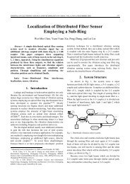
As it is shown in Fig. 1, a 54-bit multiplier can be
achieved by 18-bit multipliers, adders, and carry save logic.
Similary, other multi-precision multiplications can also be
performed by single-precision multiplications and separated
into high and low parts.
+
54 bits
54 bits
z 1
z 3
T h
×
c
B2 2 B 1 B 0
f
A 2 A 1 A 0
z2
2
z 0
T l
AAi·B i ⋅B i j
CSA
Concatenation
concatennation
72 bits
72 bits
72 bits
36 bits
72 bits
Fig. 1. L×L-bit multiplication with middle carry out bit.
Apparently, the generalized Mersenne numbers can be
divided into two kinds: m=2 L −2 k −1 and m=2 L −2 k +1. At first,
we can separately simplify the modular arithmetic with each
case.
A. m=2 L −2 k −1
Set T
1
(
1 1
)
2
2 k
h
= tL− tL− k+ tL−k
< , Th
2
= ( tL −− k 1 tt 10
) 2
<
2 L− k , then 2 L −
T k
h
= Th 1+ Th2, and
C = T mod m ≡
k
k
(2 + 1) Th + Tl + cf
(2 + 1) ≡
k L−k k
(2 + 1)(2 Th 1+ Th2) + Tl + cf
(2 + 1) ≡ (10)
L L−k k k
(2 +2 ) Th 1+ (2 + 1) Th2
+ Tl + cf
(2 + 1) ≡
L L−k k k
(2 +1+2 ) T + (2 + 1) T + T + c (2 + 1).
h1 h2
l f
Let
k L−k C′ = (2 + 2 + 1) T
k
+ (2 + 1) T + T + c
k
(2 + 1) (11)
then C′ ≡ C (mod m)
.
h1 h2
l f
k
In (11), c (2 + 1) is a (k+1)-bit number. With L−k>
f
k+1, it can be combined with 2 L − k Th
1
, i.e., 2 L − k Th
1
+
k
cf (2 + 1) = ( tL−
1tL−k 00 cf 00 cf
). Therefore,
( L−2k−1) bits ( k−1) bits
only 6 partial products need to be accumulated, all of which
are below 2 L k 2k L−1
. For example, 2 T h 1
< 2 < 2 . In the
accumulation, before final carry ripple addition, we can
employ three carry save addition to reduce the six parts to
two (L+2)-bit unsigned numbers.
Next, the bound of C' should be determined by the
modulus. It is self-evident that C ≥ 0. Meanwhile,
k L−k k k L−k
C′ (2 + 2 + 1)(2 − 1) + (2 + 1)(2 − 1) +
L k
2 − 1+ 2 + 1 =
L k 2k k+
1 k
3(2 −2 − 1) + 2 + 2 + 2 + 1 =
2k k+
1 k
3m
+ 2 + 2 + 2 + 1 <
m
2k
k+
2
3 + 2 + 2 .
(12)
L k L−1 i k L−1
i
With m = 2 −1− 2 = ∑i= 02 − 2 = ∑ i= 0, i≠k2
, k2k+2, we have
• If k=1, then L>2+2=4, i.e., L≥5. Then 2 2k + 2
k+ 2 =
5 1 1
12 2 − 2 L −
< < m .
2k k+ 2 5
• If k=2, then L>2×2+2=6. Also, 2 + 2 = 2 <
1
2 L− < m .
2k k+
2 0 i L−1
i
• If 2 + 2 .
Finally, there is always 0≤C'

WU et al.: Elliptic Curve Point Multiplication by Generalized Mersenne Numbers 203
10) 2
2 L −
tt < k , then 2 L −
T = k T
1+ T
2. Thus,
h h h
C = Tmod m≡ (2 − 1) T + T + c ⋅2
≡
(2 1)(2 ) (2 1)
(13)
(2 − 2 ) + (2 − 1) + + (2 −1)
≡
(2 1 2 ) T (2 1) T + T + c (2 −1)(mod m).
Also, set
k
L
H L f
k L−k k
− Th 1+ Th2
+ TL + cf
− ≡
L L−k k k
Th 1
Th2
Tl c
f
k L−k k k
− −
h1+ −
h2
l f
C′′ = (2 −1− 2 ) T + (2 − 1) T + T + c (2 − 1) (14)
k L−k k k
h1 h2
l f
then C′′ ≡ C (mod m)
.
k
In (14), the partial product c
f
(2 − 1) has only k bits,
and can be incorporated into 2 k T
h2
as
k
2 T + c (2 − 1) = ( t tt c c
) .
k
h2 f L−k−1 1 0
f f 2
k bits
Thus, there are also 6 partial products in accumulation, and
carry save addition can be employed to compress it to 2
parts. The upper bound of C′′ can be determined as
k k L−k k
C′′ = Tl + (2 − 1) Th2 + cf (2 −1) −(2 − 2 + 1) Th
1
≤
L k L−k k
2 − 1 + (2 −1)(2 − 1) + 2 − 1 =
L k L L−k k
(2 − 2 + 1) + (2 − 2 + 2 − 2) =
(15)
k L−2k −k
m+ m−2 (2 −1−3⋅2 ) ≤
k 2
−k
2m
−2 (2 −1−3⋅ 2 ) <
2 m.
k
As 0≤T h 1
≤ 2 − 1, the lower bound yields
L−k k L−k k k
C′′ ≥−(2 − 2 + 1) Th
1
≥ −(2 − 2 + 1)(2 − 1) =
2k k+ 1 L− k L k+ 1 L−k L
(2 − 2 ) + 2 + 1− 2 ≥ 2 + 2 + 1− 2 > (16)
k L
2 + 1− 2 > −m.
Finally, we have −m< C′′

204
A
B
REG
REG
opx
c f
0
T h
1
0
T l
1
mi
-3mi
d=2 k ±1
sign=?±1
REG
REG
0
1
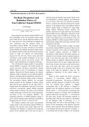
Fig. 2. Unified modular multiplier.
Register files Files
State machine
Comb
REG
CSA
i RNS1 rns1 REG
RNS-Montgomery
j RNS2 rns2 REG
modular multiplier Multiplier
i RNS1 rns1
j RNS2 rns2
-mi
JOURNAL OF ELECTRONIC SCIENCE AND TECHNOLOGY, VOL. 10, NO. 3, SEPTEMBER 2012
CSA
S
CSA
MUX
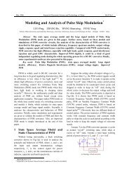
Fig. 3. ECPM based on RNS Montgomery modular multiplier.
REG
CSA
-2mi
CSA
i RNS1 rns1
j RNS2 rns2
4. ECPM by RNS Arithmetic
By RNS Montgomery modular multiplication, ECC can
be performed through RNS arithmetic. Obviously, there are
two levels of operations: 1) the modulo p operation at a
high level and 2) the modulo m i operation at a low level.
The integer p is the characteristic of the elliptic curve field,
while {m 1 , m 2 , ⋅⋅⋅, m n } are RNS moduli. In fact, the
implementation of ECC in RNS is just to replace modular
arithmetic over p by modular arithmetic over m i .
It may be doubted that there is a conflict between the
RNS Montgomery algorithm and conversion of
−
X = X ⋅M ⋅ M 1 mod p, because M is represented as zero in
RNS. Such a problem can be avoided by setting
1
X = X ⋅( M mod p) ⋅ M − mod p.
An ECPM based on RNS Montgomery modular
multiplication is illustrated in Fig. 3. In addition to the RNS
Montgomery modular multiplier, two groups of modular
CSA
CSA
i RNS1 rns1
j RNS2 rns2
adders/subtractors are employed to deal with other
operations in ECPM. The conversion from the binary
number system to RNS and the inverse operation are
considered in Section 4.1.
In particular, we have applied the left-to-right
signed-digit coding technique [25] in Algorithm 2.
4.1 Conversion between Binary Number System and
RNS
In this work, to perform binary-to-RNS conversion, e.g.,
A mod m i for i=1, 2, ⋅⋅⋅, n, a serial modular reduction
method is developed, as shown in Algorithm 4. It requires
(n−1) sequential steps to reduce an n-word integer.
Algorithm 4. Serial modular reduction
( n−1) ( n−2) (0)
Input: A= ( A A A ) L ,0≤A (i) .
It is obvious that D 0 = r 1 = R mod 2 L , and the following
process can be done by similar steps. Assume D i−1 to D 0
have been obtained, and R 0 has become
( i 1) ( i 1) ( i 1)
R = − −
i 1
( r1 , r2
, −
−
, rn
) , then
R =< r >= < r − D >⋅< > < m > (18)
() i
( i−1)
i
:
j
(
j i−1
γ
j
)mod
j
−L
where j=1, 2, ⋅⋅⋅, n. Obviously, Ri
M < 2 1. Then, by
the improved Chinese remainder theorem we have
n () i −1 () i
i
=
j=
1 i j j
−α
m j
2
R ∑ M r M M (19)
() i ⎢ n 1 () 1
where
1 trunc
i − ⎥
α =
⎛
j
r
L j
M
⎞
⎢∑ = ⎜ j ⎟+
0.5
2 ⎝
m ⎥ . Thus,
⎣
j ⎠ ⎦
−
with the precomputation of M
1 j
mod m
j
, M i mod 2 L , and
(−M) mod 2 L , (19) can be used to obtain D i =R i mod 2 L . The
accumulation in the equation can be performed by n times
of full L-bit addition. The above processes can be carried
out until R n−1 and D n−1 are obtained.

WU et al.: Elliptic Curve Point Multiplication by Generalized Mersenne Numbers 205
4.2 Moduli Selection
In the RNS Montgomery modular multiplication
algorithm, 2n RNS moduli are required by Algorithm 1.
Suppose the moduli are denoted as m ( )
k
= f1 k =
L k
2 −2 − 1 and ( ) 2 L
2 k
m 1
n+ k= f2 k = − + , with k ∈ [1,
L/2) being a set of numbers {k 1 , k 2 , ⋅⋅⋅, k n }. It is necessary
that k i (i=1, 2, …, n) make all { m
k i
} and { m
n + k i
}
pairwise prime. Except the generalized Mersenne numbers,
two special moduli 2 L and 2 L −1 are included as RNS
moduli.
For FPGA implementation, the binary length L should
be sufficiently large for coprime moduli and the RNS
dynamic range. And it is also set to be around multiples of
18, so as to use the dedicated multipliers in FPGA devices.
The seeking of moduli can be done with Wolfram
Mathematica. In this work, the RNS moduli for 192-bit,
256-bit, and 384-bit ECC over prime fields are
demonstrated in Table 1.
In Table 1, RNS 1 is the original RNS, and RNS 2 is the
auxiliary RNS. Modular multiplication over the two moduli
m i and m n+i (n=5, 6, 8) are incorporated into one unified
modular multiplier.
Table 1: RNS moduli for prime ECC
Design RNS Moduli
192-bit
ECC
256-bit
ECC
384-bit
ECC
RNS 1
RNS 2
RNS 1
RNS2
RNS1
RNS2
36
m = 2 − 1
1
36 6
m = 2 −2 − 1
3
36 12
m = 2 −2 − 1
5
36
m = 2
7
36 6
m = 2 − 2 + 1
9
36 12
m = 2 − 2 + 1
11
54
m = 2 − 1
1
54 6
m = 2 −2 − 1
3
36 2
m = 2 −2 − 1
2
36 8
m = 2 −2 − 1
4
36 14
m = 2 −2 − 1
6
36 2
m = 2 − 2 + 1
8
36 8
m = 2 − 2 + 1
10
36 14
m = 2 − 2 + 1
12
54 2
m = 2 −2 − 1
2
54 8
m = 2 −2 − 1
4
54
m = 2
5
14
−2 − 1
/
54
m = 2
6
54 6
m = 2 − 2 + 1
8
54 2
m = 2 − 2 + 1
7
54 8
m = 2 − 2 + 1
9
54
m = 2
10
14
− 2 + 1
/
54
m = 2 − 1
1
54 4
m = 2 −2 − 1
3
54 10
m = 2 −2 − 1
5
54 18
m = 2 −2 − 1
7
54
m = 2
9
54 4
m = 2 − 2 + 1
11
54 10
m = 2 − 2 + 1
13
54 18
m = 2 − 2 + 1
15
54 2
m = 2 −2 − 1
2
54 8
m = 2 −2 − 1
4
54 14
m = 2 −2 − 1
6
54 20
m = 2 −2 − 1
8
54 2
m = 2 − 2 + 1
10
54 8
m = 2 − 2 + 1
12
54 14
m = 2 − 2 + 1
14
54 20
m = 2 − 2 + 1
16
4.3 Optimized Elliptic Curve Arithmetic
The point addition and doubling in Section 2 have been
reorganized to facilitate hardware implementation [26] , which
are shown in Algorithm 5 and Algorithm 6. The basic idea
is to reduce both the computational steps and buffering
registers. The time complexity of one ECPM in this work is
T total =h·c·N·T gmult , where h is a factor determined by ECC
arithmetic, c is the number of sequential steps to finish one
RNS Montgomery modular multiplication, N is the binary
length of ECC field bits, and T gmult is the time of one
modular multiplication over generalized Mersenne numbers.
In this work, h=15 is for the average case, and h=11 is for
the best case. T gmult is just the critical path of the second
stage in Fig. 2.
In fact, the lazy RNS modular reduction [27]−[29] can be
applied to accelerate the ECPM to some extent [13],[29] . On
average, to process one ECC bit, the average number of
RNS modular reductions in this work is 11+12×1/3=15,
where the factor 1/3 is due to signed-digit coding [25] . By
contrast, only 13 sequential RNS modular reductions are
needed by the lazy RNS reduction [13],[29] . However, this
selection of ECC arithmetic steps does not affect the
efficiency of unified modular multiplier.
Algorithm 5. Optimized point doubling
Input: Point Q 0 with Jacobian coordinate (X 0 , Y 0 , Z 0 )
lies at an elliptic curve, which is defined by
2 3
y = x + ax+ b.
Output: Q 1 =2Q 0 with Q 1 = (X 1 , Y 1 , Z 1 ).
2
1: V1 = X0
, F = Y0 + Y0;
2
2: V2 = Z0
, G1 = 3⋅ V1 = V1+ V1+ V1;
2
3: V3 = V2
;
V = aV ;
4:
4 3
2
5: E = G1 + V4,
G2
= F ;
6: G3 = G2⋅ X0;
2
7: V5 = G3 + G3,
V6
= E ;
8: X1 = V6 − V5, V7 = F⋅ G2;
9: V8 = G3 − X1, G4 = V7 ⋅ Y0;
10: V9 = E⋅ V8;
11: Y1 = V9 − G4
, Z1 = Z0⋅ F ;
12: return (X 1 , Y 1 , Z 1 ).
At Line 4 of Algorithm 5, the constant a has been
represented in RNS as (a·M) mod p by precomputation,
where M is the RNS dynamic range.
Algorithm 6. Optimized point addition
Input: Point P 0 is denoted by the affine coordinate (x 0 ,
y 0 ), and the other point P 1 is denoted as a Jacobian
coordinate (X 1 , Y 1 , Z 1 ).
Output: P 2 =P 0 +P 1 with a Jacobian coordinate (X 2 , Y 2 ,
Z 2 ).

206
JOURNAL OF ELECTRONIC SCIENCE AND TECHNOLOGY, VOL. 10, NO. 3, SEPTEMBER 2012
Table 2: Hardware implementation of F p ECPM
References Prime Field Technology Max. frequency
(MHz)
Area
(Slices)
ROM+RAM
(bits)
Multipliers/DSP ECPM time
(ms)
This work 192-bit F p Xilinx XC2VP100 79.3 17747 32×192 24 1.13
This work 256-bit F p Xilinx XC2VP100 73.5 22147 (32+2) ×256 45 1.44
This work 256-bit F p Xilinx XC4VLX80 100 21572 (32+2) ×256 45 1.06
This work 384-bit F p Xilinx
99.0 35109 (32+2) ×384 72 2.03
XC4VLX160
This work 256-bit F p TSMC CMOS 0.18 123.46 221K gates (32+2) ×256 0 0.857
um process
This work 384-bit F p TSMC CMOS 0.18 123.46 324K gates (32+2) ×384 0 1.63
um process
Ref. [30] 192-bit F p Xilinx XCV1000E 52.9 25012 LUTs 0 0 2.97
Ref. [30] 256-bit F p Xilinx XCV1000E 39.7 32716 LUTs 0 0 3.95
Ref. [13] 192-bit F p Altera
89.6 12480 LE Unspecified 80 DSP 0.72
EP1S30F780C5
Ref. [13] 256-bit F p Altera
90.7 16200 LE Unspecified 125 DSP 1.17
EP1S60F780C5
Ref. [13] 256-bit F p Altera
157.2 9177 ALM Unspecified 96 DSP 0.68
EP2S30F484C3
Ref. [13] 384-bit F p Altera
150.9 12958 ALM Unspecified 177 DSP 1.35
EP2S30F484C3
Ref. [6] 192-bit F p Xilinx XCV1000E 40 11416 LUTs 35 BRAMs 0 3
Ref. [31] NIST-256 F p Xilinx XC4VSX55 375 24574 176 BRAMs 512 DSP 0.0405
Ref. [31] NIST-256 F p Xilinx XC4VSX55 490 1715 176 BRAMs 32 DSP 0.495
Ref. [32] 256-bit F p Xilinx XC2VP125 39.46 15755 0 256 3.86
2
1: H1 = Z1
;
2: H2 = x0⋅ H1;
3: S = H2 − X1, U1 = H1⋅ Z1;
4: W = H2 + X1, U2 = y0⋅ U1;
5: T = U2 − Y1,
6: H4 = H3⋅ W ;
7:
U3
2
= T ;
H3
2
= S ;
8: X
2
= U3 − H4, U4 = X1⋅ H3;
9: U5 = U4 − X2
, H5 = H3⋅ S ;
10: H6 = T⋅ U5;
11: U6 = Y1⋅ H5;
12: Y2 = H6 − U6, Z2 = S⋅ Z1;
13: return (X 2 , Y 2 , Z 2 ).
In Algorithm 5 and Algorithm 6, U i (i=1, 2, ⋅⋅⋅, 6) and V i
(i=1, 2, ⋅⋅⋅, 9) can be buffered by output registers of RNS
processing units, while the other variables need extra
registers for buffering.
5. Hardware Implementation
In this work, ECPM has been described by verilog
hardware description language (VHDL) and then
synthesized in Xilinx ISE foundation by Synplify 9.6.2.
The palce and route process is completed in Xilinx ISE
10.1. The target devices are Xilinx XC2VP100-6 FF1696
FPGA (130 nm CMOS node) and XC4VLX80-12 FF1148
FPGA (90 nm CMOS node), which can be compared with
Altera Stratix and Stratix II devices. This work is aiming at
ECPM over general prime fields. The hardware
implementation results are shown in Table 2. In order to
measure the total area complexity, we have also synthesized
the 256-bit and 384-bit F p ECPM by TSMC 0.18 μm
CMOS process, which respectively costs an area of 221K
gates (NAND2) and 324 K gates at 123.46 MHz.
The number of sequential steps c in one RNS
Montgomery modular multiplication is interfered with
hardware implementation. In this work, c=26 for 192-bit
ECC, c=24 for 256-bit ECC, and c=30 for 384-bit ECC.
Correspondingly, the number of clock cylces for each
ECPM is respectively 89984, 105785, and 201143.
Reference [30] is a pioneer for implementing F p ECPM
by RNS, in which the RNS parallelism of addition and
multiplication were exploited. However, it deals with
modular arithmetic out of RNS and therefore conversions
into and out of the binary system become a bottleneck. In
order to improve the performance, a pipelined conversion
logic unit is designed, and the multiplication in their
architecture appears in port conversions between RNS and
the binary number system. Compared with their work, the
proposed work obtains higher performance by more
hardware resources.
In Ref. [13], an efficient RNS architecture with a deep
pipeline was proposed for ECPM. It also depends on the
RNS Montgomery modular multiplication algorithm, and
the moduli are just generalized Mersenne numbers of 2 L −δ.
Its critical path is reduced owing to deep pipeline stages. In
Table 2, the Altera logic elements (LE) are equivalent to
the look-up table (LUT) of the Xilinx Virtex II-pro.
Meanwhile, one Altera DSP (digital signal processing)

WU et al.: Elliptic Curve Point Multiplication by Generalized Mersenne Numbers 207
block accounts for a 9×9-bit multiplier, while one DSP
block in Xilinx FPGA includes an 18×18-bit multiplier. In
general, this work is inferior to [13] in performance due to
only 2 pipeline stages and the relative deficiency of elliptic
curve arithmetic with ECPM.
Reference [6] is the initial work for implementing
ECPM in FPGA, in which a high-radix Montgomery
modular multiplier was used to perform ECPM, which is
very area-efficient but relatively slow compared with other
designs.
In [31], ECPM architectures for NIST (American
National Institute of Standards and Technology) prime
fields were implemented in FPGA. It makes best use of
FPGA DSP resources to achieve a very high frequency,
which is quite fast compared with both hardware and
software implementation in the literature. However, the
high frequency may be unavailable in many applications.
Also it depends heavily on the special DSP units and is
only applicable to NIST primes.
The work in [32] focused on the improvement of
modular inverse in the elliptic curve field, which brings out
good performance compared with related designs. In detail,
in Xilinx XC2VP125-9 FPGA it requires 15755 slices and
256 18×18-bit multipliers for a 256-bit Fp ECPM, and
computes one ECPM by 3.86 ms. By contrast, our work in
Xilinx XC2VP100-8 FPGA requires 22147 slices and 45
18×18-bit multipliers, and completes one ECPM in 1.44 ms.
Apparently, the proposed design enjoys better performance
than [32].
6. Conclusions
In this work, we have improved the modular arithmetic
over generalized Mersenne numbers m=2 L −2 k ±1, by which
a unified modular multiplier working over this pair of
numbers can be obtained. Modular reductions over such
generalized Mersenne numbers can be performed by a little
addition and a few multiplexors.
This modular multiplier is then applied for ECPM by
the RNS Montgomery modular multiplication algorithm.
Together with the partially optimized point addition and
doubling for elliptic curve arithmetic, the proposed ECPM
demonstrates good performance for hardware
implementation in FPGA and application specific integrated
circuits (ASIC).
Acknowledgment
The authors would like to thank the comments from
anonymous reviewers. Discussion with Prof. Shuguo Li is also
acknowledged.
References
[1] A. J. Menezes, P. C. van Oorschot, and S. A. Vanstone,
Handbook of Applied Cryptography, Boca Raton: CRC
Press, 1997.
[2] R. Rivest, A. Shamir, and L. Adleman, “A method for
obtaining digital signatures and public-key cryptosystems,”
Communications of the ACM, vol. 21, no. 2, pp. 120–126,
1978.
[3] W. Diffie and M. E. Hellman, “New directions in
cryptography,” IEEE Trans. on Information Theory, vol.
IT-22, pp. 644–654, Nov. 1976.
[4] N. Koblitz, “Elliptic curve cryptosystems,” Mathematics of
Computation, vol. 48, pp. 203–209, 1987, doi:
http://dx.doi.org/10.1090/S0025-5718-1987-0866109-5
[5] D. Hankerson, A. Menezes, and S. Vanstone, Guide to
Elliptic Curve Cryptography, New York: Springer-Verlag,
2004.
[6] G. Orlando and C. Paar, “A scalableGF(p) elliptic curve
processor architecture for programmable hardware,” in Proc.
of the 3rd Int. Workshop on Cryptographic Hardware and
Embedded Systems, Paris, 2001, pp. 348–363.
[7] S. Örs, L. Batina, and B. Preneel, “Hardware
implementation of elliptic curve processor over GF(p),” in
Proc. of IEEE Int. Conf. on Application-Specific Systems,
Architectures, and Processors, Hague, 2003, pp. 433–443.
[8] P. Mohan, Residue Number Systems: Algorithms and
Architectures, Boston: Kluwer Academic Publishers, 2002.
[9] M. Soderstrand, W. Jenkins, G. Jullien, and F. Taylor,
Residue Number System Arithmetic: Modern Applications in
Signal Processing, New York: IEEE Press, 1986.
[10] K. Posch and R. Posch, “Modulo reduction in residue
number system,” IEEE Trans. on Parrallel and Distributed
Systems, vol. 6, no. 5, pp. 449–454, 1995.
[11] S. Kawamura, M. Koike, F. Sano, and A. Shimbo,
“Cox-rower architecture for fast parallel montgomery
multiplication,” in Proc. of Advances in Cryptology-
EUROCRYPT 2000, Bruges, 2000, pp. 523–538.
[12] H. Nozaki, M. Motoyama, A. Shimbo, and S. Kawamura,
“Implementation of rsa algorithm based on rns montgomery
modular multiplication,” in Proc. of the 3rd Int. Workshop
on Cryptographic Hardware and Embedded Systems, Paris,
2001, pp. 364–376.
[13] N. Guillermin, “A high speed coprocessor for elliptic curve
scalar multiplications over F p ,” in Proc. of Cryptographic
Hardware and Embedded Systems 2010, Santa Barbara,
2010, pp. 48–64.
[14] Z. Lim and B. Phillips, “An rns-enhanced microprocessor
implementation of public key cryptography,” in Proc. of the
41st Asilomar Conf. on Signals, Systems and Computers,
Pacific Grove, 2007, pp. 1430–1434.
[15] J. Bajard, L. Didier, and P. Kornerup, “An RNS
montgomery modular multiplication algorithm,” IEEE Trans.
on Computers, vol. 47, no. 7, pp. 766–776, 1998.
[16] J. Bajard, L. Didier, and P. Kornerup, “Modular
multiplication and base extensions in residue number
systems,” in Proc. of the 15th IEEE Symposium on
Computer Arithmetic, Vail, 2001, pp. 59–65.
[17] J. Bajard and L. Imbert, “A full RNS implementation of
RSA,” IEEE Tran. on Computers, vol. 53, no. 6, pp.
769–774, 2004.
[18] D. Schinianakis and T. Stouraitis, “A rns montgomery
multiplication architecture,” in Proc. of IEEE Symposium on
Circuits and Systems, Rio de Janeiro, 2011, pp. 1167–1171.

208
JOURNAL OF ELECTRONIC SCIENCE AND TECHNOLOGY, VOL. 10, NO. 3, SEPTEMBER 2012
[19] Z. Lim, B. Phillips, and M. Liebelt, “Elliptic curve digital
signature algorithm over g f (p) on a residue number system
enabled microprocessor,” in Proc. of IEEE Region 10 Conf.,
TENCON, Singapore, 2009, pp. 1–6.
[20] S. Antão, J. Bajard, and L. Sousa, “Elliptic curve point
multiplication on gpus,” in Proc. of the 21st IEEE Int. Conf.
on Application-Specific Systems, Architectures and
Processors, Rennes, 2010, pp. 192–199.
[21] A. Shenoy and R. Kumaresan, “Fast base extension using a
redundant modulus in rns,” IEEE Trans. on Computers, vol.
38, no. 2, pp. 292–297, 1989.
[22] A. Hiasat, “New efficient structure for a modular multiplier
for RNS,” IEEE Trans. on Computers, vol. 49, no. 2, pp.
170–174, 2000.
[23] M. Ciet, M. Neve, E. Peeters, and J.-J. Quisquater, “Parallel
FPGA implementation of RSA with residue number systems
—can sidechannel threats be avoided?” in Porc. of the 46th
IEEE Int. Midwest Symposium on Circuits and Systems,
Cairo, 2003, pp. 806–810.
[24] J. Bajard, M. Kaihara, and T. Plantard, “Selected rns bases
for modular multiplication,” in Porc. of the 19th IEEE
Symposium on Computer Arithmetic, 2009, pp. 25–32.
[25] M. Joye and S. Yen, “Optimal left-to-right binary
signed-digit recoding,” IEEE Trans. on Computers, vol. 49,
no. 7, pp. 740–748, 2000.
[26] M. Brown, D. Hankerson, J. López, and A. Menezes,
“Software implementation of the NIST elliptic curves over
prime fields,” in Proc. of Topics in Cryptology-CT-RSA
2001, San Francisco, 2001, pp. 250–265.
[27] R.-C. Cheung, S. Duquesne, J. Fan, N. Guillermin, I.
Verbauwhede, and G.-X. Yao, “FPGA implementation of
pairings using residue number system and lazy reduction,”
in Proc. of Cryptographic Hardware and Embedded Systems,
Nara, 2011, pp. 421–441.
[28] J. Bajard, L. Imbert, P. Liardet, and T. Yannick, “Leak
resistant arithmetic,” in Proc. of Cryptographic Hardware
and Embedded Systems, Cambridge, 2004, pp. 62–75.
[29] J. Bajard, S. Duquesne, and M. Ercegovac, Combining
Leakresistant Arithmetic for Elliptic Curves Defined over F p
and RNS Representation. [Online]. Available: http://eprint.
iacr.org
[30] D. Schinianakis, A. Fournaris, H. M. A. Kakarountas, and T.
Stouraitis, “An rns implementation of an Fp elliptic curve
point multiplier,” IEEE Trans. on Circuits and Systems, I:
Regular Papers, vol. 56, no. 6, pp. 1202–1213, 2009.
[31] T. Güneysu and C. Paar, “Ultra high performance ecc over
NIST primes on commercial FPGAs,” in Proc. of Int.
Workshop on Cryptographic Hardware and Embedded
Software, Washington, D.C., 2008, pp. 62–78.
[32] C. McIvor, M. McLoone, and J.V.McCanny, “Hardware
elliptic curve cryptographic processor over GF(p),” IEEE
Trans. on Circuits and Systems, I: Regular Papers, vol. 53,
no. 9, pp. 1946–1957, 2006.
Tao Wu was born in 1981 in Hubei Province.
He received the B.S. degree in electronic
science and technology from Wuhan
University, Wuhan in 2003 and the M.S.
degree from Tsinghua University, Beijing in
2006. From September 2006 to April 2007, he
served as a temporary assistant with the
Device and System Laboratory, the
Institute of Micro-electronics, Tsinghua University. Then he
worked with the Department of Physics and Electronic
Engineering, Guangxi Normal University from July 2007 to July
2008 . Since September 2008 he has been pursuing the Ph.D.
degree with Tsinghua University. His current research refers to
circuits and computer arithmetic about public-key cryptography.
Li-Tian Liu was born in 1947 in Jiangxi
Province. He received the B.S. degree in
electronic engineering from Tsinghua
University, Beijing in 1970. He is currently a
full professor with the Institute of
Microelectronics, Tsinghua University. His
research interests include the development of
semiconductor devices and integrated circuits.