Data Mining Algorithms - Quretec

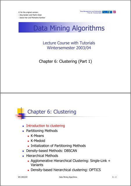
© for the original version: 

-JörgSander and Martin Ester 

- Jiawei Han and Micheline Kamber 

Data Management and Exploration 

Prof. Dr. Thomas Seidl 

Data Mining Algorithms 

Lecture Course with Tutorials 

Wintersemester 2003/04 

Chapter 6: Clustering (Part 1) 

Chapter 6: Clustering 

• Introduction to clustering 

• Partitioning Methods 

• K-Means 

• K-Medoid 

• Initialization of Partitioning Methods 

• Density-based Methods: DBSCAN 

• Hierarchical Methods 

• Agglomerative Hierarchical Clustering: Single-Link + 

Variants 

• Density-based hierarchical clustering: OPTICS 

WS 2003/04 Data Mining Algorithms 6 – 2

What is Clustering? 

• Grouping a set of data objects into clusters 

• Cluster: a collection of data objects 

• Similar to one another within the same cluster 

• Dissimilar to the objects in other clusters 

• Clustering = unsupervised classification (no predefined classes) 

• Typical usage 

• As a stand-alone tool to get insight into data distribution 

• As a preprocessing step for other algorithms 

WS 2003/04 Data Mining Algorithms 6 – 3 

Measuring Similarity 

• To measure similarity, often a distance function dist is used 

• Measures “dissimilarity” between pairs objects x and y 

• Small distance dist(x, y): objects x and y are more similar 

• Large distance dist(x, y): objects x and y are less similar 

• Properties of a distance function 

• dist(x, y) ≥ 0 

• dist(x, y) = 0 iff x = y (definite) (iff = if and only if) 

• dist(x, y) = dist(y, x) (symmetry) 

• If dist is a metric, which is often the case: 

dist(x, z) ≤ dist(x, y) + dist(y, z) (triangle inequality) 

• Definition of a distance function is highly application dependent 

• May require standardization/normalization of attributes 

• Different definitions for interval-scaled, boolean, categorical, 

ordinal and ratio variables 


Example distance functions I 

• For standardized numerical attributes, i.e., vectors x = (x 1 , ..., x d ) and 

y = (y 1 , ..., y d ) from a d-dimensional vector space: 

• General L p -Metric (Minkowski-Distance): 

dist( 

x, 

y) 

= 

p 

d 

∑ 

i= 

1 

( x i 

− y i 

) 

p 

• Euclidean Distance (p = 2): 

dist( 

x, 

y) 

= 

d 

∑ 

i= 

1 

( x i 

− y i 

) 

2 

• Manhattan-Distance (p = 1): dist( 

x, 

y) 

= 

• Maximum-Metric (p = ∞): 

d 

∑ 

i= 

1 

x i 

− y i 

{ x − y , ≤ i ≤ d} 

dist( 

x, 

y) 

= max 1 

i 

i 

• For sets x and y: 

dist( 

x, 

y) 

= 

x ∪ y − x ∩ y 

x ∪ y 


Example distance functions II 

• For categorical attributes: 

d 

∑ 

= ⎩ ⎨⎧ 0 if x 

= 

= 

= i 

y 

dist( x, 

y) 

δ ( xi 

, yi 

) where δ ( xi 

, yi 

) 

i 1 1 else 

• For text documents: 

• A document D is represented by a vector r(D) of frequencies of the 

terms occuring in D, e.g., 

( f ( ti, 

D) 

), 

ti 

∈ } 

r( d) 

= {log 

T 

where f (t i , D) is the frequency of term t i in document D 

• The distance between two documents D 1 

and D 2 

is defined by the 

cosine of the angle between the two vectors x = r(D 1 

) and y = r(D 2 

): 

x, 

y 

dist( 

x, 

y) 

= 1− 

x ⋅ y 

where 〈 .,.〉is the inner product and | .|is the length of vectors 

i 


General Applications of Clustering 

• Pattern Recognition and Image Processing 

• Spatial Data Analysis 

• create thematic maps in GIS by clustering feature spaces 

• detect spatial clusters and explain them in spatial data mining 

• Economic Science (especially market research) 

• WWW 

• Documents 

• Web-logs 

• Biology 

• Clustering of gene expression data 


A Typical Application: Thematic Maps 

• Satellite images of a region in different wavelengths 

• Each point on the surface maps to a high-dimensional feature 

vector p = (x 1 , …, x d ) where x i is the recorded intensity at the 

surface point in band i. 

• Assumption: each different land-use reflects and emits light of 

different wavelengths in a characteristic way. 

(12),(17.5) • 

•••• 

••• 

•••• 

•••• •••• 

(8.5),(18.7) ••••• 

•••• 

1112 

1122 

3 2 3 2 

3333 

Surface of the earth 

Cluster 2 

Band 1 Cluster 1 

12 

• 

• 

• 

• 

• • • • 

• • 

10 • 

Cluster 3 

• • 

8 

• • 

Band 2 

16.5 18.0 20.0 22.0 

Feature-space 


Application: Web Usage Mining 

Determine Web User Groups 

Sample content of a web log file 

romblon.informatik.uni-muenchen.de lopa - [04/Mar/1997:01:44:50 +0100] "GET /~lopa/ HTTP/1.0" 200 1364 

romblon.informatik.uni-muenchen.de lopa - [04/Mar/1997:01:45:11 +0100] "GET /~lopa/x/ HTTP/1.0" 200 712 

fixer.sega.co.jp unknown - [04/Mar/1997:01:58:49 +0100] "GET /dbs/porada.html HTTP/1.0" 200 1229 

scooter.pa-x.dec.com unknown - [04/Mar/1997:02:08:23 +0100] "GET /dbs/kriegel_e.html HTTP/1.0" 200 1241 

Generation of sessions 

Session::= 

which entries form a single session? 

Distance function for sessions: 

d( x, y) 

= 

| x∪ y| −| x∩ 

y| 

| x∪ 

y| 


Major Clustering Approaches 

• Partitioning algorithms 

• Find k partitions, minimizing some objective function 

• Hierarchy algorithms 

• Create a hierarchical decomposition of the set of objects 

• Density-based 

• Find clusters based on connectivity and density functions 

• Other methods 

• Grid-based 

• Neural networks (SOM’s) 

• Graph-theoretical methods 

• . . . 





• K-Means 

• K-Medoid 





Variants 



Partitioning Algorithms: Basic Concept 

• Goal: Construct a partition of a database D of n objects into a set of k 

clusters minimizing an objective function. 

• Exhaustively enumerating all possible partitions into k sets in order 

to find the global minimum is too expensive. 

• Heuristic methods: 

• Choose k representations for clusters, e.g., randomly 

• Improve these initial representations iteratively: 

• Assign each object to the cluster it “fits best” in the current clustering 

• Compute new cluster representations based on these assignments 

• Repeat until the change in the objective function from one iteration to the 

next drops below a threshold 

• Types of cluster representations 

• k-means: Each cluster is represented by the center of the cluster 

• k-medoid: Each cluster is represented by one of its objects 

• EM: Each cluster is represented by a probability distribution 





• K-Means 

• K-Medoid 





Variants 



K-Means Clustering: Basic Idea 

• Objective: For a given k, form k groups so that the sum of the 

(squared) distances between the mean of the groups and their 

elements is minimal. 

• Poor Clustering 

5 

5 

x 

x 

x 

1 

1 

x Centroids 

1 

5 

1 

5 

• Optimal Clustering 

5 

5 

x 

x 

1 

1 

x 

x Centroids 

1 

5 

1 

5 


K-Means Clustering: Basic Notions 

• Objects p=(x p 1, ..., x p d) are points in a d-dimensional vector space 

(the mean of a set of points must be defined) 

• Centroid µ C : Mean of all points in a cluster C 

• Measure for the compactness of a cluster C: 

TD 

2 

∑ 

( C) 

= dist( 

p, 

µ ) 

p∈C 

• Measure for the compactness of a clustering 

k 

2 2 

TD = ∑ TD ( Ci) 

i= 

1 

C 

2 


K-Means Clustering: Algorithm 

Given k, the k-means algorithm is implemented in 4 steps: 

1. Partition the objects into k nonempty subsets 

2. Compute the centroids of the clusters of the 

current partition. The centroid is the center (mean 

point) of the cluster. 

3. Assign each object to the cluster with the nearest 

representative. 

4. Go back to Step 2, stop when representatives do 

not change. 


K-Means Clustering: Example 

10 

9 

8 

7 

6 

5 

4 

3 

2 

1 

0 

0 1 2 3 4 5 6 7 8 9 10 

10 

9 

8 

7 

6 

5 

4 

3 

2 

1 

0 

0 1 2 3 4 5 6 7 8 9 10 

10 

9 

8 

7 

6 

5 

4 

3 

2 

1 

0 

0 1 2 3 4 5 6 7 8 9 10 

10 

9 

8 

7 

6 

5 

4 

3 

2 

1 

0 

0 1 2 3 4 5 6 7 8 9 10 


K-Means Clustering: Discussion 

• Strength 

• Relatively efficient: O(tkn), where n is # objects, k is # clusters, 

and t is # iterations. Normally, k, t




• K-Means 

• K-Medoid 





Variants 



K-Medoid Clustering: Basic Idea 

• Objective: For a given k, find k representatives in the dataset so 

that, when assigning each object to the closest representative, the 

sum of the distances between representatives and objects which 

are assigned to them is minimal. 

Data Set 

Poor Clustering 

Optimal Clustering 

5 

5 

5 

1 

1 

Medoid 

1 

Medoid 

1 

5 

1 

5 

1 

5 


K-Medoid Clustering: Basic Notions 

• Requires arbitrary objects and a distance function 

• Medoid m C : representative object in a cluster C 

• Measure for the compactness of a Cluster C: 

∑ 

TD ( C) 

= dist( 

p, 

) 

p∈C 

m C 

• Measure for the compactness of a clustering 

TD = 

k 

∑ 

i= 

1 

TD( 

Ci 

) 


K-Medoid Clustering: PAM Algorithm 

• [Kaufman and Rousseeuw, 1990] 

• Given k, the k-medoid algorithm is implemented in 5 steps: 

1. Select k objects arbitrarily as medoids (representatives); 

assign each remaining (non-medoid) object to the cluster with 

the nearest representative, and compute TD current . 

2. For each pair (medoid M, non-medoid N) 

compute the value TD N↔M , i.e., the value of TD for the partition 

that results when “swapping” M with N 

3. Select the non-medoid N for which TD N↔M is minimal 

4. If TD N↔M is smaller than TD current 

Swap N with M 

Set TD current 

:= TD N↔M 

Go back to Step 2 

5. Stop. 


K-Medoid Clustering: CLARA and CLARANS 

• CLARA [Kaufmann and Rousseeuw,1990] 

• Additional parameter: numlocal 

• Draws numlocal samples of the data set 

• Applies PAM on each sample 

• Returns the best of these sets of medoids as output 

• CLARANS [Ng and Han, 1994) 

• Two additional parameters: maxneighbor and numlocal 

• At most maxneighbor many pairs (medoid M, non-medoid N) are 

evaluated in the algorithm. 

• The first pair (M, N) for which TD N↔M is smaller than TD current is 

swapped (instead of the pair with the minimal value of TD N↔M ) 

• Finding the local minimum with this procedure is repeated 

numlocal times. 

• Efficiency: runtime(CLARANS) < runtime(CLARA) < runtime(PAM) 


CLARANS Selection of Representatives 

CLARANS(objects DB, Integer k, Real dist, 

Integer numlocal, Integer maxneighbor) 

for r from 1 to numlocal do 

Randomly select k objects as medoids; i := 0; 

while i < maxneighbor do 

Randomly select (Medoid M, Non-medoid N); 

Compute changeOfTD_:= TD N↔M − TD; 

if changeOfTD < 0 then 

substitute M by N; 

TD := TD N↔M ; i := 0; 

else i:= i + 1; 

if TD < TD_best then 

TD_best := TD; Store current medoids; 

return Medoids; 


K-Medoid Clustering: Discussion 

• Strength 

• Applicable to arbitrary objects + distance function 

• Not so sensitive to noisy data and outliers as k-means 

• Weakness 

• Inefficient 

• Like k-means: need to specify the number of clusters k in advance, 

and clusters are forced to have convex shapes 

• Result and runtime for CLARA and CLARANS may vary largely due to 

the randomization 

TD(CLARANS) 

TD(PAM) 





• K-Means 

• K-Medoid 





Variants 



Initialization of Partitioning Clustering 

Methods 

• [Fayyad, Reina and Bradley 1998] 

• Draw m different (small) samples of the dataset 

• Cluster each sample to get m estimates for k 

representatives 

A = (A 1 , A 2 , . . ., A k ), B = (B 1 ,. . ., B k ), ..., M = (M 1 ,. . ., M k ) 

• Then, cluster the set DS = A ∪ B ∪ … ∪ M m times, 

using the sets A, B, ..., M as respective initial partitioning 

• Use the best of these m clusterings as initialization for 

the partitioning clustering of the whole dataset 


Initialization of Partitioning Clustering 

Methods 

Example 

D3 

A3 

C3 

C1 

A1 

D1 

B1 

D2 B3 

B2 

A2 

C2 

whole dataset 

k = 3 

DS 

m = 4 samples 

true cluster centers 


Choice of the Parameter k 

• Idea for a method: 

• Determine a clustering for each k = 2, ... n-1 

• Choose the „best“ clustering 

• But how can we measure the quality of a clustering? 

• A measure has to be independent of k. 

• The measures for the compactness of a clustering TD 2 and TD 

are monotonously decreasing with incresing value of k. 

• Silhouette-Coefficient [Kaufman & Rousseeuw 1990] 

• Measureforthequalityof a k-means or a k-medoid clustering 

that is independent of k. 


The Silhouette Coefficient 

• a(o): average distance between object o and the objects in its cluster A 

• b(o): average distance between object o and the objects in its “second 

closest” cluster B 

bo ( ) − ao ( ) 

• The silhouette of o is then defined as so ( ) = 

max{ ao ( ), bo ( )} 

• measures how good the assignment of o to its cluster is 

• s(o) = −1: bad, on average closer to members of B 

s(o) = 0: in-between A and B 

s(o) = 1: good assignment of o to its cluster A 

• Silhouette Coefficient s C of a clustering: average silhouette of all objects 

• 0.7 < s C ≤ 1.0 strong structure, 0.5 < s C ≤ 0.7 medium structure 

• 0.25 < s C ≤ 0.5 weak structure, s C ≤ 0.25 no structure 





• K-Means 

• K-Medoid 





Variants 



Density-Based Clustering 

• Basic Idea: 

• Clusters are dense regions in the 

data space, separated by regions 

of lower object density 

• Why Density-Based Clustering? 

Results of a k-medoid 

algorithm for k=4 

Different density-based approaches exist (see Textbook & Papers) 

Here we discuss the ideas underlying the DBSCAN algorithm 


Density Based Clustering: Basic Concept 

• Intuition for the formalization of the basic idea 

• For any point in a cluster, the local point density around that 

point has to exceed some threshold 

• The set of points from one cluster is spatially connected 

• Local point density at a point p defined by two parameters 

• ε – radius for the neighborhood of point p: 

N ε (p) := {q in data set D | dist(p, q) ≤ε} 

• MinPts – minimum number of points in the given 

neighbourhood N(p) 

• q is called a core object (or core point) 

w.r.t. ε, MinPts if | N ε (q) | ≥ MinPts 

ε 

q 

MinPts = 5 q is a core object 


Density Based Clustering: Basic 

Definitions 

p 

• p directly density-reachable from q 

w.r.t. ε, MinPts if 

1) p ∈ N ε (q) and 

2) q is a core object w.r.t. ε, MinPts 

p 

q 

• density-reachable: transitive closure 

of directly density-reachable 

q 

p 

• p is density-connected to a point q 

w.r.t. ε, MinPts if there is a point o such 

that both, p and q are density-reachable 

from o w.r.t. ε, MinPts. 

o 

q 


Density Based Clustering: Basic 

Definitions 

• Density-Based Cluster: non-empty subset S of database D satisfying: 

1) Maximality: if p is in S and q is density-reachable from p then q is in S 

2) Connectivity: each object in S is density-connected to all other objects 

• Density-Based Clustering of a database D : {S 1 , ..., S n ; N} where 

• S 1 

, ..., S n : all density-based clusters in the database D 

• N = D \{S 1 

, ..., S n } is called the noise (objects not in any cluster) 

Noise 

Border 

Core 

ε = 1.0 

MinPts = 5 


Density Based Clustering: DBSCAN 

Algorithm 

• Basic Theorem: 

• Each object in a density-based cluster C is density-reachable 

from any of its core-objects 

• Nothing else is density-reachable from core objects. 

for each o ∈ D do 

if o is not yet classified then 

if o is a core-object then 

collect all objects density-reachable from o 

and assign them to a new cluster. 

else 

assign o to NOISE 

• density-reachable objects are collected by performing 

successive ε-neighborhood queries. 


DBSCAN Algorithm: Example 

• Parameter 

• ε = 2.0 

• MinPts = 3 






else 




• Parameter 

• ε = 2.0 







else 




• Parameter 

• ε = 2.0 







else 



DBSCAN Algorithm: Performance 

• Runtime complexities 

N ε -query DBSCAN 

- without support (worst case): O(n) O(n 2 ) 

- tree-based support (e.g. R*-tree) : O(log(n)) O(n ∗ log(n) ) 

- direct access to the neighborhood: O(1) O(n) 

• Runtime Comparison: DBSCAN (+R*-tree) ↔ CLARANS 

Time (sec.) 

No. of Points 1,252 2,503 3,910 5,213 6,256 7,820 8,937 10,426 12,512 62,584 

DBSCAN 3 7 11 16 18 25 28 33 42 233 

CLARANS 758 3,026 6,845 11,745 18,029 29,826 39,265 60,540 80,638 ????? 


Determining the Parameters ε and MinPts 

• Cluster: Point density higher than specified by ε and MinPts 

• Idea: use the point density of the least dense cluster in the data 

set as parameters – but how to determine this? 

• Heuristic: look at the distances to the k-nearest neighbors 

p 

q 

3-distance(p) : 

3-distance(q) : 

• Function k-distance(p): distance from p to the its k-nearest 

neighbor 

• k-distance plot: k-distances of all objects, sorted in decreasing 

order 



• Example k-distance plot 

3-distance 

first „valley“ 

Objects 

• Heuristic method: 

• Fix a value for MinPts (default: 2 × d –1) 

„border object“ 

• User selects “border object” o from the MinPts-distance plot; 

ε is set to MinPts-distance(o) 



• Problematic example 

A 

C 

F 

E 

A, B, C 

B 

D’ 

D 

G1 

G 

G3 

G2 

3-Distance 

B, D, E 

B‘, D‘, F, G 

D1, D2, 

G1, G2, G3 

B’ D1 

D2 

Objects 


Density Based Clustering: Discussion 

• Advantages 

• Clusters can have arbitrary shape and size 

• Number of clusters is determined automatically 

• Can separate clusters from surrounding noise 

• Can be supported by spatial index structures 

• Disadvantages 

• Input parameters may be difficult to determine 

• In some situations very sensitive to input parameter 

setting 





• K-Means 

• K-Medoid 





Variants 



From Partitioning to Hierarchical 

Clustering 

• Global parameters to separate all clusters with a partitioning 

clustering method may not exist 

and/or 

hierarchical 

cluster structure 

largely differing 

densities and sizes 

‣ Need a hierarchical clustering algorithm in these situations 


Hierarchical Clustering: Basic Notions 

• Hierarchical decomposition of the data set (with respect to a given 

similarity measure) into a set of nested clusters 

• Result represented by a so called dendrogram 

• Nodes in the dendrogram represent possible clusters 

• can be constructed bottom-up (agglomerative approach) or top 

down (divisive approach) 

Step 0 Step 1 Step 2 Step 3 Step 4 

a 

b 

c 

d 

e 

a b 

d e 

a b c d e 

c d e 

Step 4 Step 3 Step 2 Step 1 Step 0 

agglomerative 

divisive 


Hierarchical Clustering: Example 

• Interpretation of the dendrogram 

5 

1 

• The root represents the whole data set 

• A leaf represents a single objects in the data set 

• An internal node represent the union of all objects in its sub-tree 

• The height of an internal node represents the distance between its 

two child nodes 

1 

1 

7 

2 4 6 

3 5 

5 

8 9 

1 2 3 4 5 6 7 8 9 

2 

1 

0 

distance 

between 

clusters 





• K-Means 

• K-Medoid 





Variants 



Agglomerative Hierarchical Clustering 

1. Initially, each object forms its own cluster 

2. Compute all pairwise distances between the initial clusters 

(objects) 

3. Merge the closest pair (A, B) in the set of the current clusters 

into a new cluster C = A ∪ B 

4. Remove A and B from the set of current clusters; insert C into 

the set of current clusters 

5. If the set of current clusters contains only C (i.e., if C 

represents all objects from the database): STOP 

6. Else: determine the distance between the new cluster C and 

all other clusters in the set of current clusters; go to step 3. 

‣ Requires a distance function for clusters (sets of objects) 


Single Link Method and Variants 

• Given: a distance function dist(p, q) for database objects 

• The following distance functions for clusters (i.e., sets of objects) X 

and Y are commonly used for hierarchical clustering: 

Single-Link: 

dist _ sl( 

X , Y ) = 

min 

x∈X 

, y∈Y 

dist( 

x, 

y) 

Complete-Link: 

dist 

_ cl( 

X , Y ) 

= 

max 

x∈X 

, y∈Y 

dist( 

x, 

y) 

Average-Link: 

dist _ al( 

X , Y ) = 

| 

X 

1 

| ⋅| 

Y 

⋅ 

| 

∑ 

x∈X 

, y∈Y 

dist( 

x, 

y) 





• K-Means 

• K-Medoid 





Variants 



Density-Based Hierarchical Clustering 

• Observation: Dense clusters are completely contained 

by less dense clusters 

C 

C 1 

C 2 

D 

• Idea: Process objects in the “right” order and keep track of point 

density in their neighborhood 

C 

MinPts = 3 

C 1 

C 2 

ε 2 ε 1 


Core- and Reachability Distance 

• Parameters: “generating” distance ε, fixed value MinPts 

• core-distance ε,MinPts (o) 

“smallest distance such that o is a core object” 

(if that distance is ≤ ε; “?” otherwise) 

MinPts = 5 

• reachability-distance ε,MinPts (p, o) 

“smallest distance such that p is 

directly density-reachable from o” 

(if that distance is ≤ ε; “?” otherwise) 

q 

p 

o 

ε 

core-distance(o) 

reachability-distance(p,o) 

reachability-distance(q,o) 


The Algorithm OPTICS 

• Basic data structure: controlList 

• Memorize shortest reachability distances seen so far 

(“distance of a jump to that point”) 

• Visit each point 

• Make always a shortest jump 

• Output: 

• order of points 

• core-distance of points 

• reachability-distance of points 


The Algorithm OPTICS 

ControlList 

≥ 

foreach o ∈ Database 

// initially, o.processed = false for all objects o 

if o.processed = false; 

insert (o, “?”) into ControlList; 

while ControlList is not empty 

database 

select first element (o, r-dist) from ControlList; 

retrieve N ε 

(o) and determine c_dist= core-distance(o); 

set o.processed = true; 

write (o, r_dist, c_dist) to file; 

if o is a core object at any distance ≤ ε 

foreach p ∈ N ε 

(o) not yet processed; 

determine r_dist p 

= reachability-distance(p, o); 

if (p, _) ∉ ControlList 

insert (p, r_dist p 

) in ControlList; 

else if (p, old_r_dist) ∈ ControlList and r_dist p 

< old_r_dist 

update (p, r_dist p 

) in ControlList; 

ControlList ordered by 

reachability-distance. 

cluster-ordered 

file 


OPTICS: Properties 

• “Flat” density-based clusters wrt. ε* ≤ ε and MinPts afterwards: 

• Starts with an object o where c-dist(o) ≤ ε* and r-dist(o) > ε* 

• Continues while r-dist ≤ε* 

1 23 17 

16 18 

4 

1 

2 

3 4 

16 17 

18 

Core-distance 

Reachability-distance 

• Performance: approx. runtime( DBSCAN(ε, MinPts) ) 

• O( n * runtime(ε-neighborhood-query) ) 

• without spatial index support (worst case): O( n 2 ) 

• e.g. tree-based spatial index support: O( n ∗ log(n) ) 


OPTICS: The Reachability Plot 

• represents the density-based clustering structure 

• easy to analyze 

• independent of the dimension of the data 

reachability distance 

cluster ordering 

reachability distance 

cluster ordering 


OPTICS: Parameter Sensitivity 

• Relatively insensitive to parameter settings 

• Good result if parameters are just 

“large enough” 

1 

2 

3 

MinPts = 10, ε = 10 

1 2 3 

MinPts = 10, ε = 5 MinPts = 2, ε = 10 

1 2 3 

1 2 3 


Hierarchical Clustering: Discussion 

• Advantages 

• Does not require the number of clusters to be known in 

advance 

• No (standard methods) or very robust parameters (OPTICS) 

• Computes a complete hierarchy of clusters 

• Good result visualizations integrated into the methods 

• A “flat” partition can be derived afterwards (e.g. via a cut 

through the dendrogram or the reachability plot) 

• Disadvantages 

• May not scale well 

• Runtime for the standard methods: O(n 2 log n 2 ) 

• Runtime for OPTICS: without index support O(n 2 )

Data Mining Algorithms - Quretec

You also want an ePaper? Increase the reach of your titles

Delete template?

Save as template?