- Page 1 and 2:
This content is copyright Flat Worl
- Page 3 and 4:
The Economics of Poverty The Econom
- Page 5 and 6:
Carlos Aguilar El Paso Community Co
- Page 7 and 8:
the opportunity to be active learne
- Page 9 and 10:
One person’s use of gravity is no
- Page 11 and 12:
Case in Point: The Rising Cost of E
- Page 13 and 14:
Opportunity Costs Are Important If
- Page 15 and 16:
as well as the ranking for each of
- Page 17 and 18:
TRY IT! The Department of Agricultu
- Page 19 and 20:
assumed conditions that are simpler
- Page 21 and 22:
Case in Point: Does Baldness Cause
- Page 23 and 24:
PROBLEMS 1. Why does the fact that
- Page 25 and 26:
for the production of goods and ser
- Page 27 and 28:
TRY IT! Explain whether each of the
- Page 29 and 30:
USA Today, August 30, 2001, p. 1B;
- Page 31 and 32:
Figure 2.3 The Slope of a Productio
- Page 33 and 34:
the firm were to produce 100 snowbo
- Page 35 and 36:
At point A, the economy was produci
- Page 37 and 38:
Points on the production possibilit
- Page 39 and 40:
ANSWER TO TRY IT! PROBLEM The produ
- Page 41 and 42:
An increase in the physical quantit
- Page 43 and 44:
Resources society could have used t
- Page 45 and 46:
e that higher incomes lead nations
- Page 47 and 48:
has increased the welfare of people
- Page 49 and 50:
CONCEPT PROBLEMS 1. How does a coll
- Page 51 and 52:
producing bowling balls? Bicycles?
- Page 53 and 54:
and a lower price tends to increase
- Page 55 and 56:
Just as demand can increase, it can
- Page 57 and 58:
Heads Up! Figure 3.5 It is crucial
- Page 59 and 60:
ANSWER TO TRY IT! PROBLEM Since goi
- Page 61 and 62:
Figure 3.9 An Increase in Supply If
- Page 63 and 64:
Heads Up! There are two special thi
- Page 65 and 66:
“The chickens didn’t stop layin
- Page 67 and 68:
Figure 3.15 A Surplus in the Market
- Page 69 and 70:
An Increase in Demand An increase i
- Page 71 and 72:
Figure 3.19 Simultaneous Decreases
- Page 73 and 74:
Figure 3.21 The Circular Flow of Ec
- Page 75 and 76:
Case in Point: Demand, Supply, and
- Page 77 and 78:
CONCEPT PROBLEMS 1. What do you thi
- Page 79 and 80:
NUMERICAL PROBLEMS Problems 1-5 are
- Page 81 and 82:
In the third section of the chapter
- Page 83 and 84:
Figure 4.2 The Increasing Demand fo
- Page 85 and 86:
The intersection of the demand and
- Page 87 and 88:
Case in Point: 9/11 and the Stock M
- Page 89 and 90:
The Great Depression of the 1930s l
- Page 91 and 92:
120. These distortions have grown o
- Page 93 and 94:
ANSWER TO TRY IT! PROBLEM A minimum
- Page 95 and 96:
Figure 4.16 Total Spending for Phys
- Page 97 and 98:
were explicitly stated, political p
- Page 99 and 100:
CONCEPT PROBLEMS 1. Like personal c
- Page 101 and 102:
A good deal of the economy’s mome
- Page 103 and 104:
At time t 1 in , an expansion ends
- Page 105 and 106:
Case in Point: The Art of Predictin
- Page 107 and 108:
Concern about changes in the price
- Page 109 and 110:
epay their loans. Deflation was com
- Page 111 and 112:
of each component of consumption sp
- Page 113 and 114:
Sources of Bias 1997 Estimate 2006
- Page 115 and 116:
ANSWER TO TRY IT! PROBLEM Rearrangi
- Page 117 and 118:
employment. It is sometimes referre
- Page 119 and 120:
KEY TAKEAWAYS People who are not wo
- Page 121 and 122:
ANSWER TO TRY IT! PROBLEM In Year 1
- Page 123 and 124:
NUMERICAL PROBLEMS 1. Plot the quar
- Page 125 and 126:
The primary measure of the ups and
- Page 127 and 128:
By recording additions to inventori
- Page 129 and 130:
Figure 6.5 Spending in the Circular
- Page 131 and 132:
TRY IT! Here is a two-part exercise
- Page 133 and 134:
ANSWER TO TRY IT! PROBLEM 1. GDP eq
- Page 135 and 136:
generated in the production of thos
- Page 137 and 138:
Case in Point: The GDP-GDI Gap Figu
- Page 139 and 140:
that productivity has increased gre
- Page 141 and 142:
Figure 6.9 Comparing Per Capita Rea
- Page 143 and 144:
ANSWER TO TRY IT! PROBLEM 1. Real G
- Page 145 and 146:
NUMERICAL PROBLEMS 1. Given the fol
- Page 147 and 148:
LEARNING OBJECTIVES 1. Define poten
- Page 149 and 150:
Figure 7.2 Changes in Aggregate Dem
- Page 151 and 152:
Equation 7.1 We use the capital Gre
- Page 153 and 154:
7.2 Aggregate Demand and Aggregate
- Page 155 and 156:
The Short Run Analysis of the macro
- Page 157 and 158:
Finally, minimum wage laws prevent
- Page 159 and 160:
Figure 7.10 An Increase in Governme
- Page 161 and 162:
ANSWER TO TRY IT! PROBLEM All compo
- Page 163 and 164:
Now suppose aggregate demand increa
- Page 165 and 166:
price level of P 3 . For both kinds
- Page 167 and 168:
Case in Point: Survey of Economists
- Page 169 and 170:
CONCEPT PROBLEMS 1. Explain how the
- Page 171 and 172:
Aggregate Quantity of Goods and Ser
- Page 173 and 174:
2. We define growth in terms of the
- Page 175 and 176:
Figure 8.3 Differences in Growth Ra
- Page 177 and 178:
Case in Point: Presidents and Econo
- Page 179 and 180:
Figure 8.6 The Aggregate Production
- Page 181 and 182:
Figure 8.9 Increase in the Supply o
- Page 183 and 184:
ANSWER TO TRY IT! PROBLEM The produ
- Page 185 and 186:
In general, countries with accelera
- Page 187 and 188:
ANSWER TO TRY IT! PROBLEM Situation
- Page 189 and 190:
NUMERICAL PROBLEMS 1. The populatio
- Page 191 and 192:
not get eaten. Prisoners knew other
- Page 193 and 194:
circulation. Unless a means can be
- Page 195 and 196:
KEY TAKEAWAYS Money is anything tha
- Page 197 and 198:
LEARNING OBJECTIVES 1. Explain what
- Page 199 and 200:
Acme Bank Assets Liabilities Reserv
- Page 201 and 202:
Figure 9.7 Notice that Bellville is
- Page 203 and 204:
per insured bank, for each account
- Page 205 and 206:
ANSWER TO TRY IT! PROBLEM 1. Acme B
- Page 207 and 208:
discount rate. Lowering the discoun
- Page 209 and 210:
Case in Point: Fed Supports the Fin
- Page 211 and 212:
CONCEPT PROBLEMS 1. Airlines have
- Page 213 and 214:
a. 10%. b. 15%. c. 20%. d. 25%. 10.
- Page 215 and 216:
price. Buyers of bonds will seek th
- Page 217 and 218:
trade-weighted exchange rate index
- Page 219 and 220:
Case in Point: Betting on a Plunge
- Page 221 and 222:
Of course, money is money. One cann
- Page 223 and 224:
The speculative demand for money is
- Page 225 and 226:
Equilibrium in the Market for Money
- Page 227 and 228:
The reduction in interest rates req
- Page 229 and 230:
Economic Perspectives 29 (First Qua
- Page 231 and 232:
NUMERICAL PROBLEMS 1. Compute the r
- Page 233 and 234:
ased on a section of the Federal Re
- Page 235 and 236:
an oil-price boost that came in the
- Page 237 and 238:
Figure 11.2 A Contractionary Moneta
- Page 239 and 240:
Case in Point: A Brief History of t
- Page 241 and 242:
Only after policy makers recognize
- Page 243 and 244:
The Degree of Impact on the Economy
- Page 245 and 246:
Regardless of where one stands on t
- Page 247 and 248:
11.3 Monetary Policy and the Equati
- Page 249 and 250:
velocity is constant when viewed ov
- Page 251 and 252:
First, we do not expect a given per
- Page 253 and 254:
Summary Part of the Fed’s power s
- Page 255 and 256:
chosen. 11. Since August 1997, the
- Page 257 and 258:
. 1% c. 2% 7. Suppose the velocity
- Page 259 and 260:
A number of changes have influenced
- Page 261 and 262:
The Government Budget Balance The g
- Page 263 and 264:
KEY TAKEAWAYS Over the last 50 year
- Page 265 and 266:
ANSWER TO TRY IT! PROBLEM A budget
- Page 267 and 268:
A reduction in government purchases
- Page 269 and 270:
Case in Point: Post-World War II Ex
- Page 271 and 272:
Our analysis of monetary policy sho
- Page 273 and 274:
Case in Point: Crowding Out in Cana
- Page 275 and 276:
NUMERICAL PROBLEMS 1. Look up the t
- Page 277 and 278:
LEARNING OBJECTIVES 1. Explain and
- Page 279 and 280:
Equation 13.3 The saving function r
- Page 281 and 282:
Other Determinants of Consumption T
- Page 283 and 284:
Case in Point: Consumption and the
- Page 285 and 286:
that firms did not intend to make.
- Page 287 and 288:
Equation 13.11 Equation 13.11 is th
- Page 289 and 290:
Figure 13.10 Adjusting to Equilibri
- Page 291 and 292:
inducing a further change in the le
- Page 293 and 294:
There are two major differences bet
- Page 295 and 296:
Case in Point: Fiscal Policy in the
- Page 297 and 298:
This is called the interest rate ef
- Page 299 and 300:
Case in Point: Predicting the Impac
- Page 301 and 302:
Summary This chapter presented the
- Page 303 and 304:
NUMERICAL PROBLEMS 1. Suppose the f
- Page 305 and 306:
only major part of investment left
- Page 307 and 308:
Figure 14.2 "Gross Private Domestic
- Page 309 and 310:
KEY TAKEAWAYS Investment adds to th
- Page 311 and 312:
We will see in this section that in
- Page 313 and 314:
Firms need capital to produce goods
- Page 315 and 316:
TRY IT! Show how the investment dem
- Page 317 and 318:
Figure 14.10 A Change in Investment
- Page 319 and 320:
Summary Investment is an addition t
- Page 321 and 322:
a. Draw the investment demand curve
- Page 323 and 324:
of the first meeting in Doha, Qatar
- Page 325 and 326:
Figure 15.2 U.S. Real GDP and Impor
- Page 327 and 328:
KEY TAKEAWAYS International trade a
- Page 329 and 330:
ANSWERS TO TRY IT! PROBLEMS 1. Mexi
- Page 331 and 332:
Equation 15.3 represents an extreme
- Page 333 and 334:
KEY TAKEAWAYS The balance of paymen
- Page 335 and 336:
ANSWERS TO TRY IT! PROBLEMS 1. All
- Page 337 and 338:
Countries that have a floating exch
- Page 339 and 340:
ecame fully adopted in 1999. Since
- Page 341 and 342:
Case in Point: The Euro Figure 15.1
- Page 343 and 344:
CONCEPT PROBLEMS 1. David Ricardo,
- Page 345 and 346:
a. If the exchange rate was free-fl
- Page 347 and 348:
The Phillips curve seemed to make g
- Page 349 and 350:
increases. The term, coined by Mass
- Page 351 and 352:
16.2 Explaining Inflation-Unemploym
- Page 353 and 354:
Figure 16.9 The Stagflation Phase I
- Page 355 and 356:
Case in Point: From the Challenging
- Page 357 and 358:
In the long run, real GDP moves to
- Page 359 and 360:
A worker’s reservation wage is li
- Page 361 and 362:
KEY TAKEAWAYS Two factors that can
- Page 363 and 364:
16.4 Review and Practice Summary Du
- Page 365 and 366:
NUMERICAL PROBLEMS 1. Here are annu
- Page 367 and 368:
The contraction in output that bega
- Page 369 and 370:
Figure 17.2 "Aggregate Demand and S
- Page 371 and 372:
Case in Point: Early Views on Stick
- Page 373 and 374:
The Kennedy administration also add
- Page 375 and 376:
changes in the money supply as the
- Page 377 and 378:
Two particularly controversial prop
- Page 379 and 380:
Case in Point: Tough Medicine Figur
- Page 381 and 382:
new direction damaged Mr. Carter po
- Page 383 and 384:
The sudden change in the relationsh
- Page 385 and 386:
Case in Point: Steering on a Diffic
- Page 387 and 388:
Summary We have surveyed the experi
- Page 389 and 390:
The United States is the richest la
- Page 391 and 392:
We have seen that the income distri
- Page 393 and 394:
were. The “intellectual wage gap
- Page 395 and 396:
Case in Point: Attitudes and Inequa
- Page 397 and 398:
Figure 18.4 Weighted Average Povert
- Page 399 and 400:
Figure 18.6 "The Demographics of Po
- Page 401 and 402:
Given a choice between cash and an
- Page 403 and 404:
Look at Figure 18.9 "Poor People an
- Page 405 and 406: women having families, and reductio
- Page 407 and 408: white men; in 2005, they were 75% o
- Page 409 and 410: Case in Point: Early Intervention P
- Page 411 and 412: CONCEPT PROBLEMS 1. Explain how ris
- Page 413 and 414: for skilled workers and the market
- Page 415 and 416: income countries in 2007. We should
- Page 417 and 418: We can also see the results of poor
- Page 419 and 420: HDI rank Country Human Development
- Page 421 and 422: Case in Point: (Growth and Developm
- Page 423 and 424: “At the end of each day, the worl
- Page 425 and 426: Figure 19.7 Income Levels and Popul
- Page 427 and 428: Case in Point: China Curtails Popul
- Page 429 and 430: economic growth by making available
- Page 431 and 432: notably Indonesia and Malaysia, the
- Page 433 and 434: Summary Developing nations face a h
- Page 435 and 436: The Economics of Karl Marx Marx is
- Page 437 and 438: TRY IT! Briefly explain how each of
- Page 439 and 440: crowded into the factory, are organ
- Page 441 and 442: Although the Soviet Union was able
- Page 443 and 444: Case in Point: Socialist Cartoons T
- Page 445 and 446: The practical alternative to allowi
- Page 447 and 448: Russia: An Uncertain Path to Reform
- Page 449 and 450: TRY IT! Table 20.1 "Official Versus
- Page 451 and 452: TRY IT! There is a shortage of cars
- Page 453 and 454: Figure 21.1 Ski Club Revenues The s
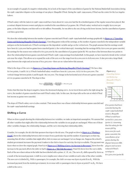
- Page 455: horizontal axis, measured between t
- Page 459 and 460: evenue curves unchanged. That is be
- Page 461 and 462: LEARNING OBJECTIVES 1. Understand n
- Page 463 and 464: Figure 21.14 Tangent Lines and the
- Page 465 and 466: TRY IT! Consider the following curv
- Page 467 and 468: the scaling of the vertical axis us
- Page 469 and 470: Figure 21.22 Intended Academic Majo
- Page 471 and 472: ANSWER TO TRY IT! Here are the time
- Page 473 and 474: What do you think is the argument m
- Page 475 and 476: Equation 22.14 The coefficient of r
- Page 477 and 478: Figure 22.2 A Decrease in Autonomou
- Page 479: NUMERICAL PROBLEMS 1. Suppose an ec


