A Digital Glacier Database for Svalbard - Norsk Polarinstitutt
A Digital Glacier Database for Svalbard - Norsk Polarinstitutt
A Digital Glacier Database for Svalbard - Norsk Polarinstitutt

You also want an ePaper? Increase the reach of your titles
YUMPU automatically turns print PDFs into web optimized ePapers that Google loves.
A <strong>Digital</strong> <strong>Glacier</strong> <strong>Database</strong> <strong>for</strong> <strong>Svalbard</strong><br />
Max König 1 , Christopher Nuth 2 , Jack Kohler 1 , Geir Moholdt 2 and Rickard Pettersen 3<br />
1 Norwegian Polar Institute, Fram Center, N-9296 Tromsø, Norway<br />
2 Dept. of Geosciences, University of Oslo, P.O.Box 1047 Blindern, 0316 Oslo Norway<br />
3 Dept. Of Earth Sciences, University of Uppsala, S-752 36 Uppsala<br />
Abstract<br />
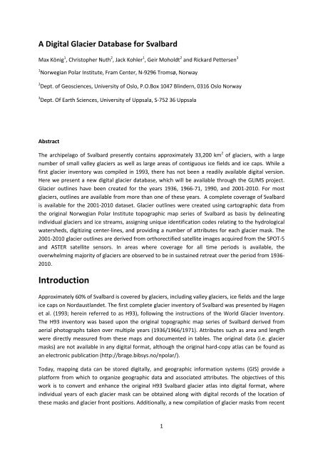
The archipelago of <strong>Svalbard</strong> presently contains approximately 33,200 km 2 of glaciers, with a large<br />
number of small valley glaciers as well as large areas of contiguous ice fields and ice caps. While a<br />
first glacier inventory was compiled in 1993, there has not been a readily available digital version.<br />
Here we present a new digital glacier database, which will be available through the GLIMS project.<br />
<strong>Glacier</strong> outlines have been created <strong>for</strong> the years 1936, 1966-71, 1990, and 2001-2010. For most<br />
glaciers, outlines are available from more than one of these years. A complete coverage of <strong>Svalbard</strong><br />
is available <strong>for</strong> the 2001-2010 dataset. <strong>Glacier</strong> outlines were created using cartographic data from<br />
the original Norwegian Polar Institute topographic map series of <strong>Svalbard</strong> as basis by delineating<br />
individual glaciers and ice streams, assigning unique identification codes relating to the hydrological<br />
watersheds, digitizing center-lines, and providing a number of attributes <strong>for</strong> each glacier mask. The<br />
2001-2010 glacier outlines are derived from orthorectified satellite images acquired from the SPOT-5<br />
and ASTER satellite sensors. In areas where coverage <strong>for</strong> all time periods is available, the<br />
overwhelming majority of glaciers are observed to be in sustained retreat over the period from 1936-<br />
2010.<br />
Introduction<br />
Approximately 60% of <strong>Svalbard</strong> is covered by glaciers, including valley glaciers, ice fields and the large<br />
ice caps on Nordaustlandet. The first complete glacier inventory of <strong>Svalbard</strong> was presented by Hagen<br />
et al. (1993; herein referred to as H93), following the instructions of the World <strong>Glacier</strong> Inventory.<br />
The H93 inventory was based upon the original topographic map series of <strong>Svalbard</strong> derived from<br />
aerial photographs taken over multiple years (1936/1966/1971). Attributes such as area and length<br />
were directly measured from these maps and documented in tables. The original data (i.e. glacier<br />
masks) are not available in any digital <strong>for</strong>mat, although the original hard-copy atlas can be found as<br />
an electronic publication (http://brage.bibsys.no/npolar/).<br />
Today, mapping data can be stored digitally, and geographic in<strong>for</strong>mation systems (GIS) provide a<br />
plat<strong>for</strong>m from which to organize geographic data and associated attributes. The objectives of this<br />
work is to convert and enhance the original H93 <strong>Svalbard</strong> glacier atlas into digital <strong>for</strong>mat, where<br />
individual years of each glacier mask can be obtained along with digital records of the location of<br />
these masks and glacier front positions. Additionally, a new compilation of glacier masks from recent<br />
1
satellite images is created, to provide the most up-to-date glacier inventory of the <strong>Svalbard</strong><br />
archipelago.<br />
Regional Context<br />
<strong>Svalbard</strong> is a high arctic archipelago located north of mainland Norway between Greenland and<br />
Novaya Zemlya at approximately 78° N 16° E (Figure 1). <strong>Svalbard</strong>’s location between the Fram Strait<br />
and the Barents Sea at the outer reaches of the North Atlantic warm water current (Loeng, 1991)<br />
results in <strong>Svalbard</strong> experiencing a relatively warm and variable climate as compared to other regions<br />
at the same latitude. The winter sea ice cover of the Arctic Ocean to the North limits moisture supply<br />
while in the region South of <strong>Svalbard</strong> cyclones gain strength as storms move northward (Tsukernik et<br />
al., 2007). These geographical and meteorological conditions make the climate of <strong>Svalbard</strong> not only<br />
extremely variable (spatially and temporally), but also sensitive to deviations in both the heat<br />
transport from the south and the sea ice conditions to the north (Isaksson et al., 2005).<br />
The <strong>Svalbard</strong> archipelago comprises four major islands with a total area of ~61,000 km 2 , of which<br />
roughly 60% is covered by glaciers (Hagen et al., 1993). <strong>Glacier</strong> types include valley glaciers, ice fields<br />
and ice caps. <strong>Svalbard</strong> glaciers are generally polythermal (Björnsson et al., 1996; Hamran et al., 1996;<br />
Jania et al., 2005; Palli et al., 2003), and many of them are surge type (Hamilton and Dowdeswell,<br />
1996; Jiskoot et al., 2000; Murray et al., 2003b; Sund et al., 2009). Of the ~1,100 glaciers on <strong>Svalbard</strong><br />
that are larger than 1 km 2 , less than 20% of these terminate in tidewater, while the remainder<br />
terminate on land. Typical <strong>Svalbard</strong> glaciers are characterized by low velocities (
the last two digits indicate the specific glacier. In many cases, these codes referred to more than one<br />
glacier, which can be potentially divided into two or more glaciers based upon the locations of medial<br />
moraines. In addition, many glaciers containing single identification codes have divided into two or<br />
more individual glacier units through the ongoing frontal retreat in <strong>Svalbard</strong>. To account <strong>for</strong> this, we<br />
introduce a decimal into the original glacier codes. This maintains the original system while allowing<br />
<strong>for</strong> future progression and changes of the glaciers. The decimal also allows us to account <strong>for</strong> glaciers<br />
and snow patches smaller than 1 km 2 , which will receive the same identification code that ends with<br />
“99” but with an increasing decimal <strong>for</strong> each individual small glacier or snow patch (i.e. XXX99.01,<br />
XXX99.02).<br />
Since the original glacier atlas data are not digital, and due to the multiple year compilation of that<br />
database, this task requires re-compiling all glacier masks. All map data from the Norwegian Polar<br />
Institute was digitalized in the 1990s, which <strong>for</strong>ms the basis <strong>for</strong> this glacier inventory re-compilation.<br />
Many glaciers in <strong>Svalbard</strong> are valley-type, which are easily divisible into glacier masks. However, most<br />
of the glacier area comprises connected ice fields that drain into separate valleys. To divide these<br />
into individual glacier units we follow the principle of hydrological drainage divides based upon<br />
surface topography. We use a compilation of older and newer contour lines and <strong>Digital</strong> Elevation<br />
Models as well as satellite images to help interpret the border between individual glacier units. The<br />
hydrological approach based upon topography does not account <strong>for</strong> ice flow, e.g. ice may flow in a<br />
different direction than what the surface topography suggests and the ice divide may not always<br />
coincide with the topographic divide. While these masks and divides are derived with the best<br />
possible data at the present time, we acknowledge that errors and mistakes may occur, and<br />
there<strong>for</strong>e hope to create a transparent database where mistakes, if found, can be adjusted and<br />
corrected as further in<strong>for</strong>mation is acquired.<br />
It is important to note that the glacier inventory presented in this paper follows the original H93<br />
glacier atlas, using the same definition of individual glaciers, drainage basins and identification codes.<br />
The Global Land Ice Measurements from Space (GLIMS) project follows a somewhat different<br />
definition of glaciers and identification codes (Raup and Khalsa, 2010). Within GLIMS, <strong>for</strong> example,<br />
glaciers sharing one and the same terminus are defined as one glacier unit, whereas in H93 individual<br />
ice streams may be defined as separate glaciers even though sharing the same terminus. The glacier<br />
inventory presented in this paper will eventually be available in two versions, one available through<br />
the Norwegian Polar Institute following the H93 glacier definition and another one available through<br />
the GLIMS website following the GLIMS specifications as described in Raup and Khalsa (2010).<br />
Data<br />
The original Topographic Map Series of <strong>Svalbard</strong> (S100) – 1936 / 1966 / 1971<br />
The Norwegian Polar Institute (NPI) has created photogrammetric topographic maps <strong>for</strong> <strong>Svalbard</strong><br />
since the 1930s (Luncke, 1949). The original S100 Topographic Map Series of <strong>Svalbard</strong> is based on<br />
aerial photography and surveys taken during campaigns in 1936, 1938, 1960, 1966, and 1969-71. The<br />
first campaigns in 1936 and 1938 acquired oblique aerial photography from 2500-3000 m a.s.l. while<br />
the later campaigns acquired vertical aerial photography. The map series was created at 1: 100 000<br />
3
scale and with 50 meter contour interval. The accuracy and precision of the 1936/38 maps is limited<br />
due to the technology available at the time and to the relatively high flight altitudes. The uncertainty<br />
of glacier contours varies by elevation, with upper elevation contours less accurate than those at<br />
lower elevations due to the lower image contrast in the accumulation areas. In addition, the flight<br />
plan <strong>for</strong> the early aerial photography campaigns was preferentially flown around the coast looking<br />
inland, such that the distance to the image point of the higher-elevation areas was typically greater<br />
than that <strong>for</strong> lower elevation points (Nuth et al., 2007). The horizontal accuracy of the 1936/38 data<br />
can be 20-50 m, or even worse in some places. Topographic maps from 1960-1971 were created<br />
from vertical aerial photography obtained in late summer, which were analyzed using analog<br />
stereographic equipment to yield maps at a scale of 1 : 30 000 to 1 : 50 000. The horizontal<br />
uncertainty <strong>for</strong> the 1960-71 data is estimated to be 20-30 m (Harald Faste Aas, personal<br />
communication). The vertical uncertainty of the contours is found to be around 15-20 m compared to<br />
ICESat (Nuth et. al., 2010).<br />
The S100 topographic map series of <strong>Svalbard</strong> is thus a compilation of data from multiple years. The<br />
1936 dataset covers about 25% of the archipelago, mainly southern and western Spitsbergen. The<br />
1960-1971 data covers northern Spitsbergen and the eastern islands of Barentsøya and Edgeøya,<br />
about 50% of the entire archipelago. Data on Nordaustlandet were not collected until 1983 when a<br />
collaboration between The Scott Polar Research Institute (SPRI) and NPI acquired surface and bed<br />
elevations of the ice cap through radar echo sounding and pressure based altimetry (Dowdeswell et<br />
al., 1986). All archived map data were digitized in the 1990s, such that elevation contours, glacier<br />
outlines and coast lines became digitally available as shape files. The glacier outlines were, however,<br />
not divided into individual glaciers, but they only delineated connecting ice masses. There<strong>for</strong>e<br />
considerable analysis is required to convert the original, cartographic shapefile into a useable glacier<br />
database.<br />
The 1990 photogrammetric survey<br />
The 1990 campaign acquired vertical aerial images in late summer from a height of ca. 8000 m-a.s.l.<br />
The entire archipelago was covered, except <strong>for</strong> two swaths along the central ridge of the south<br />
eastern coast. The 1990 maps represent an improvement over the previous S100 maps in that the<br />
newer maps were made using digital photogrammetric techniques; automated image matching<br />
replaced the analogue stereoscopic plotter, and map quality became less dependent on the skill of<br />
the photogrammetrist.<br />
DEMs and orthophotos have been created from the 1990 images <strong>for</strong> approximately 30% of the<br />
archipelago after the photogrammetric survey. The basic NPI S100 database has been updated with<br />
these 1990 map products. However, the completion of the 1990 map products has officially been<br />
abandoned <strong>for</strong> a new generation of DEMs acquired from an ongoing aerial photogrammetric<br />
campaign started in 2007. The 1990 DEMs typically have a ground resolution of 20 m and a<br />
horizontal and vertical uncertainty of less than ±5 m (Nuth et al., 2007; Nuth et al., 2010).<br />
The Satellite dataset<br />
The main basis <strong>for</strong> the satellite-based glacier database is the IPY SPIRIT (SPOT 5 stereoscopic survey<br />
of Polar Ice: Reference Images and Topographies) project (Korona et al., 2009) which provided high<br />
resolution DEMs (40m/pixel) and orthophotos (5m/pixel) covering approximately 70% of the<br />
4
archipelago (Figure 2). The High Resolution Stereoscopic (HRS) Sensor onboard SPOT 5 contains 2<br />
telescopes looking <strong>for</strong>ward and backward 20° from nadir. The DEMs are automatically generated and<br />
geolocated with horizontal precisions better than 30 m (Bouillon et al., 2006; Nuth and Kääb, 2011,<br />
Nuth et al., in press). Vertical uncertainty is within ±10 m (Korona et al., 2009), although in practice it<br />
is often better than 5-8 m in <strong>Svalbard</strong> under optimal light conditions (high zenith angle) during<br />
acquisitions, <strong>for</strong> increasing contrast on the white glacier surfaces). To generate a complete satellite<br />
inventory, the missing areas from the IPY SPIRIT Project are covered using automatically generated<br />
ASTER DEMs and orthophotos from 2000-present (AST14DMO product from LPDAAC). The ASTER<br />
nadir- and back-looking cameras provide a base-to-height ratio of 0.6, and automatically generated<br />
DEMs have a horizontal uncertainty sometimes up to 3 pixels (90 m) and a vertical uncertainty of 15-<br />
20 m (Nuth and Kääb, 2011). All satellite datasets are first co-registered to the higher accuracy<br />
aerophotogrammetric products following Nuth and Kääb (2011), in which the horizontal correction<br />
parameters derived <strong>for</strong> the DEMs are applied directly to the orthophotos. The resulting horizontal<br />
geo-location is then as precise as ±10 m.<br />
Methodology<br />
Creating glacier outlines from cartographic data <strong>for</strong> the 1936/66/71 data set<br />
To initiate the transfer of individual glacier identification codes from H93 to digital media, we begin<br />
with the earliest cartographic shapefiles from the S100 map series (Figure 2a). Each individual glacier<br />
was separated from the original conglomerate polygon, and new metadata such as glacier name and<br />
ID added as an attribute. For individual valley glaciers not connected to a larger ice mass, the original<br />
polygon often needed minor adjustments, mainly accomplished by removing snow fields connected<br />
to the glacier surface that were originally included in the shapefile by the non-glaciologist<br />
cartographer. This was accomplished through visual inspection of orthorectified SPOT, ASTER and<br />
georectified Landsat images, and also using hillshades of the DEMs, where the mountain sides can be<br />
easily visualized.<br />
The larger interconnected ice masses also needed to be sub-divided into individual glaciers and ice<br />
streams. We follow the drainage basin divides as in H93, making only slight adjustments where our<br />
objective interpretations differ. Ice divides are manually digitized mainly using contours lines from<br />
the more recent DEMs (1990-present). As stated above, this hydrological approach <strong>for</strong> drainage basin<br />
division assumes ice flow in the direction of the surface slope. If actual ice flow diverges significantly<br />
from the apparent surface slope in the area of the basin drainage divides, this might lead to errors. In<br />
addition, determining individual glacier basins in the oldest dataset using more recent data can<br />
introduce errors. Nonetheless, the greatest apparent changes in <strong>Svalbard</strong> glaciers are occurring at<br />
the fronts, rather than at basin divides. A subset of the glacier database <strong>for</strong> the Kongsfjorden area<br />
can be seen in Figure 3, showing among others the 1936 outlines.<br />
Creating Outlines from cartographic data <strong>for</strong> the 1990 data set<br />
Most of the 1990 data cover glaciers where outlines <strong>for</strong> 1936-1971 are available as well (Figure 2b).<br />
Polygons of individual valley glaciers required little adjustment from the original 1990 cartographic<br />
data and were again taken entirely from the original data except <strong>for</strong> the removal of adjacent snow<br />
fields where necessary. For the larger interconnected ice masses, ice divides were not re-analyzed<br />
5
ut rather copied from the previous (1936/66/71) glacier outlines. The glacier identification codes<br />
were simply transferred from the older (S100) dataset to the 1990 dataset, where applicable. This<br />
method assumes that the accumulation area divides between ice masses have not changed<br />
significantly over the years. Again, most area changes of individual glaciers and ice streams occurs at<br />
the tongue of the glacier. Figure 3 shows frontal changes and outlines <strong>for</strong> 1990 in the Kongsfjorden<br />
area.<br />
Creating Outlines from satellite data <strong>for</strong> the 2001-2010 data set<br />
The satellite-derived glacier inventory dataset represents at present the only complete areal<br />
coverage of <strong>Svalbard</strong> derived within a short time span (Figure 2c). For this dataset, we update front<br />
positions (retreat or advance) by clipping or extending glacier outlines from the most recent mask<br />
(depending on availability in either the S100 or 1990 inventory). For glaciers experiencing large<br />
retreat, which is the case <strong>for</strong> most glaciers on <strong>Svalbard</strong>, the valley sides were also updated because<br />
there has also been concurrent areal shrinkage. The result <strong>for</strong> this in the Kongsfjorden area is again<br />
seen in Figure 3. In addition, some glaciers tagged with a single identification code in H93 have<br />
retreated into two or more separate glacier units. For these cases, the original 5 digit glacier<br />
identification codes are retained, but updated with a decimal digit to identify the new individual<br />
units. This will have an effect on the quantification of the number of glaciers in <strong>Svalbard</strong>.<br />
<strong>Glacier</strong> and snow patches smaller than 1 km 2<br />
The original inventory H93 did not specifically include glaciers smaller than 1 km 2 , although it did<br />
attempt to estimate the number and combined area of such units. Our new digital glacier inventory<br />
attempts to include all individual glaciers smaller than 1 km 2 . However, at present they do not have<br />
an individual 5 digit identification code, but rather a single unique identification code based upon the<br />
regional drainage basin (typically XXX99) followed by a unique decimal identifier. This was done both<br />
to maintain the original structure of the glacier inventory, as well as to include an estimate on the<br />
number and size of ice/snow patches less than 1km 2 . Uncertainty prevails in the determination of<br />
whether small features are indeed glaciers or rather a non-dynamic snow field; this decision is<br />
subjective and difficult to automate. Each unit in the glacier database is manually classified on a caseby-case<br />
basis using the plethora of satellite images (SPOT, ASTER and Landsat) as well as the original<br />
photographs from the aerial surveys to determine whether small snow fields indeed are a glacier.<br />
Results<br />
Early versions of the <strong>Svalbard</strong> glacier inventory have been used to study changes in glacier geometry<br />
and glacier elevation (Nuth et al., 2007). While a more complete analysis awaits completion of the<br />
final glacier inventory, the following is a preliminary analysis showing the potential of the new data<br />
set.<br />
Currently, there are over 1,100 glaciers in <strong>Svalbard</strong> larger than 1 km 2 , with the majority in the size<br />
class 10-30 km 2 (Figure 4). <strong>Glacier</strong>s or snow patches smaller than 1 km 2 comprise less than 1% of the<br />
total glaciated area. In combination with a digital elevation model (DEM), the glacier outlines can be<br />
used to determine glacier hypsometry, i.e. the glacier area size as a function of elevation. <strong>Glacier</strong><br />
6
hypsometry varies considerably around the archipelago (Figure 5), and depends on the underlying<br />
terrain. Region 3 and especially Region 4 are areas of higher topography, where glaciers reach<br />
elevations above 1000 m.a.s.l.<br />
The database and hypsometries can be used to make a rough estimate of equilibrium line altitudes<br />
<strong>for</strong> all of <strong>Svalbard</strong>. The accumulation-area ratio (AAR) is an easily-measured parameter strongly<br />
related to the long-term mass balance. Typical AAR values <strong>for</strong> glaciers in balance range from 0.4 – 0.8<br />
(Bahr et al., 2009). Using the glacier hypsometry and assuming a uni<strong>for</strong>m accumulation area ratio<br />
(AAR) of 0.6 (e.g. Moholdt et al., 2010), the equilibrium line altitude (ELA) can thus be found by<br />
choosing the elevation band delineating the upper 60% of the total area, the accumulation area.<br />
Figure 6 shows that ELAs calculated in this way are located at higher altitudes in the northern and<br />
central part of Spitsbergen, consistent with the lower precipitation amounts in that area (Hagen et<br />
al., 1993).<br />
Of course, <strong>Svalbard</strong> glaciers are not in balance, and AARs do vary even <strong>for</strong> glaciers in balance (Bahr et<br />
al., 2009), so that assuming a uni<strong>for</strong>m value of AAR = 0.6 is likely inappropriate <strong>for</strong> some glaciers or<br />
areas. Indeed, long-term mass balance measurements made on four glaciers in the area of Ny-<br />
Ålesund (Kohler, unpublished) show AAR ranging from 0.2 to 0.4. However, these glaciers in western<br />
<strong>Svalbard</strong> are in an area with significantly negative mass balance (Nuth et al., 2010). Applying a<br />
“standard” choice of AAR = 0.6 is appropriate <strong>for</strong> the entire archipelago, as a rough approximation;<br />
while ELA values so determined will vary with the AAR value used, the relative spatial distribution of<br />
ELAs is insensitive to AAR choice. With the caveats raised here, the geographic pattern of widely<br />
variable ELAs shown in Figure 6 is consistent with climatic differences across the island described in<br />
the Regional Context section.<br />
In southern Spitsbergen, we have nearly complete mapping coverage <strong>for</strong> 1936, 1990, and 2008<br />
(Figure 2), allowing us to calculate area change <strong>for</strong> the two periods 1936‐1990 and 1990‐2008. Figure<br />
7 shows the area change expressed in percent change per year. The largest area changes occur <strong>for</strong><br />
smaller glaciers in the first period. In the second period, there is an increase in the area lost <strong>for</strong> the<br />
low-altitude glaciers to the south. An increase in the rate of mass loss in western <strong>Svalbard</strong> has<br />
previously been inferred from DEMs and other elevation data (Kohler et al., 2007) and has been<br />
attributed to the concurrent long-term increase in summer temperature (Nordlie and Kohler, 2004)<br />
observed since the 1930s. Some glaciers in Figure 7 are seen to have had an increase in glacier area<br />
(blue colors); these glaciers underwent a surge between the times of two map pairs.<br />
Most glaciers—whether tidewater or land-terminating, large or small, debris-covered or<br />
comparatively clean ice types—have undergone retreat over both time periods detailed in Figure 7.<br />
This widespread and dominant retreat, occurring <strong>for</strong> such a wide range of glacier types and sizes, is in<br />
accordance with the observed climate change (Nordlie and Kohler, 2004). For the region shown in<br />
Figure 7, the total area retreat during the first period, last period, and the sum of both periods is,<br />
respectively, 832.5, 243.1, and 1075.6 km 2 , which compares to 4,961.6 km 2 total glacier area, as of<br />
2008.<br />
Conclusions and Future Perspectives<br />
The new digital inventory of <strong>Svalbard</strong> glaciers presented above contains data from multiple years,<br />
including 1936, 1938, 1960, 1966, 1969-71, 1990 and 2001-2010. The inventory derived from the<br />
7
latter, 21 st century satellite dataset is at present the only period <strong>for</strong> which there is a spatially<br />
complete glacier inventory of <strong>Svalbard</strong>. The inventory comprises glacier outlines in the <strong>for</strong>m of<br />
shapefiles and an associated attribute table describing each individual glacier. We envision a “living<br />
inventory” (dynamic inventory), which can be updated and expanded with additional glaciological<br />
data. A more complete database <strong>for</strong> example, will include glacier centerlines and lengths, glacier<br />
hypsometries, ELA and firn line estimates, thickness measurements and volume estimates as these<br />
become available. Official publication of the dataset will occur first through a digital portal operated<br />
by the Norwegian Polar Institute, and will also be sent into the GLIMS archives at the National Snow<br />
and Ice data Center (NSIDC). In addition, the dataset will be available through the CryoClim data<br />
portal. We envision a working database where publications on <strong>Svalbard</strong> glaciers can also be linked to<br />
the database through the unique glacier identification codes and there<strong>for</strong>e the database can function<br />
as a simple reference index <strong>for</strong> <strong>Svalbard</strong> glaciers.<br />
Acknowledgements<br />
We would like to thank Harald Faste Aas, Roger Willy Olaussen and Anders Skoglund <strong>for</strong> providing<br />
the topographic data and <strong>for</strong> advice regarding this data. Also, Boele Kuipers <strong>for</strong> advice on GIS<br />
matters. The ASTER orthorectified images and SilcAst DEMs were provided within the framework of<br />
the Global Land Ice Measurements from Space project (GLIMS) through the USGS LPDAAC and is<br />
courtesy of NASA/GSFC/METI/ERSDAC/JAROS and the US/Japan ASTER science team. The SPOT5-HRS<br />
orthorectified images and DEM were obtained through the IPY-SPIRIT project (Korona et al., 2009)©<br />
CNES 2008 and SPOT Image 2008 all rights reserved. This work is a contribution to the ESA Climate<br />
Change Initiative Project "<strong>Glacier</strong>s CCI" (Essential Climate Variable CCI ECV glaciers and ice caps). This<br />
work is in part funded by the Norwegian Space Centre as part of ESA’s PRODEX program through the<br />
CryoClim project.<br />
8
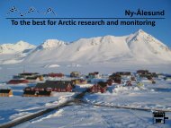
Figure 1: The <strong>Svalbard</strong> archipelago<br />
9
Figure 2a-c: <strong>Svalbard</strong> maps showing coverage of the three temporal datasets with glacier outlines<br />
derived from cartographic data (1936-1990) and SPOT images (2001-2010; ©CNES 2008)<br />
10
Figure 3: A subset of the database shows all available data at Brøggerhalvøya with a 2007 SPOT<br />
image (CNES 2008) as background. The colours of the glacier outlines correspond to the colours<br />
indicating data collection years in Figure 2. Retreat of the glaciers between 1936 and 2007 is clearly<br />
evident with a decrease of 3% glaciated area in Kongsfjorden. Centerlines <strong>for</strong> each glacier are also<br />
shown. We note that the glacier tongue to the far right is divided into individual tributaries following<br />
the glacier inventory by Hagen et al. (1993). GLIMS would consider these tributaries being part of a<br />
single glacier.<br />
11
Figure 4: Distribution of glaciers sizes <strong>for</strong> <strong>Svalbard</strong>. There are over 1,100 glaciers in <strong>Svalbard</strong> larger<br />
than 1 km 2 , with the majority in the size class 10-30 km 2 . <strong>Glacier</strong>s or snow patches smaller than 1 km 2<br />
comprise less than 1% of the total glaciated area.<br />
12
Figure 5: <strong>Glacier</strong> hypsometry <strong>for</strong> different regions on <strong>Svalbard</strong>.<br />
13
Figure 6: ELA distribution <strong>for</strong> <strong>Svalbard</strong>, estimated from individual glacier hypsometries and assuming<br />
constant AAR = 0.6. Estimated ELAs are located at higher altitudes in the northern and central part of<br />
Spitsbergen, corresponding to the lower precipitation amounts in that area (Hagen et al., 1993).<br />
14
Figure 7: Annual glacier area change in percentage per year <strong>for</strong> 1936 to 1990 and 1990 to 2008,<br />
relative to 1936 and 1990, respectively. <strong>Glacier</strong>s with an increase in glacier area (blue colors)<br />
underwent a surge between the two maps.<br />
15
References<br />
Bahr, D. B., M. Dyurgerov and M. F. Meier (2009). "Sea-level rise from glaciers and ice caps: A lower<br />
bound." Geophysical Research Letters 36.<br />
Björnsson, H., Y. Gjessing, S. E. Hamran, J. O. Hagen, O. Liestøl, F. Palsson, and B. Erlingsson (1996).<br />
The thermal regime of sub-polar glaciers mapped by multi-frequency radio-echo sounding,<br />
Journal of Glaciology, 42(140): 23– 32.<br />
Blaszczyk, M., J. A. Jania and J. O. Hagen. 2009. Tidewater glaciers of <strong>Svalbard</strong>: Recent changes and<br />
estimates of calving fluxes. Polish Polar Research, Vol. 30, no. 2, pp. 85–142.<br />
Bouillon, A., M. Bernard, P. Gigord, A. Orsoni, V. Rudowski and A. Baudoin (2006). "SPOT 5 HRS<br />
geometric per<strong>for</strong>mances: Using block adjustment as a key issue to improve quality of DEM<br />
generation." ISPRS Journal of Photogrammetry and Remote Sensing 60(3): 134 - 146.<br />
Dowdeswell, J., D. J. Dewry, A. P. R. Cooper, M. R. Gorman, O. Liestøl and O. Orheim (1986). "<strong>Digital</strong><br />
mapping of the Nordaustlandet ice caps from airborne geophysical investigation." Annals of<br />
Glaciology 8: 51-58.<br />
Hagen, J. O., J. Kohler, K. Melvold and J. G. Winther (2003a). "<strong>Glacier</strong>s in <strong>Svalbard</strong>: mass balance,<br />
runoff and freshwater flux." Polar Research 22(2): 145-159.<br />
Hagen, J. O., K. Melvold, F. Pinglot, and J. A. Dowdeswell (2003b). On the net mass balance of the<br />
glaciers and ice caps in <strong>Svalbard</strong>, Norwegian Arctic, Arctic Antarctic and Alpine Research,<br />
35(2): 264 – 270.<br />
Hagen, J. O., O. Liestøl, E. Roland and T. Jørgensen. (1993). <strong>Glacier</strong> atlas of <strong>Svalbard</strong> and Jan Mayen.<br />
Oslo.<br />
Hamilton, G., and J. Dowdeswell (1996). Controls on glacier surging in <strong>Svalbard</strong>, Journal of Glaciology,<br />
42(140): 157–168.<br />
Hamran, S. E., E. Aarholt, J. O. Hagen, and P. Mo (1996). Estimation of relative water content in a subpolar<br />
glacier using surface-penetration radar, Journal of Glaciology, 42(142): 533– 537.<br />
Hisdal, V. (1985). Geography of <strong>Svalbard</strong>, Norw. Polar Inst., Oslo.<br />
Humlum, O. (2002). Modelling late 20th-century precipitation in Nordenskiøld Land, <strong>Svalbard</strong>, by<br />
geomorphic means, Norwegian Journal of Geography, 56(2), 96–103.<br />
Isaksson, E., et al. (2005). Two ice-core delta O-18 records from <strong>Svalbard</strong> illustrating climate and seaice<br />
variability over the last 400 years, Holocene, 15(4): 501– 509.<br />
Jania, J., et al. (2005), Temporal changes in the radiophysical properties of a polythermal glacier in<br />
Spitsbergen, Annals of Glaciology, 42: 125 – 134.<br />
16
Jiskoot, H., T. Murray, and P. Boyle (2000). Controls on the distribution of surge-type glaciers in<br />
<strong>Svalbard</strong>,Journal of Glaciology, 46(154): 412 – 422.<br />
Kohler, J., T. D. James, T. Murray, C. Nuth, O. Brandt, N. E. Barrand, H. F. Aas and A. Luckman (2007).<br />
"Acceleration in thinning rate on western <strong>Svalbard</strong> glaciers." Geophysical Research Letters<br />
34(18): 5.<br />
Korona, J., E. Berthier, M. Bernard, F. Rèmy and E. Thouvenot (2009). "SPIRIT. SPOT 5 stereoscopic<br />
survey of Polar Ice: Reference Images and Topographies during the fourth International Polar<br />
Year (2007-2009)." ISPRS Journal of Photogrammetry and Remote Sensing 64(2): 204-212.<br />
Loeng, H. (1991). Features of the physical oceanographic conditions of the Barents Sea, Polar<br />
Research, 10(1): 5 – 18.<br />
Luncke, B. (1949). "Norges <strong>Svalbard</strong>- og ishavs- undersøkelsers kartarbeider og anvendelsen av skråfotogrammer<br />
tatt fra fly." <strong>Norsk</strong> <strong>Polarinstitutt</strong> Meddelelser 68.<br />
Moholdt, G., J. O. Hagen, T. Eiken and T. V. Schuler (2010). "Geometric changes and mass balance of<br />
the Austfonna ice cap, <strong>Svalbard</strong>." The Cryosphere 4: 1-14.<br />
Murray, T., T. Strozzi, A. Luckman, H. Jiskoot, and P. Christakos (2003). Is there a single surge<br />
mechanism? Contrasts in dynamics between glacier surges in <strong>Svalbard</strong> and other regions,<br />
Journal of Geophysical Research, 108(B5): 2237.<br />
Nordli, Ø. and J. Kohler. 2004: The early 20th century warming. Daily observations at Grønfjorden<br />
and Longyearbyen on Spitsbergen (2nd edition). DNMI/klima report, No. 12/03.<br />
Nuth, C., J. Kohler, H. F. Aas, O. Brandt and J. O. Hagen (2007). "<strong>Glacier</strong> geometry and elevation<br />
changes on <strong>Svalbard</strong> (1936-90): a baseline dataset." Annals of Glaciology 46: 106-116.<br />
Nuth, C. and A. Kääb (2011). Co-registration and bias corrections of satellite elevation data sets <strong>for</strong><br />
quantifying glacier thickness change, The Cryosphere, 5, 271-290.<br />
Nuth, C., G. Moholdt, J. Kohler, J. O. Hagen and A. Kääb (2010). "<strong>Svalbard</strong> glacier elevation changes<br />
and contribution to sea level rise." Journal of Geophysical Research-Earth Surface 115.<br />
Nuth, C., T. V. Schuler, J. Kohler, B. Altena and J. O. Hagen " Estimating the long term calving flux of<br />
Kronebreen, <strong>Svalbard</strong>, from geodetic elevation changes and mass balance modelling."<br />
Journal of Glaciology in press.<br />
Palli, A., J. C. Moore, and C. Rolstad (2003). Firn-ice transition-zone features of four polythermal<br />
glaciers in <strong>Svalbard</strong> seen by groundpenetrating radar, Annals of Glaciology, 37: 298 – 304.<br />
Raup, B. and S. Khalsa (2010). GLIMS Analysis Tutorial,<br />
[http://www.glims.org/MapsAndDocs/assets/GLIMS_Analysis_Tutorial_a4.pdf]<br />
Sand, K., J. G. Winther, D. Marechal, O. Bruland, and K. Melvold (2003). Regional variations of snow<br />
accumulation on Spitsbergen, <strong>Svalbard</strong>, 1997– 99, Nordic Hydrology, 34(1– 2), 17–32.<br />
Sund, M., T. Eiken, J. O. Hagen, and A. Kääb (2009). <strong>Svalbard</strong> surge dynamics derived from geometric<br />
changes, Annals of Glaciology, 50, 50–60.<br />
17
Tsukernik, M., D. N. Kindig, and M. C. Serreze (2007). Characteristics of winter cyclone activity in the<br />
northern North Atlantic: Insights from observations and regional modeling, Journal of<br />
Geophysical Research, 112.<br />
Winther, J. G., O. Bruland, K. Sand, A. Killingtveit, and D. Marechal (1998). Snow accumulation<br />
distribution on Spitsbergen, <strong>Svalbard</strong>, in 1997, Polar Research, 17(2): 155 – 164.<br />
18