Exhaustive Search, Combinatorial Optimization and Enumeration ...

Exhaustive Search, Combinatorial
Optimization and Enumeration:
Exploring the Potential of Raw Computing
Power
Jürg Nievergelt
ETH, 8092 Zurich, Switzerland
jn@inf.ethz.ch
Abstract. For half a century since computers came into existence, the
goal of finding elegant and efficient algorithms to solve “simple” (welldefined
and well-structured) problems has dominated algorithm design.
Over the same time period, both processingand storage capacity of
computers have increased by roughly a factor of a million. The next
few decades may well give us a similar rate of growth in raw computing
power, due to various factors such as continuingminiaturization, parallel
and distributed computing. If a quantitative change of orders of magnitude
leads to qualitative advances, where will the latter take place Only
empirical research can answer this question.
Asymptotic complexity theory has emerged as a surprisingly effective
tool for predictingrun times of polynomial-time algorithms. For NPhard
problems, on the other hand, it yields overly pessimistic bounds.
It asserts the non-existence of algorithms that are efficient across an
entire problem class, but ignores the fact that many instances, perhaps
includingthose of interest, can be solved efficiently. For such cases we
need a complexity measure that applies to problem instances, rather than
to over-sized problem classes.
Combinatorial optimization and enumeration problems are modeled by
state spaces that usually lack any regular structure. Exhaustive search
is often the only way to handle such “combinatorial chaos”. Several general
purpose search algorithms are used under different circumstances.
We describe reverse search and illustrate this technique on a case study
of enumerative optimization: enumeratingthe k shortest Euclidean spanningtrees.
1 Catching Up with Technology
Computer science is technology-driven: it has been so for the past 50 years,
and will remain this way for the foreseeable future, for at least a decade. That is
about as far as specialists can extrapolate current semiconductor technology and
foresee that advances based on refined processes, without any need for fundamental
innovations, will keep improving the performance of computing devices.
Moreover, performance can be expected to advance at the rate of “Moore’s law”,
V. Hlaváč, K. G. Jeffery, and J. Wiedermann (Eds.): SOFSEM 2000, LNCS 1963, pp. 18–35, 2000.
c○ Springer-Verlag Berlin Heidelberg 2000

Potential of Raw Computer Power 19
the same rate observed over the past 3 decades, of doubling in any period of 1
to 2 years. An up-to-date summary of possibilities and limitations of technology
can be found in [12].
What does it mean for a discipline to be technology-driven Whatarethe
implications
Consider the converse: disciplines that are demand-driven rather than technology-driven.
In the 60s the US stated a public goal “to put a man on the moon
by the end of the decade”. This well-defined goal called for a technology that
did not as yet exist. With a great national effort and some luck, the technology
was developed just in time to meet the announced goal — a memorable technical
achievement. More often than not, when an ambitious goal calls for the invention
of new technology, the goal remains wishful thinking. In such situations, it is
prudent to announce fuzzy goals, where one can claim progress without being
able to measure it. The computing field has on occasion been tempted to use this
tactic, for example in predicting “machine intelligence”. Such an elastic concept
can be re-defined periodically to mirror the current state-of-the-art.
Apart from some exceptions, the dominant influence on computing has been
a technology push, rather than a demand pull. In other words, computer architects,
systems and application designers have always known that clock rates,
flop/s, data rates and memory sizes will go up at a predictable, breath-taking
speed. The question was less “what do we need to meet the demands of a new
application” as “what shall we do with the newly emerging resources”. Faced
with an embarassment of riches, it is understandable that the lion’s share of
development effort, both in industry and in academia, has gone into developing
bigger, more powerful, hopefully a little better versions of the same applications
that have been around for decades. What we experience as revolutionary
in the break-neck speed with which computing is affecting society is not technical
novelty, but rather, an unprecedented penetration of computing technology
in all aspects of the technical infrastructure on which our civilization has come
to rely. In recent years, computing technology’s outstanding achievement has
been the breadth of its impact rather than the originality and depth of its scientific/technical
innovations. The explosive spread of the Internet in recent years,
based on technology developed a quarter-century ago, is a prominent example.
This observation, that computing technology in recent years has been
“spreading inside known territory” rather than “growing into new areas”, does
not imply that computing has run out of important open problems or new ideas.
On the contrary, tantalizing open questions and new ideas call for investigation,
as the following two examples illustrate:
1. A challenging, fundamental open problem in our “information age”, is
a scientific definition of information. Shannon’s pioneering information theory
is of unquestioned importance, but it does not capture the notion of
“information” relevant in daily life (“what is your telephone number”) or
in business transactions (“what is today’s exchange rate”). The fact that we
process information at all times without having a scientific definition of what
we are processing is akin to the state of physics before Newton: humanity

20 JürgNievergelt
has always been processing energy, but a scientific notion of energy emerged
only three centuries ago. This discovery was a prerequisite of the industrial
age. Will we ever discover a scientific notion of “information” of equal rigor
and impact
2. Emerging new ideas touch the very core of what “computing” means. Half
a century of computing has been based on electronic devices to realize a von
Neumann architecture. But computation can be modeled by many other
physical phenomena. In particular, the recently emerged concepts of quantum
computing or DNA computing are completely different models of computation,
with strikingly different strengths and weaknesses.
The reason fundamentally new ideas are not receiving very much attention at
the moment is that there is so much to do, and so much to gain, by merely
riding the wave of technological progress, e. g. by bringing to market the next
upgrade of the same old operating system, which will surely be bigger, if not
better. Whereas business naturally looks for short-term business opportunities,
let this be a call to academia to focus on long-term issues, some of which will
surely revolutionize computing in decades to come.
2 “Ever-Growing” Computing Power:
What Is It Good for
Computer progress over the past several decades has measured several orders of
magnitude with respect to various physical parameters such as computing power,
memory size at all hierarchy levels from caches to disk, power consumption,
physical size and cost. Both computing power and memory size have easily grown
by a factor of a million. There are good reasons to expect both computing power
and memory size to grow by the same two factors of a million over the next couple
of decades. A factor of 1000 can be expected from the extrapolation of Moore’s
law for yet another dozen years. Another factor of 1000, in both computing
power and memory size, can be expected from increased use of parallel and
distributed systems — a resource whose potential will be fully exploited only
when microprocessor technology improvement slows down.
With hindsight we know what these two factors of a million have contributed
to the state of the art — the majority of today’s computer features and applications
would be impossible without them. The list includes:
– graphical user interfaces and multimedia in general,
– end-user application packages, such as spreadsheets,
– data bases for interactive, distributed information and transaction systems,
– embedded systems, for example in communications technology.
Back in the sixties it was predictable that computing power would grow, though
the rapidity and longevity of this growth was not foreseen. People speculated
what more powerful computers might achieve. But this discussion was generally
limited to applications that were already prominent, such as scientific computing.

Potential of Raw Computer Power 21
The new applications that emerged were generally not foreseen. Evidence for this
is provided by quotes from famous pioneers, such as DEC founder Ken Olsen’s
dictum “there is no reason why anyone would want a computer in his home” ([9]
is an amusing collection of predictions).
If past predictions fell short of reality, we cannot assume that our gaze into
the crystal ball will be any clearer today. We do not know what problems can
be attacked with computing power a million times greater than available today.
Thus, to promote progress over a time horizon of a decade or more, experimenting
is a more promising approach than planning.
3 Uneven Progress in Algorithmics
After this philosophical excursion into the world of computing, let us now consider
the small but important discipline of algorithmics, the craft of algorithm
design, analysis and implementation. In the early days of computing, algorithmics
was a relatively bigger part of computer science than it is now — all computer
users had to know and program algorithms to solve their problem. Until
the seventies, a sizable fraction of computer science research was dedicated to
expand and improve our knowledge of algorithms.
The computer user community at large may be unaware that the progress of
algorithmics can be considered spectacular. Whereas half a century ago an algorithm
was just a prescription to be followed, nowadays an algorithm is a mathematical
object whose properties are stated in terms of theorems and proofs.
A large number of well-understood algorithms have proven their effectiveness,
embedded in program libraries and application packages. They empower users
to work with techniques that they could not possibly program themselves. Who
could claim, for example, to know and be able to program all the algorithms in
a symbolic computation system, or in a computational geometry library
Asymptotic complexity analysis has turned out to be a surprisingly effective
technique to predict the performance of algorithms. When we classify an algorithm
as running in time O(log n) orO(n log n), generously ignoring constant
factors, how could we expect to convert this rough measure into seconds It’s
easy: you time the program for a few small data sets, and extrapolate to obtain
an accurate prediction of running times for much larger data sets, as the measurements
in Table 1 illustrate.
By and large, the above claim of spectacular success is limited to algorithms
that run in polynomial time, said to be in the class P . We have become so used
to asymptotic complexity analysis that we forget to marvel how such a simple
formula such as “log n” yields such accurate timing information. But we may
marvel again when we consider the class of algorithms called NP-hard, which
presumably require time exponential in the size n of the data set.
For these hard problems, occasionally called intractable, wehaveatheory
that is not nearly as practical as the theory for P , because it yields overly
pessimistic bounds. Our current theory of NP-hard problems is modeled on the
same approach that worked so successfully for problems in P : prove theorems

22 JürgNievergelt
Table 1. Running times of Binary Search
n log n t bin search t/ log n
1 0 0.60
2 1 0.81 0.81
4 2 0.91 0.45
8 3 1.08 0.36
16 4 1.26 0.32
32 5 1.46 0.29
64 6 1.66 0.27
128 7 1.88 0.27
256 8 2.08 0.26
512 9 2.30 0.26
1024 10 2.51 0.25
2048 11 2.71 0.25
4096 12 2.96 0.25
8192 13 3.23 0.25
16384 14 3.46 0.25
that hold for an entire class C(n) of problems, parametrized by the size n of the
data. What is surprising, with hindsight, is that this ambitious sledge-hammer
approach almost always works for problems in P ! We generally find a single
algorithm that works well for all problems in C, from small to large, whose
complexity is accurately described by a simple formula for all values of n of
practical interest.
If we aim at a result of equal generality for some NP-hard problem class C(n),
the outcome is disappointing from a practical point of view, for two reasons:
1. Since the class C(n) undoubtedly contains many hard problem instances,
a bound that covers all instances will necessarily be too high for the relatively
harmless instances. And even though the harmless instances might be
a minority within the class C(n), they may be more representative of the
actual problems a user may want to solve.
2. It is convenient, but not mandatory, to be able to use a single algorithm
for an entire class C(n). But when this approach fails in practice we have
another option which is more thought-intensive but hopefully less computeintensive:
to analyze the specific problem instance we want to solve, and to
tailor the algorithm to take advantage of the characteristics of this instance.
In summary, the standard complexity theory for NP-hard problems asserts the
non-existence of algorithms that are efficient across an entire problem class, but
ignores the possibility that many instances, perhaps including those of interest,
canbesolvedefficiently.
An interesting and valuable approach to bypass the problem above is to
design algorithms that efficiently compute approximate solutions to NP-hard
problems. The practical justification for this approach is that an exact or optimal

Potential of Raw Computer Power 23
solution is often not required, provided an error bound is known. The limitation
of approximation algorithms is due to the same cause as for exact algorithms
for NP-hard problems: that they aim to apply to an entire class C(n), and thus
cannot take advantage of the features of specific instances. As a consequence,
if we insist on a given error bound, say 20 %, the approximation problem often
remains NP-hard.
There is a different approach to NP-hard problems that still insists on finding
exact or optimal solutions. We do not tackle an entire problem class C(n);
instead, we attack a challenging problem instance, taking advantage of all the
specific features of this individual instance. If later we become interested in
another instance of the same class C, the approach that worked for the first
instance will have to be reappraised and perhaps modified. This approach
changes the rules of algorithm design and analysis drastically: we still have to
devise and implement clever algorithms, but complexity is not measured asymptotically
in terms of n: it is measured by actually counting operations, disk
accesses, and seconds.
4 Exhaustive Search and Enumeration: Concepts and
Terminology
One of the oldest approaches to problem solving with the help of computers is
brute-force enumeration and search: generate and inspect all data configurations
in a large state space that is guaranteed to contain the desired solutions, and you
are bound to succeed — if you can wait long enough. Although exhaustive search
is conceptually simple and often effective, such an approach to problem solving is
sometimes considered inelegant. This may be a legacy of the fact that computer
science concentrated for decades on fine-tuning highly efficient polynomial-time
algorithms. The latter solve problems that, by definition, are said to be in P .
The well known class of NP-hard problems is widely believed to be intractable,
and conventional wisdom holds that one should not search for exact solutions,
but rather for good approximations. But the identification of NP-hard problems
as intractable is being undermined by recent empirical investigation of extremely
compute-intensive problems. The venerable traveling salesman problem is just
one example of a probably worst-case hard problem class where many sizable
instances turn out to be surprisingly tractable.
The continuing increase in computing power and memory sizes has revived
interest in brute-force techniques for a good reason. The universe of problems
that can be solved by computation is messy, not orderly, and does not yield, by
and large, to the elegant, highly efficient type of algorithms that have received
the lion’s share of attention of the algorithms research community. The paradigm
shift that may be changing the focus of computational research is that combinatorial
chaos is just as interesting and rewarding as well-structured problems.
Many “real” problems exhibit no regular structures to be exploited, and that
leaves exhaustive enumeration as the only approach in sight. And even though we
look in vain for order of magnitude asymptotic improvements due to “optimal”

24 JürgNievergelt
algorithms, there are order of magnitude improvements waiting to be discovered
due to program optimization, and to the clever use of limited computational
resources. It is a game of algorithm design and analysis played according to
a new set of rules: forget asymptotics and see what can be done for some specific
problem instance, characterized by some large value of n. The main weapon in
attacking instances of NP-hard problems, with an invariably irregular structure,
is always search and enumeration.
The basic concepts of search algorithms are well known, but the terminology
used varies. The following recapitulation of important concepts serves to
introduce our terminology.
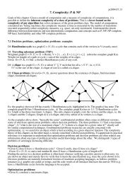
State space S. Discrete, often (but not necessarily) finite. Modeled as a graph,
S =(V,E) whereV is the set of vertices or nodes, E the set of edges (or
perhaps arcs, i. e. directed edges). Nodes represent states, arcs represent
relationships defined by given operators.
One or more operators, o: S → 2 S ,thepowersetofS. An operator transforms
a state s into a number of neighboring states that can easily be computed
given s. In the frequently occuring symmetric case, anoperatoro is its own
inverse in the following sense: s ′ ∈ o(s) implies s ∈ o(s ′ ).
Distinguished states, e. g. starting state(s), goal or target state(s). The latter
are usually defined by some target predicate t: S →{true, false}.
Objective function, cost function f : S → Reals. Serves to define an optimization
problem, where one asks for any or all states s that optimize (minimize
or maximize) f(s).
Search space. Often used as a synonym for state space. Occasionally it is useful
to make a distinction: a state space defines the problem to be solved, whereas
different search algorithms may traverse different subsets of S as their search
space.
Traversal. Sequentialization of the states of S. Common traversals are based
on imposing tree structures over S, called search tree(s) or search forest.
Search tree. A rooted, ordered tree superimposed on S. The children s 1 ...s f
of a node s are obtained by applying to s one of the operators defined on S,
and they are ordered (left-to-right order when drawn). The number f of
children of a node is called its fan-out. Nodes without children are called
leaves.
Search DAG. It is commonly the case that the same state s will be encountered
along many different paths from the root of a search tree towards its leaves.
Thus, the same state s may generate many distinct nodes of the same search
tree. By identifying (merging) all the tree nodes corresponding to the same
state s we obtain a directed acyclic graph, the search DAG.
DFS, BFS, etc. The most common traversal of S w. r. t. a given search tree
over S is depth-first search (DFS) or backtrack. DFS maintains at all times
a single path from the root to the current node, and extends this path whenever
possible. Breadth-first search (BFS) is also common, and can be likened
to wave-propagation outwards from a starting state. BFS maintains at all
times a frontier, or wave-front, that separates the states already visited from

Potential of Raw Computer Power 25
those yet to be encountered. Several other traversals are useful in specific
instances, such as best-first search, or iterative deepening.
Search structures. Every traversal requires data structures that record the
current state of the search, i. e. the subspace of S already visited. DFS
requires a stack, BFS a queue. The entire state S mayrequireamark(e.g.
a bit) for each state to distinguish states already visited from those not yet
encountered. The size of these data structures is often a limiting factor that
determineswhetherornotaspaceS can be enumerated with the memory
resources available.
Enumeration. A sequential listing of all the states of S, or of a subset S|t
consisting of all the target states s for which t(s) =true.
Output-sensitive enumeration algorithm. It is often difficult to estimate a priori
the size of the output of an enumeration. An appropriate measure of the
time required by an enumeration is therefore output-sensitive, whereby one
measures the time required to produce and output one state, the next in the
output sequence.
Search. The task of finding one, or some, but not necessarily all, states s that
satisfy some constraint, such as t(s) =true or f(s) isoptimal.
Exhaustive search. A search that is guaranteed to find all states s that satisfy
given constraints. An exhaustive search need not necessarily visit all of S in
every instance. It may omit a subspace S ′ of S on the basis of a mathematical
argument that guarantees that S ′ cannot contain any solution. In a worst
case configuration, however, exhaustive search is forced to visit all states
of S.
Examples of exhaustive search. Searching for a key x in a hash table is an
exhaustive search. Finding x, or determining that x is not in the table,
is normally achieved with just a few probes. In the worst case, however,
collisions may require probing the entire table to determine the status of
a key. By contrast, binary search is not exhaustive; when the table contains 3
or more keys, binary search will never probe all of them. Common exhaustive
search algorithms include backtrack, branch-and-bound, and sieves, such as
Erathostenes’ prime number sieve.
5 Reverse Search
The more information is known a priori about a graph, the less book-keeping
data needs to be kept during the traversal. Avis and Fukuda [2] presentaset
of conditions that enable graph traversal without auxiliary data structures such
as stacks, queues, or node marks. The amount of memory used for book-keeping
is constant, i. e. independent of the size of the graph. Their reverse search is
a depth-first search (DFS) that requires neither stack nor node markers to be
stored explicitly — all necessary information can be recomputed on the fly. Problems
to which reverse search applies allow the enumeration of finite sets much
larger than would be possible if a stack and/or markers had to be maintained.
Such enumeration is naturally time-consuming. But computing time is an elastic
resource — you can always wait “a little bit longer” — whereas memory is

26 JürgNievergelt
inelastic. When it is full, a stack or some other data structure will overflow and
stop the search. Thus, exhaustive search is often memory-bound rather than
time-bound.
Three conditions enable reverse search to enumerate a state space S =(V,E):
1. There is an adjacency operator or “oracle” A: S → 2 S ,thepowersetofS.
A assigns to any state s an ordered set A(s) =[s 1 ,...,s k ]ofitsneighbors.
Adjacency need not be symmetric, i. e. s ′ ∈ A(s) doesnotimplys ∈ A(s ′ ).
The pairs (s, s ′ )withs ′ ∈ A(s) define the set E of directed edges of S.
2. There is a gradient function g : S → S ∪{nil}, wherenil is a fictitious state
(a symbol) not in S. Astateswithg(s) =nil is called a sink of g. g assigns
to any state s a unique successor g(s) ∈ S ∪{nil} subject to the following
conditions:
– for any state s that is not a sink, i. e. g(s) ≠ nil, the pair (g(s),s) ∈ E,
i. e. s ∈ A(g(s)),
– g defines no cycles, i. e. g(g(...g(s) ...)) = s is impossible — hence the
name gradient.
Notice that when A is not symmetric, g-trajectories point in the opposite
direction of the arcs of E. Theno cycles condition in a finite space S implies
that g superimposes a forest, i. e. a set of disjoint trees, on S, wheretree
edges are a subset of E. Each sink is the root of such a tree.
3. It is possible to efficiently enumerate all the sinks of g before exploring all
of S.
The motivation behind these definitions and assumptions lies in the fact that A
and g together provide all the information necessary to manage a DFS that
starts at any sink of g. The DFS tree is defined by A and g as follows: The
children C(s) =[c 1 ,...,c f ] of any node s are those nodes s ′ culled from the set
A(s) =[s 1 ,...,s k ]forwhichg(s ′ )=s. Andtheorder[c 1 ,...,c f ] of the children
of s is inherited from the order defined on A(s).
A DFS usually relies on a stack for walking up and down a tree. An explicit
stack is no longer necessary when we can call on A and on g. Walking up the
DFS tree towards the root is accomplished simply by following the gradient
function g. Walking down from the root is more costly. Calling the adjacency
oracle from any node s yields a superset A(s) of the children of s. Eachs ′ in
A(s) must then be checked to see whether it is a child of s, as determined by
g(s ′ )=s.
Similarly, no data structure is required that marks nodes already visited. The
latter can always be deduced from the order defined on the set C(s) of children
and from two node identifiers: the current state and its immediate predecessor
in the DFS traversal.
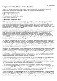
We explain how reverse search works on a simple example where every step
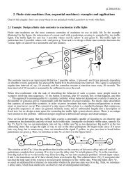
can be checked visually. Fig. 1 shows a hexagon (drawn as a circle) with vertices
labeled 1 ...6. Together with all 9 interior edges it makes up the complete
graph K 6 of 6 vertices shown at the top left. The other 14 copies of the hexagon,
each of them with 3 interior edges, show all the distinct triangulations of this

Potential of Raw Computer Power 27
labeled hexagon. The double-tipped arrows link each pair of states that are
neighbors under the only operator that we need to consider in this problem:
a diagonal flip transforms one triangulation into a neighboring one by exchanging
one edge for another. This, and the term diagonal, will be explained after we
introduce the notation for identifying edges and triangulations.
K 6
2
1
6
3
4
5
Fig. 1. The state space S of triangulations of a labeled hexagon

28 JürgNievergelt
The second ingredient required to implement reverse search is a suitable
gradient function g. We obtain this by imposing an arbitrary total order on
the state space S, accepting the fact that it breaks the elegant symmetry of
Fig. 1. Label an edge (i, j) with the ordered digit pair ij, i

Potential of Raw Computer Power 29
To understand the operator diagonal flip, observe that in every triangulation,
each interior edge is the diagonal of a quadrilateral, i. e. a cycle of length 4. In
triangulation #1 = 13.14.15, for example, 13 is the diagonal of the quadrilateral
with vertices 1, 2, 3, 4. By flipping diagonals in this quadrilateral, i. e. replacing
13 by its diagonal mate 24, we obtain triangulation #6 = 14.15.24. Thus, each of
the 14 triangulations has exactly 3 neighbors under the operator diagonal flip.
The 14 triangulations as vertices and the 14 ∗ 3/2 = 21 neighbor relations as
edges define the state space S =(V,E) of this enumeration problem.
Based on the total order shown in Fig. 2, define the gradient function g as
follows: g(s) is the “smallest” neighbor s ′ of s in lexicographic order, provided
s ′

30 JürgNievergelt
K6
#1 = 13.14.15
#2 = 13.14.46 #3 = 13.15.35
#6 = 14.15.24
#5 = 13.36.46
#4 = 13.35.36
#9 = 15.25.35
#8 = 15.24.25
#14 = 26.36.46
#11 = 24.26.46 #13 = 26.35.36 #12 = 25.26.35
#10 = 24.25.26
Fig. 3. Search tree defined by the gradient function g
with combinatorial assumptions, and vice versa. This interaction between geometric
and combinatorial constraints makes it difficult to predict, on an intuitive
basis, which problems are amenable to efficient algorithms, and which are not.
The difficulties mentioned are exacerbated when we aim at enumerating all
spatial configurations that meet certain specifications, not in any arbitrary order
convenient for enumeration, but rather in a prescribed order. Search techniques
impose their own restrictions on the order in which they traverse a search space,
and these may be incompatible with the desired order.
We present an example of a simple geometric-combinatorial search and enumeration
problem as an illustration of issues and techniques: the enumeration
of plane spanning trees over a given set of points in the plane, i. e. those trees
constructed with straight line segments in such a manner that no two edges

Potential of Raw Computer Power 31
intersect [8]. [2] present an algorithm for enumerating all plane spanning trees,
in some uncontrolled order that results from the arbitrary labeling of points.
We attack this same problem under the additional constraint that these plane
spanning trees are to be enumerated according to their total length (i. e. the sum
of the lengths of their edges), from short to long. We may stop the enumeration
after having listed the k shortest trees, or all trees shorter than a given bound c.
Fig. 4 lists the 10 shortest plane spanning trees among the 55 on the particular
configuration of 5 points with coordinates (0, 5), (1, 0), (4, 4), (5, 0), (7, 3).
14.89 15.41 15.85
15.87
15.89
15.99
16.29
16.38 16.38
16.41
Fig. 4. The 10 shortest plane spanning trees over five given points, in order of
increasing length
In trying to apply reverse search to a “k best problem” we face the difficulty
that the goal is not just to enumerate a set in some arbitrary, convenient order,
aswedidinSection5. In the case of enumerative optimization the goal is to
enumerate the elements of S from best to worst according to some objective
function f defined on S. One may wish to stop the enumeration after the k best
elements, or after having seen all elements s with f(s) ≤ c.
6.1 The Space of Plane Spanning Trees on a Euclidean Graph
Consider a graph G =(V,E,w) withn vertices p,q,r,... in V , weighted edges
e =(p, q) inE, and a weight function w : E → Reals. The set of spanning trees
over G has a well-known useful structure that is exploited by several algorithms,
in particular for constructing a minimum spanning tree (MST). The structure
isbasedonanexchangeoperator,anedge flip, and on a monotonicity property.
Let T be any spanning tree over G, e ′ an edge not in T , Ckt(e ′ ,T) the unique
path P in T that connects the two endpoints of e ′ ,ande any edge in P .The
edge flip T ′ = T − e + e ′ that deletes e from T and replaces it by e ′ creates
a new spanning tree T ′ that is adjacent to T .Ifw(e) >w(e ′ ) this edge flip
is profitable in the sense that |T ′ | < |T |, where|T | denotes the total length
of T . The remarkable fact exploited by algorithms for constructing a minimum
spanning tree (MST) is that in the space of all spanning trees over G, anylocal
minimum is also a global minimum. This implies that any greedy algorithm
based on profitable edge flips or on accumulating the cheapest edges (e. g. Prim,
Kruskal) converges towards an MST.

32 JürgNievergelt
In this paper we study Euclidean graphs and plane spanning trees. A Euclidean
graph is a complete graph whose vertices are points in the plane, and whose
edge weights are the distances between the endpoints of the edge. For p, q ∈ V
and e =(p, q), let |(p, q)| denote the length of edge e. For a Euclidean graph
it is natural to consider “plane” or non-crossing spanning trees, i. e. trees no
two of whose edges cross. It is well known and follows directly from the triangle
inequality that any MSTover a Euclidean graph is plane, i. e. has no crossing
edges.
In the following section, we define a search tree for enumerating all plane
spanning trees, in order of increasing total length, over a given point set in the
plane. This search tree is presented in such a form that standard tree traversal
techniques apply, in particular reverse search [2]. Specifically, we define a unique
root R which is an MST; and a monotonic gradient function g that assigns to
each tree T ≠ R atreeg(T )with|g(T )| ≤|T |. The gradient function g has the
property that, for any T ≠ R, some iterate g(...g(T )) equals R, i.e.R is a sink
of g; hence g generatesnocycles.Forefficiency’ssake,bothg and its inverse can
be computed efficiently.
For simplicity of expression we describe the geometric properties of the search
tree as if the configuration of points was non-degenerate in the sense that there
is a unique MST, and that any two distinct quantities (lengths, angles) ever
compared are unequal.
Unfortunately, the space of plane spanning trees over a Euclidean graph does
not exhibit as simple a structure as the space of all spanning trees. It is evident
that if T is a plane tree, an edge flip T ′ = T − e + e ′ may introduce cross-overs.
Thus, the geometric key issue to be solved is an efficient way of finding edge flips
that shorten the tree and avoid cross-over. We distinguish two cases:
6.1.1 Flipping edges in the Gabriel Graph. Consider any set C of noncrossing
edges over the given point set V , and any plane tree T contained in C.
Trivially, any edge flip limited to edges in C cannot introduce any cross-over. We
seek a set C, askeleton of G, that is dense enough so as to contain a sufficient
number of spanning trees, and has useful geometric properties. Among various
possibilities, the Gabriel Graph of V will do.
Definition 1. The Gabriel Graph GG(V )overapointsetV contains an edge
(p, q) iffnopointr in V −{p, q} is in the closed disk Disk(p, q) over the diameter
(p, q).
The useful geometric properties mentioned include:
1. GG(V ) has no crossing edges.
2. Consider any point x (not in V ) that lies inside Disk(p, q). Then |(x, p)| <
|(p, q)|, |(x, q)| < |(p, q)|, ∠(p, x, q) > 90 ◦ .
3. Any MSTover V is contained in GG(V ).
(Proof: consider any edge e of an MST. If there was any point p ∈ V inside
Disk(e), e could be exchanged for a shorter edge.)

Potential of Raw Computer Power 33
These geometric properties lead to a first rule.
Rule 1. Let T be a spanning tree over V that is not the (uniquely defined)
MST R. IfT is contained in GG(V ), let g(T )=T − e + e ′ ,wheree ′ is
the lexicographically first edge of R not in T ,ande is the longest edge in
Ckt(e ′ ,T).
Obviously, g(T )isclosertoR than T is, and if the MSTis unique, then |g(T )| <
|T |.
6.1.2 Flipping edges not in the Gabriel Graph. As a planar graph, the
Gabriel Graph GG(V ) has a sparse set of edges. Thus, the vast majority of
spanning trees over V are not contained in GG(V ), and hence Rule 1 applies
mostly towards the end of a g-trajectory, for spanning trees near the MST R.
For all other spanning trees, we need a rule to flip an edge (p, r) notinGG(V )in
such a way that the spanning tree gets shorter, and no cross-over is introduced.
Consider a tree T not contained in GG(V ), and hence is not an MST. Among
all point triples (p, q, r) such that (p, r) isinT , select the one whose ∠(p, q, r) is
maximum. The properties of the Gabriel Graph imply the following assertions:
∠(p, q, r) > 90 ◦ ,(p, r) isnotinGG(V ), |(p, q)| < |(p, r)| and |(q, r)| < |(p, r)|.
Rule 2. With the notation above, let g(T )=T − (p, r)+e ′ ,wheree ′ is either
(p, q) or(q, r), chosen such that g(T ) is a spanning tree.
As mentioned, |g(T )| < |T |. Fig.5 illustrates the argument that this edge flip
does not introduce any crossing edges. At left, consider the possibility of an
edge e one of whose endpoints u lies in the triangle (p, q, r). This contradicts the
assumption that ∠(p, q, r) is maximum. At right, consider the possibility of an
edge e =(u, v) that crosses both (p, q) and(q, r). Then ∠(u, q, v) > ∠(p, q, r),
again a contradiction. Thus, neither (p, q) nor(q, r) cause a cross-over if flipped
for (p, r).
These two rules achieve the goal of finding edge flips that
– shorten the tree, and
– avoid cross-over.
Thus, after a problem-specific detour into geometry, we are back at the point
where a general-purpose tool such as reverse search can take over.
q
e
q
p
u u v
e
r
p
r
Fig. 5. The assumption of new cross-overs contradicts the choice of “angle(p,q,r)
is maximum”

34 JürgNievergelt
7 The Craft of Attacking Hard Problem Instances
Exhaustive search is truly a creation of the computer era. Although the history of
mathematics records amazing feats of paper-and-pencil computation, as a human
activity, exhaustive search is boring, error-prone, exhausting, and never gets very
far anyway. As a cautionary note, if any is needed, Ludolph van Ceulen died of
exhaustion in 1610 after using regular polygons of 2 62 sides to obtain 35 decimal
digits of p — they are engraved on his tombstone.
With the advent of computers, experimental mathematics became practical:
the systematic search for specific instances of mathematical objects with desired
properties, perhaps to disprove a conjecture or to formulate new conjectures
based on empirical observation. Number theory provides a fertile ground for
the team computation + conjecture, and Derrick Lehmer was a pioneer in using
search algorithms such as sieves or backtrack in pursuit of theorems whose proof
requires a massive amount of computation [6]. We make no attempt to survey
the many results obtained thanks to computer-based mathematics, but merely
recall a few as entry points into the pertinent literature:
– the continuing race for large primes, for example Mersenne primes of
form 2 p − 1,
– the landmark proof of the “four-color theorem” by Appel and Haken [1],
– more recent work in Ramsey theory or cellular-automata [5].
For such cases we need a complexity measure that applies to problem instances,
rather than to over-sized problem classes. Counting individual operations and
measuring the running time of numerous procedures is a laborious exercise.
Again we marvel at the surprising practical effectiveness of the asymptotic complexity
analysis of algorithms — nothing of comparable elegance is in sight when
we attack hard problem instances.
The algorithm designer faces different challenges when attacking an instance
as compared to inventing an algorithm that solves a problem class. For the second
case we have many paradigms such as divide-and-conquer, greedy algorithms, or
randomization. The designer’s problem is to discover and prove mathematical
properties that greatly reduce the number of operations as compared to a bruteforce
approach. When attacking a problem instance we expect a priori that there
is nothing much cleverer than brute-force, and that we will use one of half a dozen
general purpose search algorithms. The main difficulty is algorithm and program
optimization.
Unfortunately, the discipline of algorithm and program optimization so far
has resisted most efforts at systematization. Several recent Ph. D. thesis’ have
attempted to extract general rules of how to attack compute-intensive problem
instances from massive case studies [4,3,7]. Data allocation on disk is a central
issue, trying to achieve some locality of data access despite the combinatorial
chaos typical of such problems. In problems involving retrograde analysis
(e. g. [11,13]), where every state (e. g. a board position in a game) in the state
space is assigned a unique index in a huge array, construction of a suitable index
function is critical. Since such computations may run for months and generate

Potential of Raw Computer Power 35
data bases of many GigaBytes, independent verification of the result is a necessity.
Some of the experience gained is summarized in [10].
Attacking computationally hard problem instances has so far never been
near the center of algorithm research. It has rather been relegated to the niche
of puzzles and games, pursued by a relatively small community of researchers.
The experience gained is more a collection of individual insights rather than
a structured domain of knowledge. As computing power keeps growing and people
attack harder problems, we will often encounter problems that must be tackled
as individual instances, because no algorithm that applies to a large class
will be feasible. Thus, it is a challenge to the computing research community to
turn individual insights into a body of knowledge, and to develop a complexity
theory of problem instances.
References
1. K. Appel and W. Haken. The Solution of the Four-Color-Map Problem. Scientific
American, pages 108–121, October 1977. 34
2. D. Avis and K. Fukuda. Reverse Search for Enumeration. Discrete Apllied Mathematics,
65:21–46, 1996. 25, 31, 32
3. A Bruengger. Solving hard combinatorial optimization problems in parallel. Two
case studies. PhD thesis, ETH Zurich, 1997. 34
4. R. Gasser. Harnessing computational resources for efficient exhaustive search. PhD
thesis, ETH Zurich, 1995. 34
5. J. Horgan. The Death of Proof. Scientific American, pages 74–82, 1993. 34
6. D. H. Lehmer. The machine tools of combinatorics. In E. F. Beckenbach, editor,
Applied combinatorial mathematics, chapter 1, pages 5–31. Wiley, NY, edition,
1964. 34
7. A Marzetta. ZRAM: A library of parallel search algorithms and its use in enumeration
and combinatorial optimization. PhD thesis, ETH Zurich, 1998. 34
8. A. Marzetta and J. Nievergelt. Enumerating the k best plane spanningtrees. In
Computational Geometry — Theory and Application, 2000. To appear. 31
9. H. Maurer. Forecasting: An impossible necessity. In Symposium Computer and
Information Technology, http://www.inf.ethz.ch/latsis2000/, Invited Talk. ETH
Zurich. 2000. 21
10. J. Nievergelt, R. Gasser, F. Mäser, and C. Wirth. All the needles in a haystack:
Can exhaustive search overcome combinatorial chaos In J. van Leeuwen, editor,
Computer Science Today, Lecture Notes in Computer Science LNCS 1000, pages
254–274. Springer, 1995. 35
11. K. Thomson. Retrograde analysis of certain endgames. ICCA J., 9(3):131–139,
1986. 34
12. H. van Houten. The physical basis of digital computing. In Symposium Computer
and Information Technology, http://www.inf.ethz.ch/latsis2000/, Invited
Talk. ETH Zurich. 2000. 19
13. C. Wirth and J. Nievergelt. Exhaustive and heuristic retrograde analysis of the
KPPKP endgame. ICCA J., 22(2):67–81, 1999 34