EMSO Manual - Ufrgs

EMSO
Manual
Rafael de Pelegrini Soares
www.rps.eng.br
LastChangedDate: 2007-08-30 11:22:15 -0300 (Qui, 30 Ago 2007)

Contents
I User’s Guide 1
1 Introduction 2
1.1 What is EMSO and EML . . . . . . . . . . . . . 3
1.2 Why use EMSO . . . . . . . . . . . . . . . . . . 3
1.2.1 Easy FlowSheet building . . . . . . . . . . 3
1.2.2 Integrated Graphical Interface . . . . . . . 3
1.2.3 Open-Source Model Library . . . . . . . . 3
1.2.4 Object-Oriented Modeling Language . . . 3
1.2.5 Multi-Platform system . . . . . . . . . . . 4
1.2.6 Fast and Transparent Setup . . . . . . . . 4
1.2.7 Solution Power . . . . . . . . . . . . . . . 4
1.2.8 Modeling of discontinuous process . . . . . 4
1.2.9 Operational procedures scripts . . . . . . . 5
1.2.10 Optimization . . . . . . . . . . . . . . . . 5
1.2.11 Parameter Estimation . . . . . . . . . . . 5
1.2.12 Open Interfaces . . . . . . . . . . . . . . 5
1.2.13 Open Engine API . . . . . . . . . . . . . 5
1.3 Installation . . . . . . . . . . . . . . . . . . . . . 6
1.3.1 Installing EMSO in win32 platforms . . . . 6
1.3.2 Installing EMSO in POSIX platforms . . . 6
2 Overview 8
2.1 EMSO Basics . . . . . . . . . . . . . . . . . . . 9
2.2 Running EMSO . . . . . . . . . . . . . . . . . . 9
2.2.1 Starting EMSO in win32 platforms . . . . 9
ii

2.2.2 Starting EMSO in POSIX platforms . . . . 9
2.3 EMSO graphical interface . . . . . . . . . . . . . 9
2.4 Tutorials . . . . . . . . . . . . . . . . . . . . . . 11
2.4.1 Three Tank FlowSheet . . . . . . . . . 12
3 EMSO Modeling Language 18
3.1 Modeling basics . . . . . . . . . . . . . . . . . . 19
3.1.1 Object Oriented Modeling . . . . . . . . . 19
3.1.2 Writing EMSO Entities . . . . . . . . . . 20
3.1.3 Documenting with Comments . . . . . . . 20
3.1.4 Types . . . . . . . . . . . . . . . . . . . . 21
3.1.5 Using files . . . . . . . . . . . . . . . . . 22
3.2 Model . . . . . . . . . . . . . . . . . . . . . . . 23
3.2.1 Parameters . . . . . . . . . . . . . . . . . 24
3.2.2 Variables . . . . . . . . . . . . . . . . . . 25
3.2.3 Composition in Models . . . . . . . . . . 26
3.2.4 Equations . . . . . . . . . . . . . . . . . 27
3.2.5 Initial Conditions . . . . . . . . . . . . . . 28
3.2.6 Abstract Models . . . . . . . . . . . . . 28
3.3 FlowSheet . . . . . . . . . . . . . . . . . . . . 28
3.3.1 Devices . . . . . . . . . . . . . . . . . 29
3.3.2 Connections . . . . . . . . . . . . . . . . 29
3.3.3 Specifications . . . . . . . . . . . . . . . 30
3.3.4 Options . . . . . . . . . . . . . . . . . . . 30
3.4 Optimization . . . . . . . . . . . . . . . . . . . . 30
3.4.1 Simple Optimizations . . . . . . . . . . . 32
3.4.2 Large-Scale Optimization . . . . . . . . . 33
3.4.3 Options . . . . . . . . . . . . . . . . . . . 33
3.4.4 Dynamic Optimization . . . . . . . . . . . 34
3.5 Built-in Functions . . . . . . . . . . . . . . . . . 35
3.6 Units Of Measurement (UOM) . . . . . . . . . . 36

3.6.1 Fundamental Units . . . . . . . . . . . . . 36
3.6.2 Derived Units . . . . . . . . . . . . . . . 36
3.7 Solver Options . . . . . . . . . . . . . . . . . . . 40
4 Advanced Modeling 44
4.1 Arrays . . . . . . . . . . . . . . . . . . . . . . . 45
4.1.1 Vectors . . . . . . . . . . . . . . . . . . . 45
4.1.2 Multidimensional Arrays . . . . . . . . . . 46
4.1.3 Equation Expansion . . . . . . . . . . . . 46
4.1.4 Array Functions . . . . . . . . . . . . . . 47
4.1.5 Loop For . . . . . . . . . . . . . . . . . . 48
4.2 Conditional Modeling . . . . . . . . . . . . . . . 48
5 Calculation Object Interface 49
5.1 Introduction . . . . . . . . . . . . . . . . . . . . 50
5.1.1 What is Plugin . . . . . . . . . . . . . 50
5.1.2 Why use a Plugin . . . . . . . . . . . 50
5.1.3 The Plugin Basics . . . . . . . . . . . . 50
5.2 Using Plugins . . . . . . . . . . . . . . . . . . 51
5.2.1 Using Plugins in Models . . . . . . . . 51
II Programming Guide 54
6 Developing new Plugin Services 55
6.1 Interface Specification . . . . . . . . . . . . . . . 56
6.1.1 Create Function . . . . . . . . . . . . . . 56
6.1.2 Destroy Function . . . . . . . . . . . . . . 58
6.1.3 Verification Functions . . . . . . . . . . . 58
6.1.4 Calculation Function . . . . . . . . . . . . 60
6.2 Writing new Plugin Services . . . . . . . . . . . 63
6.2.1 Writing Plugin Services in Fortran . . . 63
6.2.2 Writing Plugin Services in C . . . . . . 63

6.2.3 Writing Plugin Services in C++ . . . . 64
6.3 Documenting Plugin Services . . . . . . . . . . 64
7 Developing new Solvers 65
7.1 NLA Solvers . . . . . . . . . . . . . . . . . . . . 66
7.1.1 Residuals Function . . . . . . . . . . . . . 66
7.1.2 Jacobian . . . . . . . . . . . . . . . . . . 67
7.1.3 Matrix Multiplication . . . . . . . . . . . 68
7.1.4 Create and Destroy Functions . . . . . . . 69
7.1.5 Solve Function . . . . . . . . . . . . . . . 71
7.2 DAE Solvers . . . . . . . . . . . . . . . . . . . . 72
7.2.1 Create and Destroy Functions . . . . . . . 73
7.2.2 Step Function . . . . . . . . . . . . . . . 74
7.3 Writing new Solver Services . . . . . . . . . . . . 75
7.3.1 Writing External Solver Services in Fortran 75
7.3.2 Writing External Solver Services in C . . . 76
7.3.3 Writing External Solver Services in C++ . 76
7.4 Documenting Solver Services . . . . . . . . . . . 76

License
EMSO alpha version License
(C) 2004-2007 ALSOC.
(Based on code from Rafael de Pelegrini Soares - www.rps.eng.br, (C)
2002-2004)
All rights reserved.
THIS SOFTWARE IS AT ALPHA STAGE AND CAN BE USED FOR EVALUATION
PURPOSES ONLY. NO USE OR DISTRIBUTION OF THIS SOFTWARE IS
GRANTED WITHOUT WRITTEN AUTHORIZATION OF THE COPYRIGHT HOLDER.
Except where otherwise noted, all of the documentation and
software included in this package is copyrighted by Rafael de
Pelegrini Soares. After the installation check the "license"
directory in order to see all third part software used by EMSO
and their respective licenses.
THIS SOFTWARE IS PROVIDED "AS-IS", WITHOUT ANY EXPRESS OR
IMPLIED WARRANTY. IN NO EVENT SHALL THE AUTHOR BE HELD LIABLE
FOR ANY DAMAGES ARISING FROM THE USE OF THIS SOFTWARE.
Rafael de Pelegrini Soares - www.rps.eng.br
Chemical Engineering M.Sc. at GIMSCOP a UFRGS.
EMSO is a trademark of UFRGS (Universidade Federal do Rio
Grande do Sul) All other registered or pending trademarks
mentioned in this manual are considered the sole property of
their respective owners. All rights reserved.
a Group of Integration, Modeling, Simulation, Control, and Optimization of Processes - Chemical Engineering
Department - Federal University of Rio Grande do Sul (UFRGS)
vi

Acknowledgments
Thank to all the people who sent me corrections and improvement
suggestions to both the manual and software. In special I would
like to thank the main EMSO users Argimiro R. Secchi and Paula
B. Staudt for helping me to disclose many missing aspects.
I would like to thank the authors of the following softwares libraries
for permitting the use of their code in EMSO:
DASSLC :
FOX-Toolkit :
FXScintilla :
RCOMPLEX :
SUNDIALS :
UMFPACK :
a solver for differential-algebraic equation systems
www.enq.ufrgs.br/enqlib/numeric/;
a C++ based Toolkit for developing Graphical User Interfaces
easily and effectively
www.fox-toolkit.org;
an implementation of Scintilla 1 for the FOX-Toolkit
www.nongnu.org/fxscintilla;
a solver for constrained nonlinear optimization.
www.enq.ufrgs.br/enqlib/numeric/;
suite of codes consisting of the solvers CVODE, KINSOL,
and IDA, and variants of these
www.llnl.gov/CASC/sundials/;
a set of routines for solving unsymetric sparse linear systems
www.cise.ufl.edu/research/sparse/umfpack;
Ipopt :
a software package for large-scale nonlinear optimization.
https://projects.coin-or.org/Ipopt;
In the development process the author proposed several improvements
and bug-fixes sent to the original authors to be shared with
the community. The source code of all the above cited softwares
can be obtained in the respective URL. Any further explanation
about how such softwares are used in EMSO can be obtained with
the author - www.rps.eng.br.
1 Scintilla is a free source code editing component, see www.scintilla.
org.
vii

Symbols and Conventions
In this document the following notations are used:
Piece of code: piece of code written in the EMSO modeling
language or console outputs:
1 Model tank
2 # body of the model
3 end
Code Identifier: emphasize identifiers that are commands,
file names and related entities.
Note: a note, for instance: EMSO is an equation based description
system, therefore the order of the equations does not matter.
Warning: a warning advertise, for instance: a .mso file free of
syntax errors still can have consistency errors.
Tip: a tip for the user, for instance: always check EML for a
model before develop a new one.
Linux note: note specific for POSIX systems (Linux and Unix),
for instance: EMSO can be available for any POSIX compliant
system upon request.
Windows note: note specific for win32 systems (Windows 95
and above and Windows NT 4 and above), for instance: the
windows file system is not case sensitive.
Under construction: marks a section as not yet implemented
or documented.
viii

I. User’s Guide
1

1 Introduction
Go any further in reading this manual or using EMSO without read, understand and accept
the EMSO license, found on page vi.
In this chapter we will learn what is EMSO and why use it.
Contents
1.1 What is EMSO and EML . . . . . . . . . . . . . . . . . . . . . . 3
1.2 Why use EMSO . . . . . . . . . . . . . . . . . . . . . . . . . . . . 3
1.3 Installation . . . . . . . . . . . . . . . . . . . . . . . . . . . . . . . 6
2

1.1 What is EMSO and EML 3
1.1 What is EMSO and EML
EMSO stands for Environment for Modeling, Simulation and
Optimization. It is a complete graphical environment where the
user can model complex dynamic or steady-state processes by simply
selecting and connecting model blocks. In addition, the user
can develop new models using the EMSO modeling language or
using those already made from the EMSO Model Library (EML).
EML is an open source library of models written in the EMSO
modeling language. The EMSO modeling language is an objectoriented
language for modeling general dynamic or steady-state
processes.
1.2 Why use EMSO
1.2.1 Easy FlowSheet building
1.2.2 Integrated Graphical Interface
1.2.3 Open-Source Model Library
In this section we show the key concepts of EMSO and its advantages.
EMSO provides the facility of building complex process models,
called FlowSheets, by simply composing it with preexisting
blocks, called Models, and connecting them.
EMSO provides an integrated graphical interface where the user
can manage their .mso files. Multiple files can be opened simultaneously
and each file can contain an unlimited number of
Models, FlowSheets or Scripts. In the same interface the
user can run simulations and visualize the results besides a lot of
development facilities.
The .mso files coming with EMSO
are distributed under the terms of
the EMSO model license.
The EMSO distribution comes with a set of ready to use models
written in the EMSO modeling language – the EMSO Model Library
(EML). Therefore, complex FlowSheets can be built by
simply selecting EML models as Devices and connecting them.
EML is an open-source library and can be extended or modified
by the user.
1.2.4 Object-Oriented Modeling Language
EMSO provides a modeling language that allows the user to write
mathematical models almost as they would appear on paper. In

4 1 Introduction
addition, the language is fully object-oriented, allowing the user to
develop complex models by composing them with existent small
models or develop specific models by deriving standard ones.
All EML models are written in the EMSO modeling language and
are stored in plain text .mso files which can be edited or extended
by the user.
1.2.5 Multi-Platform system
EMSO is available for win32, POSIX (Linux and Unix) platforms.
Models developed in one platform can be freely interchanged between
others.
1.2.6 Fast and Transparent Setup
Process simulators in which models are not black-boxes pieces of
software obligatory have to translate the human readable description
to some solvable form. This translation step is called setup
phase.
In EMSO, the setup phase does not relies in the creation of intermediary
files, compilation, linkage or translation to another
language, the models are directly converted (in memory) to systems
of equations. This mechanism reduces the setup time by
orders of magnitude.
1.2.7 Solution Power
EMSO provides solvers for dynamic and steady-state systems
which are efficient in solving both small and large scale systems.
The solvers can make use of the dense or sparse linear algebra.
Actually there is no limit regarding problem size other than the
machine memory. In addition, new solvers can be interfaced to
EMSO and used in a seamless manner.
State of art techniques as automatic and symbolic differentiation
algorithms are built-in in EMSO. Furthermore, it has proved to
be one of the most time efficient tools when solving large scale
dynamic problems.
1.2.8 Modeling of discontinuous process
There are several processes which are in nature discontiuous, with
EMSO it is easy to model continuous-discrete (hybrid) systems
using conditional equations.

1.2 Why use EMSO 5
1.2.9 Operational procedures scripts
Under construction: To be implemented and documented.
1.2.10 Optimization
1.2.11 Parameter Estimation
Besides dynamic and steady simulation EMSO can be used to
find optimal solutions with respect to given criteria. The user
just need to formulate the optimization objective (lower cost,
maximum production, etc) and choose the optimization variables
(manipulated variables) in the Optimization environment and
let the system to find the best solution. See examples in the
ammonia opt.mso and flash opt.mso in the folder
/mso/sample/optimization.
EMSO can perform parameter estimation of dynamic and steadystate
models using the Estimation environment. See examples
in the BatchReactor.mso and sample est.mso files in
the /mso/sample/estim folder.
1.2.12 Open Interfaces
EMSO has a set of open interfaces that allow the user to load
at run-time third-party software encapsulated in dynamic link libraries.
(See Part II).
In addition, there are standard interfaces for implementing new
differential-algebraic equations (DAE), nonlinear algebraic equations
(NLA), and nonlinear optimization problem (NLP) solvers.
1.2.13 Open Engine API
AUTO2000 DAE can be
donwloaded at www.enq.ufrgs.
br/enqlib/numeric. See www.
peq.coppe.ufrj.br/auto_dae
for details.
EMSO is composed by two major softwares: the graphical interface
and the engine. The EMSO power in solving complex
large-scale dynamic problems is available to be embedded in third
party software through the EMSO engine open Application Program
Interface (API). Using this technology, EMSO installation
already provides an engine to build bifurcation diagrams using
AUTO2000 adapted to work with differential-algebraic equations
(DAE), and also SFunctions for simulating dynamic models
built with EMSO modeling language inside Matlab/Simulink R○
with continuous and discrete-time simulation. See the installation
procedure.

6 1 Introduction
1.3 Installation
EMSO is available for two main platform groups: win32 and
POSIX. Installation instructions for these platforms can be found
in subsection 1.3.1 and subsection 1.3.2 respectively.
1.3.1 Installing EMSO in win32 platforms
EMSO is compatible with a variety of win32 operational systems
(Windows 95, Windows NT 4, Windows XP and above).
In order to install EMSO in such systems one can just run the
installation package emso-win32-.exe available
at www.enq.ufrgs.br/alsoc and follow the on screen instructions.
MINGW may be download at
www.mingw.org and CYGWIN at
www.cygwin.com.
In order to use the EMSO-AUTO interface it is also necessary to
install the AUTO2000 DAE package, that can be downloaded at
www.enq.ufrgs.br/enqlib/numeric, using a Linux-like
environment for Windows, such as MINGW or CYGWIN in the location
/usr/local/auto/2000 dae. After the installation, just run
the script auto2000 dae provided in the root directory of the
AUTO2000 DAE, using the command source auto2000 dae.
There are some examples to test the installation in the directory
/usr/local/auto/2000 dae/demos/DAE. Copy the
file auto emso.exe from /bin in the same location
of the examples and execute the command @r-emso ab dae,
where ab dae is the name of the example to run, or put the
directory /bin in the PATH environment variable.
In order to use the EMSO-Matlab/Simulink interface, just copy
the files emso sf.dll and emsod sf.dll from the location
/interface/matlab to the working directory. In
the original location there are some MDL files to run some examples
in the Simulink.
1.3.2 Installing EMSO in POSIX platforms
POSIX is the name for a series of
standards being developed by the
IEEE that specify a Portable
Operating System interface. The
”IX” denotes the Unix heritage of
these standards.
EMSO is compatible with a variety of POSIX platforms (Linux,
Unix).
In order to install EMSO in such systems you have to download the
archive emso---.tar.gz
available at www.enq.ufrgs.br/alsoc.
For instance, emso-linux2-i386-0.9.53.tar.gz is the
installation archive for Linux version 2 or above platforms running
in an i386 compatible machine.

1.3 Installation 7
The installation procedure for the EMSO-AUTO interface is the
same as for win32 platform, described above, just skip the part
for the Linux-like environment for Windows.
In order to use the EMSO-Matlab/Simulink interface, just copy
the files emso sf.mexlx and emsod sf.mexlx from the location
/interface/matlab to the working directory.
In the original location there are some MDL files to run
some examples in the Simulink, if you can make Simulink work in
Linux.
Note: Installation packages for any POSIX compliant platform
can be produced upon request.
Once an archive compatible with your system was downloaded,
EMSO can be installed with the following commands:
$ tar -xzvf emso---.tar.gz
# sudo mv emso /usr/local
# sudo ln -sf /usr/local/emso/bin/emso /usr/bin/emso
Note: The EMSO executable is found at the bin directory, the
installation at /usr/local is not mandatory.

2 Overview
This chapter provides an overview about EMSO. First some basics are presented followed by
some tutorials. These tutorials teaches how to:
• build a FlowSheet composed by a set of predefine Models;
• check the consistency of a FlowSheet
• run a dynamic simulations and plot results;
• customize FlowSheet options.
Further, the EMSO modeling language for development of new models is introduced.
Contents
2.1 EMSO Basics . . . . . . . . . . . . . . . . . . . . . . . . . . . . . . 9
2.2 Running EMSO . . . . . . . . . . . . . . . . . . . . . . . . . . . . 9
2.3 EMSO graphical interface . . . . . . . . . . . . . . . . . . . . . . . 9
2.4 Tutorials . . . . . . . . . . . . . . . . . . . . . . . . . . . . . . . . 11
8

2.1 EMSO Basics 9
2.1 EMSO Basics
EMSO is a software tool for modeling, simulation and optimization
of dynamic or steady-state general processes. The referred
processes are called FlowSheets.
A FlowSheet is composed by a set of components, named
Devices. Each Device has a mathematical description, called
Model. These are the three main EMSO entities and all of them
are described in plain text files which are usually stored in .mso
files. Each .mso file can have any number of any of these entities
and the EMSO graphical user interface can open an unlimited
number of .mso files simultaneously.
2.2 Running EMSO
Windows 95 or above and
Windows NT 4 or above.
EMSO is available in a variety of platforms:
• win32 platforms;
Distribution for any POSIX
compliant platform can be built
upon request.
2.2.1 Starting EMSO in win32 platforms
2.2.2 Starting EMSO in POSIX platforms
• POSIX platforms: Linux and Unix.
If EMSO was successfully installed as described in subsection 1.3.1,
it can be started by left clicking in one of the installed shortcuts:
at the desktop or at the start menu.
If EMSO was successfully installed as described in subsection 1.3.2,
it can be started with the command emso. Another option is to
double-click in file /bin/emso, where is the
directory where EMSO was installed, for instance /usr/local.
2.3 EMSO graphical interface
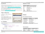
After EMSO is started a graphical user interface, as showed in
Figure 2.1, raises.
Note: The EMSO graphic interface layout and behavior is identical
in all platforms.
In this section a brief overview about this interface is given.
This interface is inspired on the most successfully interfaces for
software development. It is divided in some panels which are
treated in the following sections.

10 2 Overview
Figure 2.1: EMSO graphical user interface.
Explorer and Results Windows
The Explorer and Results windows are in the left most
vertical frame of the interface in Figure 2.1.
Explorer :
Results :
displays the available libraries of models and the current
loaded files and its contents (Models and FlowSheets).
The Figure 2.2 (a) shows a typical view of the file explorer.
for each task ride (e.g. a dynamic simulation) a new item is
added to this window. A typical view of the results explorer
can be seen in Figure 2.2 (b).
Tip: The position of the frames in Figure 2.1 can be freely interchanged,
right click on the tab button of the window to change
its position.
Each of these windows can be turned the current one by clicking
in the respective tab. At any time the user can close one or more
tabs. Closed tabs can be shown again with the View menu.
Problems Window
As in any programming or description language files can have
problems. Each time that a file is opened the Problems window
automaticaly list all errors and warnings found, as exemplified by
the Figure 2.3.

2.4 Tutorials 11
(a) Explorer
(b) Results explorer
Figure 2.2: EMSO Explorer and Results windows.
Figure 2.3: EMSO Problems Window.
Console Window
The Multiple Document Interface panel
When running tasks all messages are sent to the Console. As
can be seen in Figure 2.4, the user can select the detailing level
of the messages sent to the console.
In the center of the interface is implemented a Multiple Document
Interface (MDI) panel. This panel is responsible to show the
opened files and edit it, the result plots, etc.
2.4 Tutorials
In the last section we have presented how to start EMSO and its
graphical interface. Now we give some tutorials introducing the
key concepts of EMSO and its modeling language. The directory

12 2 Overview
Figure 2.4: EMSO Console Window.
/mso/tutorial/ contains all code samples found in
this section, where is the directory where EMSO was
installed.
2.4.1 Three Tank FlowSheet
In this section we describe how to create and simulate the dynamic
model of a process composed by some tanks. The example
consists of three tanks connected in series. In EMSO this process
can be modeled as a FlowSheet containing three Devices
each one based on a tank Model.
Creating a new file
In order to simulate this example, the first step is to create a new
.mso file containing a FlowSheet. This is achieved by left
clicking in the new file button . This will bring up the new file
dialog as shown in Figure 2.5. In this window the user can select
one of the available templates:
• FlowSheet;
• Equation FlowSheet;
• Model;
• Empty.
In this example we are interested in create a new FlowSheet.
This is the default template item, therefore the user should left it
as is. The fields Name and Location should be filled with the
desired file name and directory location, respectively. The user
can fill this dialog as exemplified in Figure 2.5 then left click in
the Accept button in order to create the new file. After this
EMSO will create and open a file with the given properties. At
this point the interface will look like Figure 2.6.

2.4 Tutorials 13
Figure 2.5: New file dialog wizard.
Figure 2.6: EMSO new file window.
Writing the FlowSheet
Before continue reading this tutorial is advisable to read the comments
on the file new file created (which comes from the selected
template).
The first comments are about the using command. This command
makes available all entities contained in a given filename or
directory (all files belonging to it).
In our example we will make use of one of the EML models, the
TankSimplified model. This model is found in file tanks.mso
in the library directory. Therefore, in order to use this model instead
of copy and paste we will use this file with the using
command as follows:
using "stage_separators/tanks";

14 2 Overview
The file tank.mso (as most of the
EML files) uses the file
types.mso which contains the
declaration of several variable types
as length, area, etc.
This command turns available all entities contained in file tank.mso
which is part of EML. For more details about using see subsection
3.1.5.
The next step is to change the default name NewFlowSheet
to a more meaningful name, lets say ThreeTank. Then we can
add the Devices in the DEVICES section and connect them in
the CONNECTIONS section. After this, the contents of the file
should look like Code 2.1.
Code 2.1: File ThreeTank1.mso.
17 using "stage_separators/tank";
19 FlowSheet ThreeTank
20 VARIABLES
21 Feed as flow_vol;
23 DEVICES
24 Tank1 as tank_simplified;
25 Tank2 as tank_simplified;
26 Tank3 as tank_simplified;
28 CONNECTIONS
29 Feed to Tank1.Fin;
30 Tank1.Fout to Tank2.Fin;
31 Tank2.Fout to Tank3.Fin;
32 end
The Code 2.1 contains no problems, once there is no item on the
Problems window.
Warning: Even if a .mso file has no problems the FlowSheets
of such file can be not consistent, as explained in the following
section.
Checking consistency
A FlowSheet is consistent if it has zero degrees of freedom and
zero dynamic degrees of freedom.
In order to check the ThreeTank consistency the user should
select the corresponding FlowSheet item in the file explorer
and then left click in the button. At this time the Console
window will become active and will display a message like:
Checking the consistency for ’ThreeTank’ in file ’
ThreeTank1.mso’...
Number of variables: 7
Number of equations: 6
Degrees of freedom: 1

2.4 Tutorials 15
The number of variables and equations does not match
!
System is not consistent!
At this point the Problems window will also show the consistency
problems. This error was expected, once we have neither
specified the input flow of the first tank nor the initial level of the
tanks.
Therefore, in order to get a consistent system the user should add
the following commands:
SPECIFY
Feed = 10 * ’mˆ3/h’;
INITIAL
Tank1.h = 1 * ’m’;
Tank2.h = 2 * ’m’;
Tank3.h = 1 * ’m’;
The user can choose between to add this code into its FlowSheet
or use the already made file ThreeTank2.mso found in the
tutorial directory.
Note: EMSO is not a sequential tool, therefore the user could
specify a variable other than the input flow of the first tank.
Now, if the user checks the ThreeTank consistency no errors
will be reported and some interesting messages will be sent to the
Console:
Checking the consistency for ’ThreeTank’ in file ’
ThreeTank2.mso’...
Number of variables: 10
Number of equations: 10
Degrees of freedom: 0
Structural differential index: 1
Dynamic degrees of freedom: 3
Number of initial Conditions: 3
System is consistent.
Running a Simulation
Once we have a consistent FlowSheet we can run a simulation.
To do this the user has to select the desired FlowSheet in the
file explorer and then left click in the button.
Simulation of ’ThreeTank’ started ...
Simulation of ’ThreeTank’ finished succesifuly in
0.02 seconds.

16 2 Overview
Tip: In order to get more detailed output when running a simulation
just change the output level on the Console window and
run again the simulation.
Visualizing Simulation Results
For each task ride by the user a new result is added to the results
explorer. The user can see the available results by left clicking in
the results explorer tab (Figure 2.2 (b)).
If a result is selected on the top list of the results, the bottom
side will show the variables available for plotting. The user can
plot a variable profile by double clicking in it.
We have not configured the simulation time vector for our simulation
and the default integration interval is not suitable for the
If not specified the integration
interval is the interval ranging from
dynamics of our system. We can modify the integration interval
0 to 100 seconds.
by adding, for instance, the following commands:
OPTIONS
TimeStep = 0.1;
TimeEnd = 2;
TimeUnit = ’h’;
Customizing the FlowSheet
Now we have an integration interval compatible with the dynamics
of our system. Then if we run the simulation again, the results
will be much more interesting.
Usually Models are full of parameters to be customized by the
user. In our FlowSheet (Code 2.1) we have not changed parameter
values. Hence the default values for all parameters were
considered, these defaults come from the types on which the parameters
are based.
In order to set values other than the defaults the user can add a
SET section at any point after the parameter declaration. Then
if we want another values for the valve constants or geometry of
our tanks the following code should be added after the DEVICES
section:
SET
Tank2.k = 8*’mˆ2.5/h’;
Tank2.A = 4*’mˆ2’;
Now we can run the simulation again and compare the results
with the previous solution.

2.4 Tutorials 17
At this point our code should look like Code 2.2 found in the
tutorial directory.
Code 2.2: File ThreeTank3.mso.
17 using "stage_separators/tank";
19 FlowSheet ThreeTank
20 VARIABLES
21 Feed as flow_vol;
23 DEVICES
24 Tank1 as tank_simplified;
25 Tank2 as tank_simplified;
26 Tank3 as tank_simplified;
28 CONNECTIONS
29 Feed to Tank1.Fin;
30 Tank1.Fout to Tank2.Fin;
31 Tank2.Fout to Tank3.Fin;
33 SPECIFY
34 Feed = 10 * ’mˆ3/h’;
36 INITIAL
37 Tank1.h = 1 * ’m’;
38 Tank2.h = 2 * ’m’;
39 Tank3.h = 1 * ’m’;
41 SET
42 Tank2.k = 8 * ’mˆ2.5/h’;
43 Tank2.A = 4 * ’mˆ2’;
45 OPTIONS
46 TimeStep = 0.1;
47 TimeEnd = 2;
48 TimeUnit = ’h’;
49 end

3 EMSO Modeling Language
In this chapter, we describe in detail how one can write a Model or FlowSheet using the
EMSO modeling language.
The EMSO modeling language is a case sensitive textual language. In such language the
entities are written in plain text files stored, by default, in .mso files.
Contents
3.1 Modeling basics . . . . . . . . . . . . . . . . . . . . . . . . . . . . 19
3.2 Model . . . . . . . . . . . . . . . . . . . . . . . . . . . . . . . . . . 23
3.3 FlowSheet . . . . . . . . . . . . . . . . . . . . . . . . . . . . . . . 28
3.4 Optimization . . . . . . . . . . . . . . . . . . . . . . . . . . . . . . 30
3.5 Built-in Functions . . . . . . . . . . . . . . . . . . . . . . . . . . . 35
3.6 Units Of Measurement (UOM) . . . . . . . . . . . . . . . . . . . . 36
3.7 Solver Options . . . . . . . . . . . . . . . . . . . . . . . . . . . . . 40
18

3.1 Modeling basics 19
3.1 Modeling basics
3.1.1 Object Oriented Modeling
Composition
Inheritance
As mentioned before, in EMSO a FlowSheet is the problem
in study. But, a FlowSheet is composed by a set of connected
Devices, each one having a mathematical description
called Model.
In chapter 2 the Model and FlowSheet entities were introduced.
The description of these entities share several basic concepts
particular to the EMSO modeling language, which follows.
Reuse is the key to handle complexities, this is the main idea behind
the object oriented (OO) paradigm. The EMSO language
can be used to create high reusable models by means of composition
and inheritance OO concepts, described below.
Every process can be considered as set of sub-processes and so
on, this depends only on the modeling level. Composition is the
ability to create a new model which is composed by a set of
components, its sub-models.
The EMSO modeling language provides unlimited modeling levels,
once one model can have sub-models which can have sub-models
themselves. This section aims at introducing the composition
concept, the application of this concept in the EMSO is shown in
subsection 3.2.3.
When modeling complex systems, set of models with a lot in
common usually arises. If this is the case, an advisable modeling
method is to create a basic model which holds all the common
information and derive it to generate more specif models reusing
already developed models.
In OO modeling this is achieved by inheritance, the ability to create
a new model based on a preexistent one and add derivations
to it. For this reason, inheriting is also known as deriving. When
a model uses more than one base model it is said to use multiple
inheritance.
See the EML file stream.mso, for
instance.
The EMSO modeling language provides unlimited levels of inheritance
or multiple inheritance for Models and FlowSheets.
The following sections and EML are a good sources of examples
of inheritances.

20 3 EMSO Modeling Language
3.1.2 Writing EMSO Entities
The basic EMSO entities are Models and FlowSheets. The
formal description of these entities always start with the entity
keyword (Model or FlowSheet) and ends with the end keyword,
as follows.
FlowSheet FlowSheetName
# FlowSheet body
end
Model ModelName
# Model body
end
3.1.3 Documenting with Comments
A .mso file can have an unlimited number of entities declared
on it. Once a entity was declared it is available to be used as
a base for derivation or as a component to another Model. The
detailed description of FlowSheets and Model are found in
sections 3.2 and 3.3, respectively.
The EMSO modeling language is a descriptive language, a Model
written on it contains several information about the process being
modeled, as variable and parameter description, equation names,
etc. But extra explanations could be useful for better understanding
the model or for documenting the history of a model,
the authors, the bibliography, etc. This kind of information can be
inserted in EMSO entities with one of the two types of comments
available:
• line comment: starting from # and extending until the end
of line;
• block comment: starting from #* and extending until *#.
It follows below a piece of code which exemplifies both kind of
comments:
#*
This is a block comment, it can be extended in
multiple lines.
A block comment can give to the reader useful
informations,
for instance the author name or a revision history:
Author: Rafael de Pelegrini Soares
---------------------------------------------------
Revision history

3.1 Modeling basics 21
$Log: streams.mso,v $
Revision 1.1.1.1 2003/06/26 16:40:37 rafael
---------------------------------------------------
*#
# A line comment extends until the end of line.
3.1.4 Types
As already mentioned in chapter 2, the declaration of variables
and parameters can make use of a base type. A type can be one
of the built-in types or types derived from the built-in ones. The
list of built-in types are shown in Table 3.1.
Table 3.1: List of EMSO built-in types.
Type name
Real
Integer
Switcher
Boolean
Plugin
Description
Type for continuous variables or parameters, with attributes:
• Brief: textual brief description
• Default: default value for parameters and initial guess for variables
• Lower: lower limit
• Upper: upper limit
• Unit: textual unit of measurement
Type for integer variables or parameters, with attributes:
• Brief: textual brief description
• Default: default value for parameters and initial guess for variables
• Lower: lower limit
• Upper: upper limit
Type for textual parameters, with attributes:
• Brief textual brief description
• Valid the valid values for the switcher
• Default default value for the switcher
Type for logical parameters or variables, with attributes:
• Brief textual brief description
• Default default value for parameters and initial guess for variables
Object for loading third party pieces of software providing special calculation
services, see chapter 5.

22 3 EMSO Modeling Language
As Table 3.1 shows, each built-in type has a set of attributes.
These attributes can be modified when a new type is created
deriving a preexistent one. For instance, consider the Code 3.1
making part of EML, in this file a set of convenient types are
declared, and are used in all EML models.
38 # Pressure
Code 3.1: EML file types.mso.
39 pressure as Real (Brief = "Pressure", Default=1,
Lower=1e-30, Upper=5e7, final Unit = ’atm’);
40 press_delta as pressure (Brief = "Pressure
Difference", Default=0.01, Lower=-5e6);
41 head_mass as Real (Brief = "Head", Default=50, Lower
=-1e6, Upper=1e6, final Unit = ’kJ/kg’);
42 head as Real (Brief = "Head", Default=50, Lower=-1e6
, Upper=1e6, final Unit = ’kJ/kmol’);
3.1.5 Using files
Note that type declarations can be stated only outside of any
Model or FlowSheet context.
Variables can be only declared based on types deriving from
Real. Note that the Plugin type cannot be derived to a new
type, read more in chapter 5.
Code reuse is one of the key concepts behind EMSO. To achieve
this the user can be able to use code written in another files
without have to touch such files. A .mso file can make use of
all entities declared in another files with the using command.
This command has the following form:
using "file name";
where "file name" is a textual file name. Therefore, commands
matching this pattern could be:
1 using "types";
2 using "streams";
3 using "tanks";
When EMSO find a using command it searches the given file
name in the following order:
1. the current directory (directory of the file where the using
was found);
2. the libraries configured on the system;

3.2 Model 23
Note: As shown in the sample code, if the user suppress the file
extension when using files EMSO will automatically add the
mso extension.
Whenever possible the user should prefer the using command
instead of copy and paste code.
Windows note: The EMSO language is case sensitive but the
windows file system is not. Therefore, when using files in windows,
the language became case insensitive to the file names.
3.2 Model
The basic form of a Model was introduced in subsection 3.1.2,
here we describe how the Model body is written.
In Code 3.2 the syntax for writing Models in the EMSO modeling
language is presented.
1 Model name [as base]
2 PARAMETERS
Code 3.2: Syntax for writing Models.
3 [outer] name [as base[( (attribute = value)+ )]
];
5 VARIABLES
6 [in | out] name [as base[( (attribute = value)+ )
] ];
8 EQUATIONS
9 ["equation name"] expression = expression;
11 INITIAL
12 ["equation name"] expression = expression;
14 SET
15 name = expression;
16 end
where the following conventions are considered:
• every command between [ ] is optional, if the command
is used the [ ] must be extracted;
• the operator ( )+ means that the code inside of ( )
should be repeated one or more times separated by comma,
but without the ( );

24 3 EMSO Modeling Language
• the code a|b means a or b;
• name is a valid identifier chosen by the user;
• base is a valid EMSO type or already declared Model;
• expression is an mathematical expression involving any
constant, variable or parameter already declared.
Therefore, using this convention, the the line 1 of Code 3.2 could
be any of the following lines:
Model MyModel
Model MyModel as BaseModel
Model MyModel as Base1, Base2, Base3
As another example, consider the line 5 of Code 3.2, commands
matching that pattern are:
MyVariable;
in MyVariable;
out MyVariable;
MyVariable as Real;
MyVariable as Real(Default=0, Upper = 100);
MyVariable as MyModel;
3.2.1 Parameters
When running an optimization or
parameter estimation the value of a
parameter could be the result of
the calculation.
Models of physical systems usually relies in a set of characteristic
constants, called parameters. A parameter will never be the result
of a simulation, its value needs to be known before the simulation
starts.
In Code 3.2, each identifier in capitals starts a new section. In
line 2 the identifier PARAMETERS starts the section where the
parameters are declared. A parameter declaration follows the pattern
shown in line 3, this pattern is very near to that used in type
declarations (see subsection 3.1.4).
In a Model any number of parameters, unique identified with
different names, can be declared. Examples of parameter declarations
follows:
PARAMETERS
NumberOfComponents as Integer(Lower=0);
outer OuterPar as Real;

3.2 Model 25
Outer Parameters
3.2.2 Variables
As can be seen in line 3 of Code 3.2 a parameter declaration
can use the outer prefix. When a parameter is declared with
this prefix, the parameter is only a reference to a parameter with
same name but declared in an outer context, for instance in a
FlowSheet. Because of this, parameters declared with the
outer prefix are known as outer parameters, while parameters
without the prefix are known as concrete parameters.
The purpose of outer parameters is to share the value of a parameter
between several Devices of a FlowSheet. Note that the
value of an outer parameter comes from a parameter with same
name but declared in some outer context. When the source of an
outer parameter is a FlowSheet its value is specified only in
the FlowSheet and then all models can use that value directly.
Every mathematical model has a set of variables once the variable
values describe the behavior of the system being modeled. These
values are the result of a simulation in opposition to parameters,
which need to be known prior to the simulation.
In the EMSO modeling language, variables are declared in a manner
very close to parameters. The VARIABLES identifier starts
the section where the variables are declared, following the form
presented in line 5 of Code 3.2. Examples of variable declarations
follows:
VARIABLES
T as Real(Brief="Temperature", Lower=200,
Upper = 6000);
in Fin as FlowRate;
out Fout as FlowRate;
Inputs and Outputs
A Model can contain an unlimited number of variables, but a
Model with no variables has no sense and is considered invalid.
The user should already note that the declaration of types, variables
and parameters are very similar, using a name and optionally
deriving from a base. In the case of variables and parameters the
base can be one of the built-in types (see Table 3.1), types deriving
from the built-in ones or predeclared Models.
When declaring variables, the prefixes in and out can be used,
see line 6 of Code 3.2.

26 3 EMSO Modeling Language
Variables declared with the out prefix are called output variables,
while that declared with the in prefix are called input variables.
The purpose of these kind of variables is to provide connection
ports, enabling the user to connect output variables to input variables.
An output variable works exactly as an usual variable, but is available
to be the source of a connection. However, an input variable
is not a concrete variable, once it is only a reference to the values
coming from the output variable connected to it. This connecting
method is used, instead of adding new hidden equations for each
connection, with the intent of reduce the size of the resulting system
of equations. A description on how to connect variables can
be found in subsection 3.3.2.
3.2.3 Composition in Models
In subsection 3.1.1 the composition concept was introduced. In
the EMSO modeling language, to built composed Models is
nothing more than declare parameters or variables but using Models
as base instead of types.
If a Model is used as base for a variable such variable actually is
a sub-model and the Model where this variable was declared is
called a composed Model.
A variable deriving from a Model contains all the variables, parameters
even equations of the base. In order to access the the
internal entities of a sub-model, for instance in equations or for
setting parameters, a path should be used, as exemplified in line 4
of the code below:
1 VARIABLES
2 controller as PID;
3 SET
4 controller.K = 10;
In the case of parameters deriving from a Model, the inheriting
process has some peculiarities:
• Parameters of the base are sub-parameters;
• Variables of the base are considered as sub-parameters;
• Equations, initial conditions and all the rest of the base are
unconsidered;

3.2 Model 27
3.2.4 Equations
Equations are needed to describe the behavior of the variables of
a Model. A Model can have any number of equations, including
no equations. In EMSO an equation is an equality relation between
two expressions, it is not an attributive relation. Therefore,
the order in which the equations are declared does not matter.
Warning: A Model with more equations than variables is useless,
once there is no way to remove equations from a model.
An equation is declared using the form presented in line 7 of
Code 3.2, where expression is a expression involving any of
preciously declared variables, parameters, operators, built-in functions
and constants. A constant can be a number or the text of
a unit of measurement. Details about the available operators,
functions and their meaning can be found in section 3.5.
Examples of equation follows:
EQUATIONS
"Total mass balance" diff(Mt) = Feed.F - (L.F
+ V.F);
"Vapor pressure" ln(P/’atm’) = A*ln(T/’K’) + B
/T + C + D*Tˆ2;
Units of measurement
Note that ’atm’ and ’K’, in the code above, are not comments,
such texts are recognized as units of measurement (UOM) constants
and effectively are part of the expression. In such example
the UOMs are required to assure units dimension correctness, because
the ln function expects a UOM dimensionless argument.
The UOM of a variable or parameter comes from its type or
declaration, for example:
temperature as Real(final Unit=’K’, Lower = 100,
Upper = 5000);
pressure as Real(final Unit=’atm’, Lower = 1e-6,
Upper = 1000);
VARIABLES
T1 as temperature;
T2 as Real(Unit = ’K’);
P1 as pressure;
P2 as pressure(Unit = ’kPa’); # error because
Unit was declared as final in pressure
P2 as pressure(DisplayUnit = ’kPa’);

28 3 EMSO Modeling Language
3.2.5 Initial Conditions
An attribute of a type can be fixed with the final prefix. A final
attribute cannot be changed when deriving from it. In the above
code, the declaration of variable P2 contains an error because the
Unit attribute of pressure is final and cannot be changed.
Declaring Unit attributes as final is important because the
limits (Lower and Upper) are considered to be in the same
UOM as Unit. But making a Unit to be final still leaves
to the user the option to change the UOM to be displayed in results.
This can be achieved setting the DisplayUnit attribute
accordingly.
EMSO can execute dynamic and steady state simulations, see
subsection 3.3.4. Most dynamic systems requires a set of initial
conditions in order to obtain its solution. These initial conditions
are stated exactly as equations (subsection 3.2.4 but within the
INITIAL section identifier, for instance:
INITIAL
"Initial total mass" Mt = 2000 * ’kg’;
3.2.6 Abstract Models
Note that the ”equations” given in the INITIAL section are used
only in the initialization procedure of dynamic simulations.
If a Model has less equations than variables it is known as a rectangular
or abstract Model, because specifications, connections
or extra equations are required in order to obtain its solution. If
a Model has no equation it is known as a pure abstract Model,
once it holds no information about the behavior of its variables.
Most models of a library are abstract or pure abstract where the
pure abstract models are derived to generate a family of abstract
models and so on. Note that is very uncommon to have a pure
abstract model used directly in a FlowSheets as well as to use
a model which is not abstract.
3.3 FlowSheet
In section 3.2 the Model body was described. When writing
FlowSheets the user can freely make use of all description
commands of a Model body, exactly as stated in section 3.2.
Additionally, in the case of FlowSheets, the sections presented
in in Code 3.3 could be used.

3.3 FlowSheet 29
Code 3.3: Syntax for writing FlowSheets.
1 FlowSheet name [as base]
2 DEVICES
3 name [as base[( (attribute = value)+ )] ];
5 CONNECTIONS
6 name to name;
8 SPECIFY
9 name = expression;
11 OPTIONS
12 name = value;
13 end
3.3.1 Devices
Code 3.3 uses the same code conventions explained in section 3.2.
It follows below the details of the sections of this code.
In line 2 of the Code 3.3 the DEVICES section can be seen. In
this section the user can declare any number of Devices of a
FlowSheet, in OO modeling these Devices are known as the
components, see subsection 3.1.1.
The DEVICES section in a FlowSheet is a ”substitute” of the
VARIABLES section of a Model but no prefix is allowed.
Note: There is no sense in using the in or out prefix in
FlowSheets, because these supposed inputs or outputs could
not be connected once the FlowSheet is the top level model.
Exactly as variables of a Model, the base (line 3 of Code 3.3)
can be any a type, or Model.
Examples of Device declarations follows:
DEVICES
feed as MaterialStream;
pump1 as Pump;
pump2 as Pump;
3.3.2 Connections
In subsection 3.2.2 was described how to declare an input or output
variable. However, was not specified how to connect an output
variable to an input one. This can be done with the form
presented in line 6 of Code 3.3, where a output variable is connected
to an input.

30 3 EMSO Modeling Language
3.3.3 Specifications
3.3.4 Options
It is stressed that the values of an input variable are only references
to the values of the output connected to it avoiding extra
equations representing the connections and reducing the size of
the resulting system of equations.
Note that the CONNECTIONS section can be used in Models
in the same way that in FlowSheets. It was omitted when the
Model body was described on purpose because is more intuitive
to connect variables in a FlowSheet. There is no restrictions in
using connections in a Model, but, when possible, composition
and inheritance should be used instead.
In subsection 3.2.6 the term abstract model was defined, basically
it means models with missing ”equations”. Most useful models
are abstract, because of their flexibility. This flexibility comes
from the possibility of specify or connect the models in several
different fashions.
In order to simulate a FlowSheet it must have the number of
variables equal number of equations. FlowSheets using abstract
Models requires specifications for variables in the form
presented in line 9 of Code 3.3. In a specification expression
can be any expression valid for an equation (see subsection 3.2.4)
and name is the name or path name of the specified variable.
In order to adjust the simulation parameters of a FlowSheet
the user can make use of the OPTIONS section. The following
piece of code shows how to set simulation options of a FlowSheet:
OPTIONS
TimeStart = 1;
TimeStep = 0.1;
TimeEnd = 10;
TimeUnit = ’h’;
DAESolver( File = "dasslc");
In Table 3.2 all available options are listed.
3.4 Optimization
Optimization differ from simulation in several aspects. In simulation
problems the solvers will try to find the solution. In optimization
problems the solvers try to find the best solution with

3.4 Optimization 31
Table 3.2: FlowSheet options, default value in bold.
Option name Type Description
TimeStart real The reporting integration time start: 0;
TimeStep real The reporting integration time step: 10;
TimeEnd real The reporting integration time end: 100;
Dynamic boolean Execute dynamic or static simulation: true or false;
Integration text The system to be used in integration: "original",
"index1" or "index0";
RelativeAccuracy real The relative accuracy: 1e-3;
AbsoluteAccuracy real The absolute accuracy: 1e-6;
EventVarAccuracy real The independent variable accuracy when detecting state
events: 1e-2;
SparseAlgebra boolean To use sparse linear algebra or dense: true or false;
InitialFile text Load the initial condition from result file
GuessFile text Load the an initial guess from result file
NLASolver text The NLA solver library file name to be used:
"sundials", "nlasolver", or the name the file
of some solver developed by the user as described in
chapter 7;
DAESolver text The DAE solver library file name to be used:
"dasslc", "sundials", "dassl", "mebdf", or
the name the file of some solver developed by the user
as described in chapter 7;

32 3 EMSO Modeling Language
respect to some objectives and constraints. The objectives can
be to minimize or maximize one or more expressions.
EMSO can be used to execute optimizations ranging from simple
to large-scale. When writing optimization problems the user can
freely make use of all description commands of a FlowSheet
body, exactly as stated in section 3.3. Additionally, in the case
of optimization problems, the sections presented in in Code 3.4
could be used.
Code 3.4: Syntax for writing FlowSheets.
1 Optimization name [as base]
2 MINIMIZE
3 expression1;
4 expression2;
6 MAXIMIZE
7 expression3;
8 expression4;
10 EQUATIONS
11 expression5 < expression6;
12 expression7 > expression8;
14 FREE
15 variable1;
16 variable2;
17 end
3.4.1 Simple Optimizations
Code 3.4 uses the same code conventions explained in section 3.2.
It follows below the details of the sections of this code.
An example of simple optimization problem follows:
Optimization hs71
VARIABLES
x(4) as Real(Default=1, Lower=1, Upper=5);
MINIMIZE
x(1)*x(4)*(x(1)+x(2)+x(3))+x(3);
EQUATIONS
x(1)*x(2)*x(3)*x(4) > 25;
x(1)*x(1) + x(2)*x(2) + x(3)*x(3) + x(4)*x(4)
= 40;
end
OPTIONS
Dynamic = false;

3.4 Optimization 33
As can be seen in the code above, optimization problems support
inequality constraints which are not supported in Models or
FlowSheets.
In the example above, the optimization is self-contained. The
variables, optimization objectives and constraints are all declared
in the optimization problem body.
Tip: Optimization problems are solved exactly as FlowSheets,
with the run button.
3.4.2 Large-Scale Optimization
In subsection 3.4.1 we described how to write a simple optimization
problem. The same approach can be used to describe largescale
problems but this form is barely convenient.
As a convenience for the user, EMSO supports the directly optimization
of already running FlowSheets. As an example,
consider that the user has an already developed and running
FlowSheet for a process of ammonia synthesis called Ammonia.
Now lets consider that the user want to find the recycle fraction
which yields to the minimun lost of product on the purge. For
this case the following code could be used:
Optimization AmmoniaOptimization as Ammonia
MINIMIZE
productLoose;
FREE
Splitter102.fraction;
end
OPTIONS
Dynamic = false;
Warning: In order to optimize FlowSheets make sure that the
FlowSheet can run (it should be consistent and the simulation
should succed).
3.4.3 Options
In subsection 3.3.4 all options supported by FlowSheets were
presented. Optimization problems support additional options as
listed in Table 3.3.

34 3 EMSO Modeling Language
Table 3.3: Optimization options, default value in bold.
Option name Type Description
NLPSolveNLA boolean Flag if the simulation solution should be used as start
value for the optimization problem: true or false;
NLPSolver text The file name of the NLP solver library:
"ipopt emso", or the name the file of some
solver developed by the user as described in chapter 7;
3.4.4 Dynamic Optimization
Under construction: As of this time, EMSO only supports static
optimization, dynamic optimization will be available soon.

3.5 Built-in Functions 35
3.5 Built-in Functions
In this section the built-in functions supported by the EMSO are
listed. There are two categories of functions:
• Element-by-element: if the argument of the function is a
vector or matrix, the function is applied in the same way to
all elements of the argument. The returned value of these
functions always have the same dimensions of its argument;
• Matrix transformation: The functions in this category
make sense only for vector and matrix arguments. The
return value can be a scalar, vector, or matrix depending
on the function and the argument.
Examples of use of the functions are available in the folder
/mso/sample/miscellaneous.
Table 3.4: Element-by-Element functions.
Function Meaning
diff(Z) Returns the derivative of Z with respect to time
exp(Z) Returns the exponential function, e raised to the power Z
log(Z) Returns the base 10 logarithm of Z
ln(Z)
Returns the natural logarithm (base e) of Z
sqrt(Z) Returns the square root of Z
Trigonometric
sin(Z) Returns the sine of Z
cos(Z) Returns the cosine of Z
tan(Z) Returns the tangent of Z
asin(Z) Returns the angle whose sine is Z
acos(Z) Returns the angle whose cosine is Z
atan(Z) Returns the angle whose tangent is Z
Hyperbolic
sinh(Z) Returns the hyperbolic sine of Z
cosh(Z) Returns the hyperbolic cosine of Z
tanh(Z) Returns the hyperbolic tangent of Z
coth(Z) Returns the hyperbolic cotangent of Z
Discontinuous
abs(Z) Returns the magnitude or absolute value of Z
max(Z) Returns the maximum value of Z
min(Z) Returns the minimum value of Z
sign(Z) Returns the signal of Z (-1 if Z < 0 e 1 if Z> 0
round(Z) Returns the small integer value of Z

36 3 EMSO Modeling Language
Function
Sum
sum(VEC)
sum(MAT)
sumt(MAT)
Product
prod(VEC)
prod(MAT)
prodt(MAT)
Transpose
transp(MAT)
Table 3.5: Matrix Transformation Functions.
Meaning
Returns a scalar with the sum of all elements of the vector VEC
Returns a vector with the sum of each column of the matrix MAT
Returns a vector with the sum of each row of the matrix MAT
Returns a scalar with the product of all elements of the vector
VEC
Returns a vector with the product of each column of the matrix
MAT
Returns a vector with the product of each row of the matrix MAT
Returns the transpose of a matrix MAT
3.6 Units Of Measurement (UOM)
The units of measurement recognized by the EMSO modeling
language are listed below.
3.6.1 Fundamental Units
m
kg
s
K
A
mol
cd
rad
US$
length in meters
mass in kilogram
time in seconds
temperature in Kelvin
eletric current in Ampere
the amount of substance in mole
the luminous intensity in Candela
angle measure in radian
money in dollar (USA)
3.6.2 Derived Units
Acceleration of Gravity
ga 9.80665*m/s 2 std acceleration of gravity
Angle
arcs 4.8481368111e-6*rad arcsecond
arcmin 2.90888208666e-4*rad arcminute
grad 1.57079632679e-2*rad grad
deg 1.74532925199e-2*rad degree

3.6 Units Of Measurement (UOM) 37
Area
acre 4046.87260987*m 2 acre
a 100*m 2 are
ha 10000*m 2 hectare
b 1e-28*m 2 barn
Eletric
Wb kg*m 2 /A/s 2 weber
T kg/A/s 2 tesla
S A 2 *s 3 /kg/m 2 siemens
mho A 2 *s 3 /kg/m 2 mho
Fdy 96487*A*s faraday
F A 2 *s 4 /kg/m 2 farad
ohm kg*m 2 /A 2 /s 3 ohm
C A*s relative current for batteries
V kg*m 2 /A/s 3 volt
Energy
J kg*m 2 /s 2 joule
kJ 1e3*J kilojoule
MJ 1e6*J megajoule
GJ 1e9*J gigajoule
eV 1.60217733e-19*J electronvolt
MeV 1e6*eV megaelectronvolt
therm 105506000*J therm
Btu 1055.05585262*J British thermal unit
cal 4.1868*J calorie
kcal 1e3*cal kilo calorie
erg 1e-7*J erg
Force
N kg*m/s 2 newton
pdl 0.138254954376*N poundal
lbf 4.44822161526*N pounds of force
kip 4448.22161526*N kip
gf 0.00980665*N gram force
kgf 1e3*gf kilogram force
dyn 0.00001*N dyne
Length
cm 1e-2*m centimeter
mm 0.1*cm millimeter
fermi 1e-15*m fermi
Å 1e-10*m angstrom
µ 1e-6*m micro

38 3 EMSO Modeling Language
mil 2.54e-5*m mil
ftUS 0.304800609601*m international foot
fath 1.82880365761*m fathom
rd 5.02921005842*m rod
chain 20.1168402337*m chain
miUS 1609.34721869*m US statute miles
nmi 1852*m nautical mile
mi 1609.344*m International Mile
km 1000*m Kilometer
au 1.495979e11*m Astronomical Unit
lyr 9.46052840488e15*m light year
pc 3.08567818585e16*m parsec
Mpc 3.08567818585e22*m megaparsec
in 0.0254*m inch
ft 0.3048*m foot
yd 0.9144*m yard
Mass
u 1.6605402e-27*kg atomic mass unit
grain 0.00006479891*kg grain
ct 0.0002*kg carat
ozt 0.0311034768*kg troy ounce
t 1000*kg tonne
tonUK 1016.0469088*kg ton (UK)
ton 907.18474*kg ton
lbt 0.3732417216*kg troy pound
slug 14.5939029372*kg slug
oz 0.028349523125*kg ounce
lb 0.45359237*kg pound
g kg/1000 gram
kmol 1e3*mol kilomole
lbmol 453.59237*mol pound mole
Money
R$ US$/3.05 Brazilian money (Real)
Power
W kg ∗ m 2 /s 3 watt
kW 1e3*W Kilowatt
MW 1e6*W megawatt
hp 745.699871582*W horsepower
Pressure
Pa kg/m/s 2 pascal
kPa 1e3*Pa Kilopascal

3.6 Units Of Measurement (UOM) 39
MPa 1e3*kPa megapascal
inH2O 248.84*Pa inch of water column
inHg 3386.38815789*Pa inch of mercury
mmHg 133.322368421*Pa millimeter of mercury
torr 133.322368421*Pa torr
psi 6894.75729317*Pa pound per square inch
bar 1e5*Pa bar
atm 101325*Pa atmosphere
Radiation
R 0.000258*A*s/kg R
Ci 3.7e10/s curie
Bq 1/s becquerel
Sv m 2 /s 2 sievert
rem 0.01*m 2 /s 2 rem
Gy m 2 /s 2 gray
Temperature
degR K/1.8 degree Rankine
Time
Hz 1/s hertz
min 60*s minute
rpm 1/min revolution per minute
h 60*min hour
d 24*h day
yr 31556925.9744*s year
Velocity
c 299792458*m/s light speed
knot 0.514444444444*m/s knot
mph 0.44704*m/s mile per hour
kph 0.277777777778*m/s kilometer per hour
Viscosity
St 0.0001*m 2 /s stoke
P 0.1*kg/m/s poise
cP 0.001*kg/m/s centipoise
Volume
st m 3 Stere
fbm 0.002359737216*m 3 board foot
pk 0.0088097675*m 3 peck
bu 0.03523907*m 3 bushel
bbl 0.158987291928*m 3 barrel
trp 4.92892159375e-6*m 3 teaspoon
tbsp 1.47867647813e-5*m 3 tablespoon

40 3 EMSO Modeling Language
3.7 Solver Options
ozUK 2.8413075e-5*m 3 fluid ounce (UK)
ozfl 2.95735295625e-5*m 3 fluid ounce
cu 2.365882365e-4*m 3 US Cup
l 1e-3*m 3 liter
ml 1e-3*l milliliter
pt 0.000473176473*m 3 pint
qt 0.000946352946*m 3 quart
gal 0.00378541178*m 3 gallon
galC 0.00454609*m 3 imperial gallon
galUK 0.004546092*m 3 gallon (UK)
Solver specific options can be declared in the following way, they
are not case sensitive:
OPTIONS
Dynamic = false;
NLPSolveNLA = false;
NLPSolver(File = "ipopt_emso",
RelativeAccuracy = 1e-6, limited\_memory\
_max\_history = 20);

3.7 Solver Options 41
Table 3.6: IPOPT optimization solver specific options, default value in bold.
Option name Type Description
MaxIter integer Maximum number of iterations: textbf3000
Print level integer Output verbosity level. The valid range for this integer
option is 0 ≤ printlevel ≤ 11
Limited memory max history integer Maximum size of the history for the limited quasi-
Newton Hessian approximation. The valid range for this
integer option is 0 ≤ 6 < + ∞
Derivative test string Enable derivative checker: first-order,
second-order, none
Derivative test print all string Indicates whether information for all estimated derivatives
should be printed: yes, no
Output file string File name of desired output file. ipopt.out
Mu strategy string Update strategy for barrier parameter: "adaptive",
monotone
Print user options string Print all options set by the user: "yes", no
RelativeAccuracy real Desired convergence tolerance (relative): 1 · 10 −08
Acceptable tol real Acceptable” convergence tolerance (relative): 1 · 10 −06
Constr viol tol real Desired threshold for the constraint violation(Absolute):
1 · 10 −04
Acceptable constr viol tol real ”Acceptance” threshold for the constraint violation(Absolute):
1 · 10 −02
Dual inf tol real Desired threshold for the dual infeasibility(absolute): 1 ·
10 −04
Acceptable dual inf tol real ”Acceptance” threshold for the dual infeasibility(absolute):
1 · 10 −02
Barrier tol factor real Factor for mu in barrier stop test.(absolute): 1 · 10 +01
Compl inf tol real Desired threshold for the complementarity conditions:
1 · 10 −04

42 3 EMSO Modeling Language
Table 3.7: OPT++ optimization solver specific options, default value in bold.
Option name Type Description
MaxIterations integer Maximum number of iterations: 100
MaxFeval integer Maximum number of function evaluations allowed:
1000
MaxBTIter integer Maximum number of Back Track iterations allowed: 5
PrintDebug integer Print debug information: 1, 0
SearchStrategy string Search Strategy: BTLineSearch, TrustRegion,
LineSearch
MeritFun string Search Strategy: ArgaezTapia, NormFmu,
VanShanno ;
OutputFile string Output file name: opt.out
RelativeAccuracy real set the Function tolerance: 1.49 · 10 −08
GradTol real set the Function tolerance: 6 · 10 −06
ConstrTol real set the Function tolerance: √ eps
StepTol real set the Function tolerance: 1.49 · 10 −08
MaxStep real set the Function tolerance: 1 · 10 +03
MinStep real set the Function tolerance: 1.49 · 10 −08
LineSearchTol real set the Function tolerance: 1 · 10 −04
TRSize real set the Function tolerance: 0.1 ∗ ‖∇f(x)‖
Table 3.8: NLASolver and Sundials specific options, default value in bold.
Option name Type Description
MaxIterations integer Maximum number of iterations: 100
Maxatbound integer Maximum number of iterations at bound: 20
MaxDumpIter integer Maximum dump iteration: 6
MaxLSetupReuse integer Maximum Jacobian reuse in the linear solving phase: 0
RelativeAccuracy real set the Function tolerance: 1 · 10 −03
AbsoluteAccuracy real set the Function tolerance: 1 · 10 −06

3.7 Solver Options 43
Table 3.9: IDASolver specific options, default value in bold.
Option name Type Description
MaxIterations integer Maximum number of internal steps to be taken by the
solver in its attempt to reach tout. 500
MaxOrder integer Maximum LMM mathod order: 5
SuppressAlg integer Suppress alg. vars. from error test 0
RelativeAccuracy real Set the function tolerance: 1 · 10 −03
AbsoluteAccuracy real Set the function tolerance: 1 · 10 −06
Hinit real Initial step size 0
Hmax real Maximum absolute value of step size allowed 1 · 10 10
Nconfac real Factor in nonlinear convergence test for use during integration
1.0
Table 3.10: DASSLC specific options, default value in bold.
Option name Type Description
MaxIterations integer Maximum number of internal steps to be taken by the
solver in its attempt to reach tout. 10
MaxOrder integer Maximum LMM mathod order: 5
Maxl integer max. number of iterations before restart: 5
Kmp integer number of orthogonalized vectors: 5
Istall integer intermediate time steps : 5
RelativeAccuracy real Set the function tolerance: 1 · 10 −03
AbsoluteAccuracy real Set the function tolerance: 1 · 10 −06

4 Advanced Modeling
In chapter 3 the basic concepts of the EMSO modeling language were described.
chapter we describe more advanced concepts.
In this
Contents
4.1 Arrays . . . . . . . . . . . . . . . . . . . . . . . . . . . . . . . . . . 45
4.2 Conditional Modeling . . . . . . . . . . . . . . . . . . . . . . . . . 48
44

4.1 Arrays 45
4.1 Arrays
4.1.1 Vectors
In EMSO we can make use of multidimensional arrays, i.e., arrays
with any number dimensions.
The simplest form of an array is the one dimension array – a
vector. In EMSO a vector of variables is declared as follows:
PARAMETERS
N as Integer(Default=10);
VARIABLES
vector1(100) as Real(Brief="A vector with 100
elements");
vector2(N) as Real(Brief="Undefined length
vector");
In the code above two vectors were declared, vector1 has a
fixed length while vector2 has its length equal to N which can
be set after.
Note: In order to build more general models the user should
declare the dimensions of the arrays as parameters. Remember
that the dimension of an array must be an Integer.
Besides the default types, in EMSO the user can compose new
models using vectors of another models as follows:
using "stream";
Model Mixer
PARAMETERS
Ninputs as Integer(Brief="Number of inputs",
Default=2);
VARIABLES
Inlet(Ninputs) as stream;
Outlet
as stream;
In the piece of code above the Inlet is a vector of length
Ninputs in which each element is a stream. The parameter
Niputs can be set after in any point of a the Model or in
the FlowSheet, for example:
FlowSheet MixProcess
DEVICES
mix as Mixer;
s1 as stream;
s2 as stream;
s3 as stream;

46 4 Advanced Modeling
CONNECTIONS
s1 to mix.Inlet(1);
s2 to mix.Inlet(2);
s3 to mix.Inlet(3);
end
SET
mix.Ninputs = 3;
Warning: Differently from some popular programming languages
as C or C++ the elements of a vector or array starts from one
and not zero.
4.1.2 Multidimensional Arrays
A vector is an array with only one
dimension, see subsection 4.1.1
Arrays with more than one dimension are declared in an analogous
way to vectors :
VARIABLES
var2d(x,y) as Real(Brief="Array with 2
dimensions");
var3d(x,y,z) as Real(Brief="Array with 3
dimensions");
4.1.3 Equation Expansion
The loop for is treated in
subsection 4.1.5
In usual programming languages, when dealing with vectors or
arrays the user has to work with loops, like for or while. EMSO
also implements a loop for but it has a convenient mechanism
which automatically expand the equations avoiding the use of
loops in most situations.
Arrays with Identical Shapes
For instance, if we wants an equation telling that the composition
of an outlet stream is equal to the composition of an inlet stream:
EQUATIONS
Outlet.z = Inlet.z;
Then EMSO automatically expands the above equation by:
Outlet.z i = Inlet.z i , i = 1 : Ncomps

4.1 Arrays 47
Arrays and Scalars
If an expression involve one array and one scalar, then the scalar
is expanded to match the array dimensions. For example:
VARIABLES
ones(M,N)
EQUATIONS
ones = 1;
as Real;
Note: The above equation ones=1; actually accounts as M
times N equations.
4.1.4 Array Functions
Sum
EMSO implements some functions specially designed for handling
arrays.
The sum function sums the elements of a vector or array. For
example, if in a mixer model we want to calculate the resulting
outlet flow rate we could use:
Outlet.F = ∑ i
Inlet i .F
The above equation can be obtained by the last line of the following
model:
Model Mixer
PARAMETERS
Ninputs as Integer(Brief="Number of inputs");
VARIABLES
Inlet(Ninputs) as stream;
Outlet
as stream;
EQUATIONS
Outlet.F = sum(Inlet.F);
Note: If the argument of sum is a vector it will return a scalar,
but if the argument is an matrix (array with two dimensions) it
will return a vector with length equal to the number of lines of
the matrix.
In general sum makes the summation of the last dimension of the
argument. For instance, if we have:

48 4 Advanced Modeling
VARIABLES
var3d(x,y,z) as Real(Brief="Three dimensional
array");
var2d(x,y) as Real(Brief="Two dimensional
array");
EQUATIONS
var2d = sum(var3d);
In the equation above, each element of var2d contains the sum
of all elements of var3d over z, which is the last dimension. In
other words:
var2d x,y = ∑ z
var3d x,y,z
Prod
The prod function returns the productory of a vector or array.
The logic of prod is exactly the same presented above for the
sum function.
4.1.5 Loop For
Most equations involving arrays are more convenient handled by
automatic equation expansion, see subsection 4.1.3. But in some
rare situations the equation expansion cannot yield the desired
result and one or more for loops are needed.
The syntax of a for loop is the following:
EQUATIONS
for i in [1:Ncomps]
Outlet.z(i) = Inlet.z(i);
end
Note: The index i used by the for loop above does not need
to be declared and is valid only in the context of the loop.
The above equation also can be written in a more compact fashion:
EQUATIONS
Outlet.z([1:Ncomps]) = Inlet.z([1:Ncomps]);
4.2 Conditional Modeling
Under construction: needs to be documented

5 Calculation Object Interface
In this chapter, we describe how the Plugin paradigm can be used to load, at run time,
third party software within EMSO entities. In chapter 6 is explained how to implement a new
Plugin service.
Contents
5.1 Introduction . . . . . . . . . . . . . . . . . . . . . . . . . . . . . . 50
5.2 Using Plugins . . . . . . . . . . . . . . . . . . . . . . . . . . . . . 51
49

50 5 Calculation Object Interface
5.1 Introduction
5.1.1 What is Plugin
In this section we describe what is a Plugin and what it is good
for.
Plugin is an interfacing mechanism which enables the user to
load calculation services provided by third party software within
EMSO. Typical cases where using Plugins is advisable are when
the following calculations are required:
• Property based on correlations
• Thermo-physical properties
CFD is the acronym for
Computational Fluid Dynamics.
• CFD calculations for complex geometries
5.1.2 Why use a Plugin
5.1.3 The Plugin Basics
EMSO is an equation-based tool, therefore most type of mathematical
relations can be expressed directly as equations of a
Model using the EMSO modeling language. However, there are
some cases in which using equations is barely convenient. Typical
examples include:
• The relationship cannot be expressed in a closed algebraic
form without introducing many intermediate quantities with
no physical sense;
• The relationship requires lots of data parameters;
• Already exists well established software that provides the
required calculation;
• It is difficult to converge the problem without decoupling
the system.
Before showing how to use a Plugin, let’s introduce its basics:
• Any number of Plugins can be declared within an EMSO
entity (Model, FlowSheet, etc.). The declaration of a
Plugin is very near to a parameter declaration;
• Each Plugin provides a set of methods which are the
calculation routines available to be used in EMSO;
• Each method calculates one quantity (the output) for given
zero or more other quantities (the inputs).

5.2 Using Plugins 51
• The output of a method, as each of its inputs, can be a
scalar or a vector of Real, Integer or Boolean and
have an unit of measurement (enabling EMSO to automatic
handle the required unit of measurement conversions).
• Additionally, a method can provide partial derivatives of its
output with respect to all or some of its inputs.
• Each Plugin service is provided by one library file which
must be compatible with the Plugin interface specification
presented in section 6.1.
5.2 Using Plugins
5.2.1 Using Plugins in Models
Plugin is one of the EMSO
built-in types, as Real, Integer,
etc.
In this section we show how to use Plugins within some EMSO
entities.
As already mentioned, the declaration of a Plugin is very near
to a parameter declaration but using as base the EMSO builtin
type Plugin. In Code 5.1 a typical usage of the Plugin
paradigm can be seen.
Code 5.1: EML file streams.mso.
45 Model liquid_stream as stream
46 ATTRIBUTES
47 Pallete = false;
48 Brief = "Liquid Material Stream";
49 Info =
50 "Model for liquid material streams.
51 This model should be used only when the phase
of the stream
52 is known ’’a priori’’.";
54 PARAMETERS
55 outer PP as Plugin(Brief = "External Physical
Properties", Type="PP");
57 EQUATIONS
58 "Liquid Enthalpy"
59 h = PP.LiquidEnthalpy(T, P, z);
60 "Liquid stream"
61 v = 0;
62 end
Outer parameters were treated in
subsection 3.2.1.
The Code 5.1 makes part of EML, in line 55 of it a Plugin is
declared. As can be seen, it is declared with the outer prefix,
therefore it is only an reference to a entity with same name but
declared in the top level model, the FlowSheet.

52 5 Calculation Object Interface
A calculation library must be a
valid DLL (dynamic link library) or
a SO (shared library) file in win32
and posix platforms respectively.
In the case of a concrete Plugin (declared without the outer
prefix) the user must supply the corresponding calculation library
type and optionally supply arguments to create the object. A
sample declaration of a concrete Plugin follows:
PARAMETERS
PP as Plugin(Brief="Physical Properties Object",
Type="PP");
In this code, the object PP will be created using the type PP. The
available Plugin types are configured with help of the Plugins
Configuration dialog, as shown in Figure 5.1. This dialog is can
be reached by the menu Config→Plugins.
Figure 5.1: Plugins Configuration dialog.
Using the dialog shown in Figure 5.1, the user can register any
number of Plugin types, but each type needs a unique type
name. Each type is dynamic linked by EMSO with the given file.
In line 59 of Code 5.1 a Plugin method is called, as can be
seen, this methods requires three inputs:
• T temperature;
• P pressure;
• z molar composition vector.
The cited method returns the molar enthalpy of the liquid phase
of the mixture represented by PP.

5.2 Using Plugins 53
Note: EMSO will check the units of measurement of all Plugin
arguments, it also checks the units of the returned value.

II.
Programming Guide
54

6 Developing new Plugin Services
In this chapter, we describe how to develop a new Plugin service enabling to load external
software within EMSO entities. In section 5.2 the usage of the Plugin interface was described.
Note that the information presented here is not a required to use Plugins but to
develop new services.
Contents
6.1 Interface Specification . . . . . . . . . . . . . . . . . . . . . . . . . 56
6.2 Writing new Plugin Services . . . . . . . . . . . . . . . . . . . . 63
6.3 Documenting Plugin Services . . . . . . . . . . . . . . . . . . . . 64
55

56 6 Developing new Plugin Services
6.1 Interface Specification
6.1.1 Create Function
In order to implement a Plugin service one can use any of
the most common scientific programming languages. There are
template implementations available for C, C++ and Fortran, presented
in sections 6.2.1, 6.2.2 and 6.2.3 respectively. It follows
bellow the concepts behind the Plugin interface.
Note: The information presented here is not required to use
already made Plugins but to develop new services.
A Plugin provides a set of methods, each of which receive zero
or more inputs and returns one output. In order to implement
a library which provides such service, one must implement the
following functions:
• create: creates a new instance of the Plugin service
• check method: checks if a specific method exists and
returns the number of inputs and outputs
• method details: provides detailed information about a
specific method
• set parameter: function for setting a parameter of the
object
• calc: provides the calculation for a given method
• destroy: destroys an object instance created with the
create function
In the following subsections these functions are detailed described.
Note that, depending on the programming langued used to actually
implement the service, a prefix in the function names can
be required. For instance, when implemented in C, the create
function should be eo create. In Frotran, depending the compiler
it should be eo create. For more details check subsection
6.2.1, subsection 6.2.2, or subsection 6.2.3.
When a new EMSO task is started, like a dynamic simulation, for
each concrete Plugin declared, EMSO creates a new instance
of such object. In this creation procedure the create function
is called in order to load the instance specific data.
The create function has the following form:
create(objectHandler, retVal, msg)

6.1 Interface Specification 57
where the arguments are as described in Table 6.1.
Table 6.1: Arguments of the Plugin create function.
Argument name Type Description
objectHandler [out] integer Unique identifier of the object instance
created (will be used to identify
the instance in subsequent calls).
retVal [out] integer Return flag, see .
msg [out] text A text space where error messages
should be copied.
EMSO does not need to known what really happens in the create
function, but the expected behavior is:
• create the memory to some data structure which holds the
instance dependent data;
• if some error or warning has occurred set retVal accordingly
and copy a message to the msg
• return the memory address of the data structure (or an
integer which unique identifies it) in the objectHandler
As EMSO Models, a Plugin can have parameters. An example
could be the required precision to be used when calculating a
method. These parameters can be set as usuall in the Model,
for instance:
PARAMETERS
PP as Plugin(Brief="Physical Properties Object",
Type = "PP", VapourModel = "PR",
LiquidModel = "PR");
For each attribute given EMSO will make a call to the set parameter
function. The prototype of the set parameter function is as
follows:
set_parameter(objectHandler,
parameterName, valueType, valueLength,
values, valuesText,
retVal, msg)
where the arguments are as described in Table 6.2.
The expected behavior of the set parameter function is:

58 6 Developing new Plugin Services
Table 6.2: Arguments of the Plugin set parameter function.
Argument name Type Description
objectHandler [in] integer Identifier of the object instance coming
from the create function.
parameterName [in] text The name of the parameter to be set.
valueType [in] integer The type of the parameter (1 for
Real, 2 for Integer, 3 for
Boolean and 4 for text)
valueLength [in] integer The length of the value (1 if is a
scalar)
values [in] real vector The vector of values (empty if the
type is text)
valuesText [in] text vector The vector of values (empty if the
type is not text)
retVal [out] integer Return flag, see .
msg [out] text A text space where error messages
should be copied.
• Check if the given parameterName is a valid parameter,
otherwhise set retVal accordingly and copy a message to
msg
• If the parameter is valid, store it to be used later
6.1.2 Destroy Function
When a Plugin instance is created the create function is
called. Then, when the object is no longer used by EMSO it
is destroyed. In some point of the destruction procedure the
destroy function is called. This function has the following
form:
destroy(objectHandler, retVal, msg)
where the arguments are as described in Table 6.3.
The expected behavior of the destroy function is to release any
memory, close data banks, etc. regarding the given objectHandler.
6.1.3 Verification Functions
A priori, EMSO does not known what are the methods supplied
by a particular Plugin nor the number or kind of its inputs

6.1 Interface Specification 59
Table 6.3: Arguments of destroy function.
Argument name Type Description
objectHandler [in] integer Identifier of the object instance coming
from the create function.
retVal [out] integer Return flag, see .
msg [out] text A text space where error messages
should be copied.
and outputs. This information is obtained with the functions
check method and method details.
Basically, the former function is used to check the existence of a
method and has the following form:
check_method(objectHandler, methodName, methodID,
numOfInputs, numOfOutputs,
retVal, msg)
where the arguments are as described in Table 6.4.
Table 6.4: Arguments of check method function.
Argument name Type Description
objectHandler [in] integer Identifier of the object instance coming
from the create function.
methodName [in] text Name of the method being checked.
methodID [out] integer Unique identifier for the given method
name (will be used to identify the
method in subsequent calls).
numOfInputs [out] integer The number of expected inputs of the
method.
numOfOutputs [out] integer The number of outputs of the
method.
retVal [out] integer Return flag, see .
msg [out] text A text space where error messages
should be copied.
From the check method function the following behavior is expected:
• Check the existence of a given methodName, if the method
does not exist this should be reported copying some message
into error.

60 6 Developing new Plugin Services
• If the required method exists, return the number of inputs
and the number of outputs. Optionally, an unique identifier
for the method can be returned in methodID. Then EMSO
will use this identifier in subsequent calls, this procedure can
speed up the evaluation of the functions.
Upon the ascertain of a method existence with the check method
function, the method details function is used to obtain detailed
information about the method. This function has the following
form:
method_details(objectHandler, methodName, methodID,
numOfInputs, inputLengths, inputTypes
, inputUnits,
numOfOutputs, outputLengths,
outputTypes, outputUnits,
hasDerivatives,
retVal, msg)
where the arguments are as described in Table 6.5.
The purpose of the method details function is to provide
detailed information about the inputs and outputs of a specific
method. The expected behaviour is:
• Given the methodName (or the methodID previouslly returned),
set inputLengths, inputTypes and inputUnits.
• Given the methodName (or the methodID previouslly returned),
set outputLengths, outputTypes and outputUnits.
• If the method will provide calculation for the derivatives set
hasDerivatives to 1.
6.1.4 Calculation Function
Given the inputs, each Plugin method calculates one or more
outputs. This calculation is provided by the calc function. This
should be implemented by the service, it has the following form:
calc(objectHandler, methodName, methodID,
outputLength, numOfInputs, inputLengths,
totalInputLenth,
methodInputs, methodOutput,
error, warning)
where the arguments are as described in Table 6.6.
The expected behaviour for the calc function is:

6.1 Interface Specification 61
Table 6.5: Arguments of check inputs function.
Argument name Type Description
objectHandler [in] integer Identifier of the object instance coming
from the create function.
methodName [in] text Name of the method being checked.
methodID [in] integer Identifier of the method coming from
the check method function.
numOfInputs [in] integer The number of inputs of the method.
inputLengths [out] integer vector The length of each input.
inputTypes [out] integer vector The type of each input (1 for Real, 2
for Integer and 3 for Boolean).
inputUnits [out] text vector The unit of measurement of each input.
numOfOutputs [in] integer The number of outputs of the
method.
outputLengths [out] integer vector The length of each output.
outputTypes [out] integer vector The type of each output (1 for Real,
2 for Integer and 3 for Boolean).
outputUnits [out] text vector The unit of measurement of each output.
hasDerivatives [out] integer If the method provides analytical
derivatives calculation
retVal [out] integer Return flag, see .
msg [out] text A text space where error messages
should be copied.

62 6 Developing new Plugin Services
Table 6.6: Arguments of calc function.
Argument name Type Description
objectHandler [in] integer Identifier of the object instance coming
from the create function.
methodName [in] text Name of the method being checked.
methodID [in] integer Unique identifier of the
method name, coming from
check method.
numOfInputs [in] integer The number of inputs.
inputLengths [in] integer vector The length of each input.
totalInputLength [in] integer Total input length.
inputValues [in] real vector Vector containing the input values.
numOfOutputs [in] integer The number of outputs.
outputLengths [in] integer vector The length of each input.
totalOutputLength [in] integer Total output length.
outputValues [out] real vector Vector to put the calculated output
values.
calculeDerivatives [in] integer Flag if the method should calculate
the derivatives or not.
outputDerivatives [out] real vector Vector to put the calculated output
derivative values.
error [out] text A text space where error messages
should be copied.
warning [out] text A text space where warning messages
should be copied.

6.2 Writing new Plugin Services 63
• Given the methodName (or the methodID set previously)
and the inputValues, calculate the method and store
the results on outputValues.
• Additionally, if the method has implementation for the derivatives
and calculeDerivatives is not false, return the
value of the derivatives on outputDerivatives.
6.2 Writing new Plugin Services
6.2.1 Writing Plugin Services in Fortran
6.2.2 Writing Plugin Services in C
In this section we describe how to implement a new Plugin
service using the most common scientific programming languages.
As a base concept of the Plugin interface was stated that an
EMSO entity can have any number of Plugins (see ). Therefore,
multiple instances of a Plugin service can be active simultaneously.
If this is the case and the service being implemented
has instance dependent data, each Plugin instance should allocate
its own data. Unfortunately, dynamic memory allocation is
not a trivial task in Fortran then if the service being implemented
is intended to support multiple instances the user should consider
in using C or C++ or wrap his Fortran implementation using such
languages.
As mentioned in section 6.1, in order to implement a new Plugin
service some functions must be implemented. In file external object.f
found at interfaces directory a template implementation for
a Plugin service in Fortran is given.
The template file has the required function calling conventions,
besides several comments which helps the user in the task of
implementing a new service and creating the library.
As mentioned in section 6.1, in order to implement a new Plugin
service some functions must be implemented. In file external object.c
found at interfaces directory a template implementation for
a Plugin service in C is given. This file makes use of the interface
definitions declared at external object.h. Note that
the header file should not be modified by the user.
The template file has the required function calling conventions,
besides several comments which helps the user in the task of
implementing a new service and creating the library.

64 6 Developing new Plugin Services
6.2.3 Writing Plugin Services in C++
6.3 Documenting Plugin Services
As mentioned in section 6.1, in order to implement a new Plugin
service some functions must be implemented. When using C++,
this functions actually are member functions of a class. In file
external object.cpp, found at interfaces directory, a
template implementation for a Plugin service in C++ is given.
This file makes use of the interface definitions declared in file
external object.h. Note that the header file should not be
modified by the user.
The C++ template file has a skeleton implementation that should
be filled by the user, besides several comments which helps the
user in the task of implementing a new service and creating the
library. Actually, when implement a new Plugin services in C++
the user can choose between implement the interfaces exactly as
described in the C template file or to implement it as class. The
C++ template file uses the class approach.
VRTherm is a software for physical
properties prediction from VRTech
www.vrtech.com.br.
The software VRTherm is a typical example of Plugin. Its
documentation can be used as a base for developing the manual
for a new service.
Basicaly, a good Plugin documentation should include at least:
• how to install the service;
• how to use the service
– what is the File of the library;
– specify whether the service supports multiple instances
or not;
– valid parameters and its purposes;
– document the methods supplied by the service as well
as the inputs and outputs.

7 Developing new Solvers
In this chapter, we describe how to develop new solver services enabling to solve the problems
coming from the FlowSheets with custom solvers. These solvers are called external solvers
because they could be freely implemented by third parties and are implemented in a very
similar way to Plugins described in chapter 6.
Contents
7.1 NLA Solvers . . . . . . . . . . . . . . . . . . . . . . . . . . . . . . 66
7.2 DAE Solvers . . . . . . . . . . . . . . . . . . . . . . . . . . . . . . 72
7.3 Writing new Solver Services . . . . . . . . . . . . . . . . . . . . . 75
7.4 Documenting Solver Services . . . . . . . . . . . . . . . . . . . . . 76
65

66 7 Developing new Solvers
7.1 NLA Solvers
Nonlinear-algebraic (NLA) systems arise naturally from steadystate
mathematical models or in the initialization of dynamic
simulations. In order to obtain the numerical solution, EMSO
automatically converts this kind of problem into the following
formulation:
F (y) = 0, y l < y < y u (7.1)
where y is the vector of variables to solve, F (y) is the vector
of functions (the equations), y l and y u are the lower and upper
bounds, respectivelly.
In this section we describe how to implement a new solver for
systems as Equation 7.1.
When communicating to solvers EMSO acts as a server which give
informations about the problem being solved. For NLA problems
EMSO provides four functions to the solver:
• ResFn: returns the residuals for a given y
• LSetup: tells EMSO to update the Jacobian matrix ∂F/∂y
• LSolve: solves for x the linear system Ax = b for a given
b, where A is the Jacobian matrix ∂F/∂y
This operation is also known as the
GEMV BLAS operation
• LProd: makes the product y = αAx + βy, where A is
the Jacobian matrix, α and β are scalars, x and y are given
vectors.
7.1.1 Residuals Function
Using the functions provided by EMSO, a new NLA solver needs
to implement the following routines:
• create: creates a new instance of the NLA external solver
for a given problem structure;
• solve: solves the problem;
• destroy: destroy the external solver instance created
with the create function;
For any point y c which is not the solution of Equation 7.1 we will
have a residual:
F (y c ) = res (7.2)

7.1 NLA Solvers 67
EMSO can calculate the residuals vector res with the ResFn
function which has the following form:
ResFn(y, res, EMSOdata, retVal)
where the arguments are as in Table 7.1.
Table 7.1: Arguments of the ResFn function.
Argument name Type Description
y [in] real Vector with the current point for y
res [out] real Residuals vector, will be calculated as a function
of y.
EMSOdata - EMSO problem specific data (should not be
used by the solver).
retVal [out] integer Return flag, see .
7.1.2 Jacobian
Newton’s like methods can solve Equation 7.1 iteratively with
some modification of the following equation:
∂F
∂y (yn − y n+1 ) = −F (y n ) (7.3)
where ∂F/∂y is the Jacobian and F (y n ) is the residuals vector
(subsection 7.1.1).
Using Equation 7.3 to solve the problem the solver will need to
solve a linear systems of equations. This can be done directly by
EMSO with the LSolve function:
LSolve(x. b, EMSOdata, retVal)
where the arguments are as in Table 7.2.
Note: The LSolve function solves for x given a vector b, depending
on the implementation of the solver, b can be −F (y n )
or not.
It should be noted that the Jacobian is opaque to the solver. As
a consequence, EMSO can use efficient storage structures (dense
or sparse) and specific algorithms for solving the linear system
which are independent from the solver implementation.

68 7 Developing new Solvers
Table 7.2: Arguments of the LSolve function.
Argument name Type Description
x [out] real Vector with the solution of the linear system
b [in] real The independent vector b
EMSOdata - EMSO problem specific data (should not be
used by the solver)
retVal [out] integer Return flag, see .
The LSolve function solves the linear system using the Jacobian
of the system. But aiming at efficiency EMSO does not updates
the Jacobian matrix each time it solves the linear system. The
solver needs to explicitly tell EMSO to update the Jacobian with
the function LSetup:
LSetup(EMSOdata, retVal)
where the arguments are as in Table 7.3.
Table 7.3: Arguments of the LSetup function.
Argument name Type Description
EMSOdata - EMSO problem specific data (should not be
used by the solver)
retVal [out] integer Return flag, see .
7.1.3 Matrix Multiplication
As can be seen in Table 7.3 the LSetup function does not require
an input argument for y. EMSO uses the y values given at
the last call to ResFn (subsection 7.1.1), this method improve
the efficiency when calculating the Jacobian using automatic differentiation.
Some modifications of the Newton method may require addition
linear algebra operations using the Jacobian matrix. For these
cases, EMSO provides a general product function, as follows:
y = αAx + βy
where A is the Jacobian matrix, α and β are scalars, x and y are
given vectors.

7.1 NLA Solvers 69
Note: The LProd function considers that x and y are given
vectors, therefore x or y can be the current solution point or the
current vector of residuals, it is up to the designed of the solver.
Some codes may need a simplified version of the product, y =
αAx. This is easily achieved passing β equal zero to the function
LProd.
The LProd function has the following prototype:
LProd(alpha, x, beta, y, EMSOdata, retVal)
where the arguments are as in Table 7.4.
Table 7.4: Arguments of the LProd function.
Argument name Type Description
alpha [in] real Given scalar
x [in] real Given vector
beta [in] real Given scalar
y [inout] real Given vector, will hold the result of the operation
EMSOdata - EMSO problem specific data (should not be
used by the solver).
retVal [out] integer Return flag, see .
7.1.4 Create and Destroy Functions
EMSO can run concurrent simulations, and so, in order to support
this feature, a new solver instance is created for each new
simulation started. Each time EMSO needs a new solver it calls
the create function of the solver. As a consequence, each instance
of the solver should have its own memory space to avoid
conflicts when running concurrent simulations.
The create function should allocate any memory needed by the
solver. All allocated memory should be released by the destroy
function.
The create function has the following form:
create(solverID, numOfEqs, resFn, y0, ylb, yub,
EMSOdata, iopt, ropt, retVal, msg)
where the arguments are as described in Table 7.5.

70 7 Developing new Solvers
Table 7.5: Arguments of the NLA solver create function.
Argument name Type Description
solverID [out] integer Unique identifier of the solver instance created
(will be used to identify the instance in subsequent
calls).
numOfEqs [in] integer The number of equations of the system.
resFn [in] function Function that calculates the residuals of the
system.
y0 [in] real vector Initial values of the variables.
ylb [in] real vector Lower bound for the variables.
yub [in] real vector Upper bound for the variables.
EMSOdata [in] integer EMSO problem specific data (only to pass back
to resFn, lsetup and lsolve)
iopt [in] integer vector The vector of integer options, see .
ropt [in] real vector The vector of real options, see .
retVal [out] integer Return flag, see .
msg [out] text A text space where error messages should be
copied.
Warning: The solver should return a unique SolverID for each
call to create because this integer will be used to identify the
solver instance in subsequent calls to solve or destroy.
When EMSO does not need the solver anymore it calls the destroy
function on it:
destroy(solverID, retVal, msg)
where the arguments are as described in Table 7.6.
Table 7.6: Arguments of the NLA solver destroy function.
Argument name Type Description
solverID [in] integer Unique identifier of the solver instance (returned
by create).
retVal [out] integer Return flag, see .
msg [out] text A text space where error messages should be
copied.
Using the given solverID the solver should release any memory
associated with that solver instance.

7.1 NLA Solvers 71
7.1.5 Solve Function
Note: When using C or C++, an easy way to implement an
unique identifier for the solver is to create an structure or class
for the solver and return its address as the identifier. Then the
solver just needs to cast back the SolverId to get the address
of the structure.
Once the solver instace has been created (as described in subsection
7.1.4), EMSO will generate a call to the solve function
each time EMSO needs to solve the problem.
The solve function has the following form:
solve(solverID, numOfEqs, resFn, lsetup, lsolve,
y, ylb, yub, EMSOdata, rtol, atol,
iopt, ropt, retVal, msg)
where the arguments are as described in Table 7.10.
Table 7.7: Arguments of the NLA solver solve function.
Argument name Type Description
solverID [out] integer Unique identifier of the solver instance (returned
by create).
numOfEqs [in] integer The number of equations of the system.
resFn [in] function Function that calculates the residuals of the
system.
y [inout] real vector Initial values of the variables and the solution
at the end.
ylb [in] real vector Lower bound for the variables.
yub [in] real vector Upper bound for the variables.
EMSOdata [in] integer EMSO problem specific data (only to pass back
to resFn, lsetup and lsolve)
rtol [in] real The relative accuracy
atol [in] real The absolute accuracy (optionally a vector)
iopt [in] integer vector The vector of integer options, see .
ropt [in] real vector The vector of real options, see .
retVal [out] integer Return flag, see .
msg [out] text A text space where error messages should be
copied.
EMSO can call multiple times the solve function before destoying
it. Each time EMSO asks the solver to solve the problem a
initial guess y is given and the solution should be returned on the
same vector.

72 7 Developing new Solvers
Warning: The parameter rtol is always a real scalar but atol
can be a vector depending on the options at iopt.
7.2 DAE Solvers
Differential-algebraic equations (DAE) arise naturally from dynamic
modeling in several engineering areas.
Prior to a dynamic simulation, EMSO internally converts in memory
the given FlowSheet description to a general DAE system
in the following form:
F (t, y, y ′ ) = 0, y l < y < y u (7.4)
where t is the independent variable (usually the time), y is the
vector of variables, y ′ are the derivatives of y with respect to t
and F are the equations of the problem being solved.
In EMSO a DAE solver is supposed only to advance one step
forward in the solution of a problem. In other words, given a valid
t n , y n , y ′ n the DAE solver should only to advance one step to a
next solution t n+1 , y n+1 , y ′ n+1.
Note: The first solution t 0 , y 0 , y ′ 0 is obtained using a NLA solver
in the initialization step.
Between calls to the DAE solver EMSO checks if events have
happened and make proper reinitializations if needed.
In a very similar way to NLA solvers (section 7.1) EMSO provides
a set of services which give informations about the problem being
solved:
• ResFn: returns the residuals of Equation 7.4 for a given
t, y, y ′
• LSetup: tells EMSO to update the Jacobian matrices
∂F/∂y and ∂F/∂y ′
• LFactor: builds the iteration matrix c∂F/∂y + d∂F/∂y ′
• LSolve: solves for x the linear system Ax = b for a given
b, where A is the iteration matrix c∂F/∂y + d∂F/∂y ′
Using the functions provided by EMSO, a new DAE solver needs
to implement the following routines:

7.2 DAE Solvers 73
7.2.1 Create and Destroy Functions
• create: creates a new instance of the DAE external solver
for a given problem structure;
• step: takes one step forward in the solution or makes an
interpolation for a desired point;
• destroy: destroy the solver instance created with the
create function;
EMSO can run concurrent simulations, in order to do this a new
solver instance is created for each new simulation started. The
create function is responsible for creating a new instance of the
solver and has the following form:
create(solverID, numOfEqs, resFn,
indVar0, y0, yp0, variableIndexes,
EMSOdata, rtol, atol, iopt, ropt,
retVal, msg)
where the arguments are as described in Table 7.8.
Table 7.8: Arguments of the DAE solver create function.
Argument name Type Description
solverID [out] integer Unique identifier of the solver instance created
(will be used to identify the instance in subsequent
calls).
numOfEqs [in] integer The number of equations of the system.
resFn [in] function Function that calculates the residuals of the
system.
y0 [in] real vector Initial values of the variables y.
y0 [in] real vector Initial values of the variable derivatives y ′ .
variableIndexes [in] integer vector The index of each variable (only for high index
problems).
EMSOdata [in] integer EMSO problem specific data (only to pass back
to resFn, lsetup and lsolve)
rtol [in] real The relative accuracy
atol [in] real The absolute accuracy (optionally a vector)
iopt [in] integer vector The vector of integer options, see .
ropt [in] real vector The vector of real options, see .
retVal [out] integer Return flag, see .
msg [out] text A text space where error messages should be
copied.

74 7 Developing new Solvers
Warning: The solver should return an unique SolverID for
each call to create because this integer will be used to identify
the solver instance in subsequent calls to step or destroy.
When EMSO does not need the solver anymore it calls the destroy
function on it:
destroy(solverID, retVal, msg)
where the arguments are as described in Table 7.9.
Table 7.9: Arguments of the DAE solver destroy function.
Argument name Type Description
solverID [in] integer Unique identifier of the solver instance (returned
by create).
retVal [out] integer Return flag, see .
error [out] text A text space where error messages should be
copied.
Using the given solverID the destroy function should release
any memory associated with that solver instance.
Note: When using C or C++ an easy way to implement an
unique identifier for the solver is to create an structure or class
for the solver and return its address as the identifier. Then the
solver just needs to cast back the SolverId to get the address
of the structure.
7.2.2 Step Function
After created as described in subsection 7.1.4, each time EMSO
needs to solve the problem it will call the solve function.
The solve function has the following form:
solve(solverID, numOfEqs, resFn, lsetup, lsolve,
y, ylb, yub, EMSOdata, rtol, atol,
iopt, ropt, retVal, msg)
where the arguments are as described in Table 7.10.
EMSO can call multiple times the solve function before destoying
it. Each time EMSO asks the solver to solve the problem a

7.3 Writing new Solver Services 75
Table 7.10: Arguments of the NLA solver solve function.
Argument name Type Description
solverID [out] integer Unique identifier of the solver instance (returned
by create).
numOfEqs [in] integer The number of equations of the system.
resFn [in] function Function that calculates the residuals of the
system.
y [inout] real vector Initial values of the variables and the solution
at the end.
ylb [in] real vector Lower bound for the variables.
yub [in] real vector Upper bound for the variables.
EMSOdata [in] integer EMSO problem specific data (only to pass back
to resFn, lsetup and lsolve)
rtol [in] real The relative accuracy
atol [in] real The absolute accuracy (optionally a vector)
iopt [in] integer vector The vector of integer options, see .
ropt [in] real vector The vector of real options, see .
retVal [out] integer Return flag, see .
msg [out] text A text space where error messages should be
copied.
initial guess y is given and the solution should be returned on the
same vector.
Warning: The parameter rtol is always a real scalar but atol
can be a vector depending on the options at iopt.
7.3 Writing new Solver Services
In this section we describe how to implement a new solver services
for both NLA and DAE systems using the most common scientific
programming languages.
As cited before EMSO is able to run concurrent simulations.
Therefore, multiple instances of a external solver service can be
active simultaneously. Unfortunately, dynamic memory allocation
is not a trivial task in Fortran and is left as a challenge to the
user. As an alternative the user should consider in using C or
C++ or wrap his Fortran implementation using such languages.
7.3.1 Writing External Solver Services in Fortran
As mentioned in sections and 7.2, in order to implement a new
external solver service a set of functions must be implemented. In

76 7 Developing new Solvers
7.3.2 Writing External Solver Services in C
7.3.3 Writing External Solver Services in C++
7.4 Documenting Solver Services
files NLASolverTemplate.f and DAESolverTemplate.f
found at interfaces directory are given template implementations
for an external NLA and DAE solvers services in Fortran.
The template files has the required function calling conventions,
besides several comments which helps the user in the task of
implementing a new service and creating the library.
As mentioned in section 7.2, in order to implement a new external
solver service a set of functions must be implemented.
In file ExterSolverTpl.c found at interfaces directory
a template implementation for a external solver service in C is
given. This file makes use of the interface definitions declared at
ExternalSolver.h. Note that the header file should not be
modified by the user.
The template file has the required function calling conventions,
besides several comments which helps the user in the task of
implementing a new service and creating the library.
As mentioned in section 7.2, in order to implement a new external
solver service a set of functions must be implemented. When using
C++ this functions actually are member functions of a class.
In file ExternalSolverTlp.cpp found at interfaces directory
a template implementation for an external solver service
in C++ is given. This file makes use of the interface definitions
declared in file ExternlaSolver.h. Note that the header
file should not be modified by the user. When included in a
C++ file the ExternlaSolver.h, besides the C interfaces,
declares two C++ pure abstract class called NLASolverBase
and DAESolverBase.
The C++ template file has a skeleton implementation that should
be filled by the user, besides several comments which helps the
user in the task of implementing a new service and creating the
library. Actually, when implement solver services in C++ the user
can choose between implement the interfaces exactly as described
in the C template files or to implement a class deriving from the
given pure virtual classes as made in the C++ template file.
Under construction: To be documented.