CENG 120 Final Exam (Fall, 2001). Open book and notes. Time: 3 h ...

CENG 120 Final Exam (Fall, 2001). Open book and notes. Time: 3 h.
Scoring: 1. 40; 2. 10; 3. 40; 4. 55; 5. 7; 6. 8 (160 points total)
You can use MATLAB in whatever way that it may help you. Where MATLAB listings are requested, write out
clearly the statements that you have used. If you want to print them out instead, collect all of them in one file first;
do not print them out individually.
1. Consider a simple unity feedback system with the following closed-loop characteristic equation:
1 +K c 1+ 1
5s
2
(s+1)(2s+1) =0
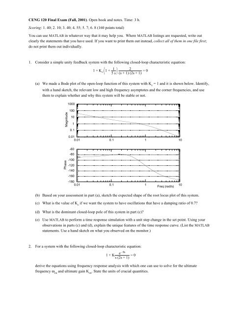
(a) We made a Bode plot of the open-loop function of this system with K c
= 1 and it is shown below. Identify,
with a hand sketch, the relevant low and high frequency asymptotes and the corner frequencies, and use
them to explain whether and why this system will be stable or not.
Magnitude
1000
100
10
1
0.1
0.01
0.01 0.1 1 10
Phase
-60
-80
-100
-120
-140
-160
-180
0.01 0.1 1
Freq (rad/s)
10
(b) Based on your assessment in part (a), sketch the expected shape of the root locus plot of this system.
(c) What is the value of K c
if we want the system to have oscillations that have a damping ratio of 0.7
(d) What is the dominant closed-loop pole of this system in part (c)
(e) Use MATLAB to perform a time response simulation with a unit step change in the set point. Using your
observations in parts (c) and (d), explain the unique features of the time response curve. (List the MATLAB
statements. Use a hand sketch on what you observed on the monitor.)
2. For a system with the following closed-loop characteristic equation:
e–
θs
1 +K
s(2s+1) =0
derive the equations using frequency response analysis with which one can use to solve for the ultimate
frequency ω cu
and ultimate gain K cu
. State the units of crucial quantities.

3. A control system is shown in the block diagram below. It uses a proportional controller and cascade rate
feedback of the manipulated variable.
R
+
–
K c
+
–
1
2s + 1
1
s
C
K 2
(a) For simplicity, take the primary controller gain K c
to be 1. What is the value of the rate feedback gain K 2
that may allow us to have a system response with a damping ratio of 1/√2
(b) With K c
= 1 and the value of K 2
obtained in part (a), hand sketch the root locus plot of the system.
(c) If we want to sketch the root locus plot of the system while holding K c
constant but varying K 2
as the
parameter, how would we do it What is the probable shape of this root locus plot if K c
= 1 (Hint: We
want to rearrange the closed-loop equation to the form: 1 + K 2
G(s) = 0.)
(d) What is the offset of the system
(e) Under what circumstance is this system stable with respect to K 2
> 0
(f) Do a MATLAB simulation of the closed-loop response with a unit step change in the set point using K c
= 1
and the value of K 2
obtained in part (a). (Write out your statements and provide a print out with your
solution.)
4. Consider a pressure control loop shown on the right. The
system makes use of the gas inlet stream to maintain a certain
pressure in the vessel. The control loop has a pressure
transducer and a controller that sends out a current signal to a
current-to-pressure converter. The I/P converter in turn drives
a pneumatic valve which manipulates the inlet stream flow.
The transfer functions for the pressure vessel and the
pneumatic valve are:
G p =
0.2
(0.2s + 1) (0.75s + 1)
PC
I/P
psi
scfm , and G v =
± 3
(0.1s + 1)
Inlet Stream
scfm
psi
PT
Outlet Stream
The choice of the action of the valve (i.e., the sign of the steady state gain) is to be determined later. Here we
use American engineering units. So gas flow is in scfm and pressure is in psi. The response of the pressure
transducer is extremely fast such that we can neglect its dynamics. It is calibrated for a pressure range of 0 to 30
psi with an output of 4-20 mA. The I/P converter takes in a 4-20 mA input and transmits it as 3-15 psi signal to
the pneumatic valve.
(a) We want to design a fail-closed system. Provide the action of each block (i.e., the sign of the steady state
gain in each block). Draw and label properly with units the block diagram of the system and identify the
sign of the steady state gain in each block, including the controller.
(b) Write down the closed-loop characteristic equation of the system with proper numerical values for all the
steady state gains.
(c) Using either the Routh array or direct substitution (entirely your choice), find the range of proportional gain
that a system with a proportional controller is stable.
(d) For a system with only proportional control, find the ultimate gain with a method of your choice.

(e) For a system with only proportional control, find the proportional gain when the system performance has
oscillations that are equivalent to a damping ratio of 0.7. Identify the dominant pole(s) in this case.
(f) What is the steady state error in part (e)
(g) For a system with only proportional control, find the proportional gain such that the system has a gain
margin of 2. List the MATLAB statements with which you use to calculate this result.
(h) Use direct synthesis to design a controller such that the system response has a damping ratio of 0.7.
(i) Suppose we now do an open-loop step test. On a single plot, compare the full-order model with the firstorder
with dead time approximation for the process reaction curve function. (Provide the statements and the
plot.)
(j) On a single plot, compare the closed-loop time responses to a unit step input with different PID controller
settings: (1) Ziegler-Nichols with slight overshoot, (2) ITAE, (3) direct synthesis from part (h), (4) IMC,
and (5) Ciacone-Marlin. Use an ideal PID controller in your simulation. (List clearly the controller settings
that you use and the MATLAB statements common to all different cases. Provide a copy of the plot.)
5. Show that with a proper choice of K 2
, the following two block diagrams are identical.
(a)
R + 1
C
K c
–
s (2s + 1)
(1 + τ s)
D
(b)
R + + 1 C
K c
–
– s (2s + 1)
K 2
s
6. If the poles of a transfer function are –2 ± j2√3, what are the natural time period and damping ratio of this
transfer function