Miscellaneous notes on mass transfer coefficient models

P.C. Chau (UCSD, 1999)
_____________
Appendix
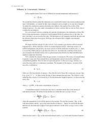
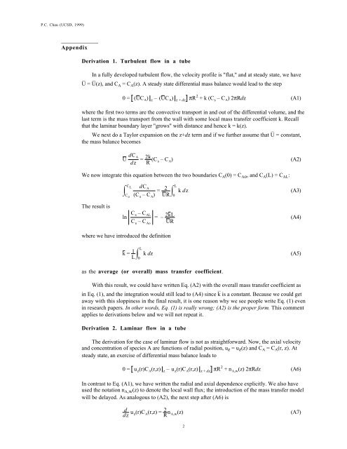
Derivation 1. Turbulent flow in a tube
In a fully developed turbulent flow, the velocity profile is "flat," and at steady state, we have
U – = U – (z), and C A = C A (z). A steady state differential mass balance would lead to the step
0= (UC A ) z –(UC A ) z+dz πR 2 +k(C s –C A )2πRdz (A1)
where the first two terms are the convective transport in and out of the differential volume, and the
last term is the mass transport from the wall with some local mass transfer coefficient k. Recall
that the laminar boundary layer "grows" with distance and hence k = k(z).
We next do a Taylor expansion on the z+dz term and if we further assume that U – = constant,
the mass balance becomes
U dC A
dz = 2k
R (C s –C A )
(A2)
We now integrate this equation between the two boundaries C A (0) = C Ao , and C A (L) = C AL :
C L dC A
= 2
(C s –C A ) UR
C o
0
L
k dz
(A3)
The result is
ln C s –C AL
C s –C Ao
=– 2kL
UR
(A4)
where we have introduced the definition
k = 1 L
0
L
k dz
(A5)
as the average (or overall) mass transfer coefficient.
With this result, we could have written Eq. (A2) with the overall mass transfer coefficient as
in Eq. (1), and the integration would still lead to (A4) since k – is a constant. Because we could get
away with this sloppiness in the final result, it is one reason why we see people write Eq. (1) even
in research papers. In other words, Eq. (1) is really wrong; (A2) is the proper form. This comment
applies to derivations below and we will not repeat it.
Derivation 2. Laminar flow in a tube
The derivation for the case of laminar flow is not as straightforward. Now, the axial velocity
and concentration of species A are functions of radial position, u z = u z (z) and C A = C A (r, z). At
steady state, an exercise of differential mass balance leads to
0= u z (r)C A (r,z) z –u z (r)C A (r,z) z+dz πR 2 +n A,w (z) 2πRdz (A6)
In contrast to Eq. (A1), we have written the radial and axial dependence explicitly. We also have
used the notation n A,w (z) to denote the local wall flux; the introduction of the mass transfer model
will be delayed. As analogous to (A2), the next step after (A6) is
d
dz u z(r)C A (r,z) = 2 R n A,w(z)
(A7)
2