Self-Avoiding Walk in Four Dimensions - Department of Mathematics
Self-Avoiding Walk in Four Dimensions - Department of Mathematics
Self-Avoiding Walk in Four Dimensions - Department of Mathematics

You also want an ePaper? Increase the reach of your titles
YUMPU automatically turns print PDFs into web optimized ePapers that Google loves.
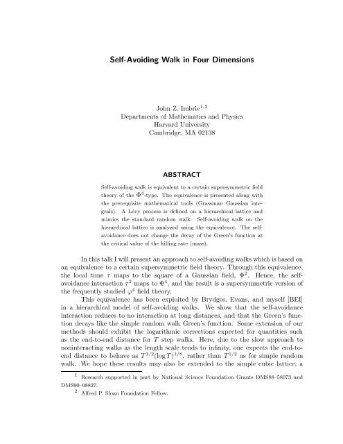
<strong>Self</strong>-<strong>Avoid<strong>in</strong>g</strong> <strong>Walk</strong> <strong>in</strong> <strong>Four</strong> <strong>Dimensions</strong><br />
John Z. Imbrie 1,2<br />
<strong>Department</strong>s <strong>of</strong> <strong>Mathematics</strong> and Physics<br />
Harvard University<br />
Cambridge, MA 02138<br />
ABSTRACT<br />
<strong>Self</strong>-avoid<strong>in</strong>g walk is equivalent to a certa<strong>in</strong> supersymmetric field<br />
theory <strong>of</strong> the Φ 4 -type. The equivalence is presented along with<br />
the prerequisite mathematical tools (Grassman Gaussian <strong>in</strong>tegrals).<br />
A Lévy process is def<strong>in</strong>ed on a hierarchical lattice and<br />
mimics the standard random walk.<br />
<strong>Self</strong>-avoid<strong>in</strong>g walk on the<br />
hierarchical lattice is analyzed us<strong>in</strong>g the equivalence.<br />
The selfavoidance<br />
does not change the decay <strong>of</strong> the Green’s function at<br />
the critical value <strong>of</strong> the kill<strong>in</strong>g rate (mass).<br />
In this talk I will present an approach to self-avoid<strong>in</strong>g walks which is based on<br />
an equivalence to a certa<strong>in</strong> supersymmetric field theory. Through this equivalence,<br />
the local time τ maps to the square <strong>of</strong> a Gaussian field, Φ 2 . Hence, the selfavoidance<br />
<strong>in</strong>teraction τ 2 maps to Φ 4 , and the result is a supersymmetric version <strong>of</strong><br />
the frequently studied ϕ 4 field theory.<br />
This equivalence has been exploited by Brydges, Evans, and myself [BEI]<br />
<strong>in</strong> a hierarchical model <strong>of</strong> self-avoid<strong>in</strong>g walks. We show that the self-avoidance<br />
<strong>in</strong>teraction reduces to no <strong>in</strong>teraction at long distances, and that the Green’s function<br />
decays like the simple random walk Green’s function. Some extension <strong>of</strong> our<br />
methods should exhibit the logarithmic corrections expected for quantities such<br />
as the end-to-end distance for T step walks. Here, due to the slow approach to<br />
non<strong>in</strong>teract<strong>in</strong>g walks as the length scale tends to <strong>in</strong>f<strong>in</strong>ity, one expects the end-toend<br />
distance to behave as T 1/2 (log T ) 1/8 , rather than T 1/2 as for simple random<br />
walk. We hope these results may also be extended to the simple cubic lattice, a<br />
1 Research supported <strong>in</strong> part by National Science Foundation Grants DMS88–58073 and<br />
DMS90–08827.<br />
2 Alfred P. Sloan Foundation Fellow.
longstand<strong>in</strong>g problem.<br />
The most familiar form <strong>of</strong> the self-avoid<strong>in</strong>g walk is obta<strong>in</strong>ed by enumerat<strong>in</strong>g<br />
all self-avoid<strong>in</strong>g walks <strong>of</strong> length T . Such a walk is described by a function ω :<br />
Z + → Z d <strong>in</strong> d dimensions, with ω(0) = 0, |ω(i) − ω(i + 1)| = 1 and ω(i) ≠ ω(j) for<br />
i ≠ j. One puts count<strong>in</strong>g measure on the set <strong>of</strong> T step self-avoid<strong>in</strong>g walks. Lett<strong>in</strong>g<br />
the associated expectation be denoted 〈·〉, one can analyze the asymptotics <strong>of</strong> the<br />
end-to-end distance:<br />
〈ω(T ) 2 〉 1/2 ∼ T ν .<br />
Here ν = ν(d) is one <strong>of</strong> the critical exponents <strong>of</strong> self-avoid<strong>in</strong>g walks. One expects<br />
ν = 1 2 for d > 4, thought this is proven only for d larger than some d 0 [S]. A weakly<br />
self-avoid<strong>in</strong>g walk is a bit easier to study, but should have the same exponents. In<br />
this case one does not assume ω(i) ≠ ω(j) for i ≠ j, and <strong>in</strong>stead weights each walk<br />
by a factor proportional to<br />
∏<br />
(1 − λδ(ω(i) − ω(j))) . (1)<br />
i 4, and nontrivial behavior (ν > 1 2<br />
) expected for d > 4. This<br />
should be signaled by the appearance <strong>of</strong> logarithms. Detailed predictions for the<br />
logarithms have been made by extend<strong>in</strong>g renormalization group calculations for n-<br />
vector φ 4 models to n = 0 [BLZ, De, Du]. The equivalence with the supersymmetric<br />
Φ 4 model can be thought <strong>of</strong> as a rigorous version <strong>of</strong> the n = 0 limit. At least it is<br />
the representation which appears most suited for rigorous analysis <strong>of</strong> self-avoid<strong>in</strong>g<br />
walks.<br />
We slightly change the underly<strong>in</strong>g random walk process by work<strong>in</strong>g <strong>in</strong> cont<strong>in</strong>uous<br />
time. This means that the unperturbed measure is def<strong>in</strong>ed by a system <strong>of</strong><br />
probabilities p(t, x), t ∈ R + , x ∈ Z d , satisfy<strong>in</strong>g<br />
∑<br />
p(t, x) = 1 ,<br />
x<br />
and the diffusion equation<br />
where ∆ is the lattice Laplacian.<br />
random walk <strong>in</strong> cont<strong>in</strong>uous time:<br />
p t = ∆p ,<br />
We can def<strong>in</strong>e a Green’s function for simple<br />
G 0x =<br />
∫ ∞<br />
0<br />
dt p(t, x) =<br />
∫ ∞<br />
0<br />
dt e t∆ (0, x)
= (−∆) −1 (0, x)<br />
= 1 N<br />
∫<br />
− 1 2<br />
φ 0 φ x e<br />
∑<br />
x<br />
(∇φ) 2 x<br />
∏<br />
dφ y . (2)<br />
y<br />
In the last l<strong>in</strong>e we have used the fact that the <strong>in</strong>verse <strong>of</strong> any operator can be<br />
obta<strong>in</strong>ed as the covariance <strong>of</strong> some Gaussian <strong>in</strong>tegral. In this case the operator is<br />
the Laplacian, lead<strong>in</strong>g to the (∇φ) 2 term <strong>in</strong> the Gaussian measure.<br />
Equation (2) expresses simple random walk as a path <strong>in</strong>tegral. Before attempt<strong>in</strong>g<br />
the same th<strong>in</strong>g for self-avoid<strong>in</strong>g walks, we need to replace the <strong>in</strong>teraction<br />
(1) with someth<strong>in</strong>g appropriate to the cont<strong>in</strong>uous time framework. We replace (1)<br />
with<br />
[ ∫ T ∫ ]<br />
T<br />
exp −λ ds dt δ(ω(s) − ω(t))<br />
0<br />
0<br />
= exp<br />
[<br />
−λ ∑ x<br />
∫ T<br />
0<br />
∫ ]<br />
T<br />
ds δ(ω(s) − x) dt δ(ω(t) − x)<br />
0<br />
= exp<br />
[<br />
−λ ∑ x<br />
τ 2 x<br />
]<br />
.<br />
Here<br />
τ x =<br />
∫ T<br />
0<br />
dt δ(ω(t) − x)<br />
is the time <strong>in</strong> [0, T ] spent at x, the “local time.” We can now def<strong>in</strong>e the Green’s<br />
function for self-avoid<strong>in</strong>g walk<br />
∫ (<br />
∞<br />
G SAW<br />
0x (s) = dT e<br />
〈exp<br />
sT −λ ∑ )<br />
〉<br />
τx<br />
2 δ(ω(T ) − x) , (3)<br />
0<br />
x<br />
where 〈·〉 is the expectation determ<strong>in</strong>ed by simple random walk, i.e., by the probabilities<br />
{p(t, x)}.<br />
Note the appearance <strong>of</strong> a Laplace transform variable s dual to T . This was<br />
suppressed <strong>in</strong> (2) because s = 0 was the critical value where G 0x exhibits power<br />
law decay. In (3) we need to adjust s to some nonzero value to compensate for the<br />
kill<strong>in</strong>g rate <strong>in</strong>duced by the self-avoidance <strong>in</strong>teraction. It is the critical value <strong>of</strong> s<br />
which is relevant for the long-time behavior <strong>of</strong> self-avoid<strong>in</strong>g walk. If one wishes to<br />
evaluate quantities such as the end-to-end distance for T step walks, one would have<br />
to <strong>in</strong>vert the Laplace transform. What is important then is the behavior <strong>of</strong> G 0x (s)
<strong>in</strong> the neighborhood <strong>of</strong> the critical value s = s c . We believe that the analysis lead<strong>in</strong>g<br />
to the asymptotics <strong>of</strong> the end-to-end distance can be done, but we will consider here<br />
only the asymptotics <strong>of</strong> G 0x (s c ).<br />
Let us now proceed to the field theory representation for G SAW<br />
0x (s). It was<br />
orig<strong>in</strong>ally derived by McKane [M] and Parisi-Sourlas [PS]. Let F (τ) be any function<br />
<strong>of</strong> local times τ = {τ x } (for the process <strong>in</strong> [0, T ]). We claim that<br />
∫ ∞<br />
0<br />
∫<br />
dT 〈F (τ)δ(ω(T ) − x)〉 =<br />
φ 0 φ x F (φ 2 − 1 2<br />
)e<br />
∑<br />
x<br />
(∇φ) 2 x<br />
∏<br />
dφ y . (4)<br />
y<br />
Note that tak<strong>in</strong>g F = 1, we recover (2). To obta<strong>in</strong> G SAW<br />
0x<br />
[<br />
]<br />
F = exp s ∑ τ x − λ ∑<br />
x<br />
x<br />
s<strong>in</strong>ce T = ∑ x τ x. Then on the right-hand side we obta<strong>in</strong><br />
[<br />
]<br />
F (φ 2 ) = exp s ∑ φ 2 x − λ ∑<br />
x<br />
x<br />
τ 2 x<br />
φ 4 x<br />
,<br />
we need only take<br />
,<br />
lead<strong>in</strong>g to a φ 4 field theory.<br />
To prove the claim, note that it is l<strong>in</strong>ear <strong>in</strong> F so it is sufficient to verify it<br />
for functions <strong>of</strong> the form exp[ ∑ x v xτ x ]. In this case we have<br />
〈 ( ) 〉 〈 ( ∑ ∫ )<br />
〉<br />
T<br />
exp v x τ x δ(ω(T ) − x) = exp v(ω(t)) dt δ(ω(T ) − x)<br />
x<br />
0<br />
= e T H (0, x) ,<br />
where H = ∆ + v. This is the Feynman-Kac formula. Therefore, apply<strong>in</strong>g steps as<br />
<strong>in</strong> (2), we obta<strong>in</strong><br />
∫ ∞<br />
0<br />
dT 〈F (τ)δ(ω(T ) − x)〉 =<br />
∫ ∞<br />
0<br />
dT e T H (0, x)<br />
= (−∆ − v) −1 (0, x)<br />
= 1 N ′ ∫<br />
= 1 N ′ ∫<br />
− 1 2<br />
φ 0 φ x e<br />
∑<br />
x<br />
φ 0 φ x F (φ 2 − 1 2<br />
)e<br />
(∇φ) 2 x − 1 2<br />
∑<br />
x<br />
∑<br />
x<br />
v x φ 2 x<br />
(∇φ) 2 x ∏<br />
y<br />
∏<br />
dφ y<br />
y<br />
dφ y . (5)
Here N ′ is the normalization for the v-dependent Gaussian measure exhibited on<br />
the third l<strong>in</strong>e. Note that except for this factor, the claim (4) is verified.<br />
Grassman Integrals. Unfortunately, <strong>in</strong> the present framework, the factor<br />
N ′ will not go away. To obta<strong>in</strong> a true statement, we have to generalize our notion<br />
<strong>of</strong> Gaussian <strong>in</strong>tegral to allow for Grassman variables as well as ord<strong>in</strong>ary variables.<br />
One can arrange for the two types <strong>of</strong> normalization factors to cancel, so that for an<br />
appropriate generalization <strong>of</strong> φ, N ′ = 1 and (4) holds. See [L], [BM] for some other<br />
applications.<br />
It is fairly straightforward to def<strong>in</strong>e the needed Grassman algebra and its<br />
associated <strong>in</strong>tegration theory (the Bérez<strong>in</strong> <strong>in</strong>tegral [B]). Let G be the algebra over<br />
the r<strong>in</strong>g <strong>of</strong> complex valued C ∞ functions on R 2n with a 2n-tuple { ¯ψ 1 , ψ 1 , . . . , ¯ψ n , ψ n }<br />
<strong>of</strong> generators satisfy<strong>in</strong>g the anticommutation relations:<br />
ψ # i ψ# j + ψ# j ψ# i<br />
= 0 i, j = 1, . . . , n, ψ # i<br />
= ψ i or ¯ψ i .<br />
The elements <strong>of</strong> G can be uniquely represented <strong>in</strong> the form<br />
g = ∑ α<br />
g (α) (φ)ψ α ,<br />
where α is a multi-<strong>in</strong>dex with 2n components (ᾱ 1 , α 1 , . . . , ᾱ n , α n ) which take values<br />
0 or 1, and where<br />
ψ α = ¯ψᾱ1 1 ψα 1<br />
1 · · · ¯ψᾱn n ψα n<br />
n .<br />
For each α, g (α) (φ) ≡ g (α) (φ, ¯φ) is a C ∞ function on R 2n , but we use complex conjugate<br />
variables ( ¯φ 1 , φ 1 , . . . , ¯φ n , φ n ) to denote a po<strong>in</strong>t <strong>in</strong> R 2n . The Bérez<strong>in</strong> <strong>in</strong>tegral<br />
is the map ∫ d α ψ : G → G which is l<strong>in</strong>ear over C ∞ (R 2n ) and satisfies<br />
∫<br />
d α ψ(ψ α ψ β ) = π −|α|/2 ψ β<br />
whenever ψ α ψ β ≠ 0. If α = (1, 1, . . . , 1), we write d α ψ = dψ. We may assemble all<br />
fields <strong>in</strong>to a s<strong>in</strong>gle vector Φ i = ( ¯φ i , φ i , ¯ψ i ψ i ). Then it is natural to def<strong>in</strong>e comb<strong>in</strong>ed<br />
Boson ( ¯φ, φ) and Fermion ( ¯ψ, ψ) <strong>in</strong>tegration by putt<strong>in</strong>g<br />
∫<br />
∫<br />
dΦg =<br />
∫<br />
dφ<br />
dψ g<br />
for any g ∈ G. Here dφ = d n (Re φ)d n (Im φ).<br />
With these def<strong>in</strong>itions it is not hard to verify that<br />
∫<br />
dψe −ψA ¯ψ = π −n det A
for any complex n × n matrix. In contrast,<br />
∫<br />
dφe −φA ¯φ = π −n (det A) −1 ,<br />
provided the real part A + Āt <strong>of</strong> A is positive def<strong>in</strong>ite. Thus, as desired, the<br />
normalizations cancel, and we def<strong>in</strong>e a comb<strong>in</strong>ed Fermion-Boson Gaussian measure<br />
dµ c (Φ) = dΦe −φA ¯φ−ψA ¯ψ ,<br />
where C = A −1 . It may be surpris<strong>in</strong>g, given the completely different <strong>in</strong>tegration<br />
theories, that this Gaussian measure is calculationally very similar to the standard<br />
Gaussian <strong>in</strong>tegral. For example,<br />
∫<br />
∫<br />
dµ c (Φ) ¯φ i φ j = dµ c (Φ) ¯ψ i ψ j = C ij ,<br />
and other moments can be evaluated us<strong>in</strong>g the usual Wick rules (but with m<strong>in</strong>us<br />
signs com<strong>in</strong>g from the anticommutation relations).<br />
In an ord<strong>in</strong>ary Gaussian <strong>in</strong>tegral where φ is an n-component vector, the<br />
normalization is (det A) −n/2 . S<strong>in</strong>ce this cancels <strong>in</strong> the comb<strong>in</strong>ed measure, one can<br />
th<strong>in</strong>k <strong>of</strong> the system as an n = 0 component vector, the two Fermionic components<br />
“cancel” the two Bosonic ones.<br />
Us<strong>in</strong>g the comb<strong>in</strong>ed Gaussian measure, we can now write down a corrected<br />
form <strong>of</strong> (5).<br />
Theorem 1. Let F ∈ C ∞ (R n + ) satisfy |F (τ)| ≤ const·exp(−b ∑ τ i ) for some b > 0.<br />
Then<br />
⎧ ⎫<br />
∫ ∞<br />
∫<br />
⎨ ¯ψ 0 ψ x ⎬<br />
dT 〈F (τ)δ(ω(T ) − x)〉 = dµ c (Φ)F (Φ 2 ) or<br />
0<br />
⎩ ⎭ ¯φ ,<br />
0 φ x<br />
where C = (−∆) −1 . More generally C is the <strong>in</strong>verse <strong>of</strong> the generator <strong>of</strong> any cont<strong>in</strong>uous<br />
time Markov cha<strong>in</strong> ω.<br />
Apply<strong>in</strong>g this theorem to self-avoid<strong>in</strong>g walk we obta<strong>in</strong><br />
∫<br />
[<br />
G SAW<br />
0x (s) = dµ c (Φ) ¯φ 0 φ x exp s ∑ Φ 2 x − λ ∑ ]<br />
(Φ 2 x) 2 . (6)<br />
x<br />
x<br />
The Hierarchical Model. In [BEI], a Lévy process (cont<strong>in</strong>uous time<br />
Markov cha<strong>in</strong>) is constructed on a hierarchical lattice G = ⊕ ∞<br />
j=0 Z n. The jump<strong>in</strong>g<br />
rates are chosen <strong>in</strong> such a way that the Green’s function mimics the <strong>in</strong>verse<br />
Laplacian. Def<strong>in</strong>e the length <strong>of</strong> any po<strong>in</strong>t x ∈ G:<br />
{ 0, x = 0,<br />
|x| H =<br />
L p , p = <strong>in</strong>f {k : x ∈ G k },
where G k = ⊕ k<br />
j=0 Z n. Tak<strong>in</strong>g n = L p , we can th<strong>in</strong>k <strong>of</strong> G k as a block <strong>of</strong> L dk po<strong>in</strong>ts<br />
such as would arise <strong>in</strong> a renormalization group scheme on the simple cubic lattice.<br />
Then, for most x, y, |x − y| H is comparable to the Euclidean distance |x − y|.<br />
Endow<strong>in</strong>g the hierarchical lattice with a group structure permits the use<br />
<strong>of</strong> the <strong>Four</strong>ier transform to compute the Green’s function. Specifically, <strong>in</strong> <strong>Four</strong>ier<br />
transform variables, the Green’s functions is the <strong>in</strong>verse <strong>of</strong> the <strong>in</strong>f<strong>in</strong>itesimal generator<br />
<strong>of</strong> the process. The follow<strong>in</strong>g result is obta<strong>in</strong>ed <strong>in</strong> [BEI].<br />
Theorem 2. Consider the Lévy process on G <strong>in</strong> which jumps from x to y have<br />
probability proportional to |x − y| −(d+2)<br />
H<br />
. The jump<strong>in</strong>g rate may be chosen so that<br />
the Green’s function is<br />
{<br />
−(d−2)<br />
G xy = |x − y|<br />
H<br />
, x ≠ y<br />
(1 − L −d )/(1 − L −2 (7)<br />
), x = y.<br />
The Renormalization Group. Let us apply the field theory representation<br />
(6) to the hierarchical model. The covariance <strong>of</strong> the Gaussian measure is given by<br />
(7). It can be split as<br />
G = G ′ + Γ<br />
where<br />
G ′ (x) = L −2 G(x/L) .<br />
Here division by L corresponds to a shift <strong>in</strong> G = ⊕ Z n . The “fluctuation covariance”<br />
Γ vanishes if |x − y| H > L. A renormalization group transformation can be def<strong>in</strong>ed<br />
by writ<strong>in</strong>g ∫<br />
∫<br />
dµ G (Φ)F (Φ) = dµ G ′(Φ ′ )dµ Γ (δ)F (Φ ′ + ζ)<br />
= dµ G (Φ)(T F )(Φ) .<br />
In the second step, we have rescaled Φ ′ and replaced blocks with po<strong>in</strong>ts, us<strong>in</strong>g the<br />
constancy <strong>of</strong> G ′ on blocks.
In the case at hand, F = ∏ x f(Φ x). S<strong>in</strong>ce Γ does not couple different L d -<br />
blocks, T F is also a product. Hence, T can be viewed as a transformation on<br />
functions f. Except for the presence <strong>of</strong> Fermionic variables, this transformation is<br />
similar to ones studied by [BlS], [GK].<br />
The follow<strong>in</strong>g result on the action <strong>of</strong> the renormalization group on the hierarchical<br />
self-avoid<strong>in</strong>g walk is proven <strong>in</strong> [BEI]. The formulation uses wick ordered<br />
powers <strong>of</strong> Φ, which are def<strong>in</strong>ed as<br />
:P (Φ): = exp(−∆)P (Φ) ,<br />
∆ ≡ ∑ { ∂<br />
G(x − y)<br />
∂ψ(x)<br />
x,y<br />
∂<br />
∂ ¯ψ(y) +<br />
∂<br />
∂φ(x)<br />
}<br />
∂<br />
∂ ¯φ(y)<br />
Theorem 3. Let d = 4. Assume µ 2 , η are O(λ 2 ), with λ small. Suppose<br />
g(Φ) = e −λ:(Φ2 ) 2 :+µ 2 :Φ 2: (1 + η:(Φ 2 ) 3 :) + r(Φ) ,<br />
with rema<strong>in</strong>der r(Φ) depend<strong>in</strong>g only on Φ 2 , and satisfy<strong>in</strong>g<br />
∑<br />
α<br />
sup<br />
φ<br />
∣<br />
∣<br />
∂ α r(Φ)<br />
e λ1/2 |φ| ∣∣∣ 2 ≤ O(λ) .<br />
α!<br />
Then T g satisfies the same properties, except that λ, µ 2 , η are replaced with primed<br />
parameters obey<strong>in</strong>g<br />
λ ′ = λ − βλ 2 + O(λ 3 )<br />
µ ′2 = L 2 µ 2 + γλ 2 + O(λ 3 ) .<br />
Theorem 3 shows that the model is asymptotically free. This means that for<br />
a certa<strong>in</strong> choice <strong>of</strong> µ 2 = µ 2 c(λ), the parameter λ is driven to zero under successive<br />
applications <strong>of</strong> the transformation T .<br />
Further analysis <strong>of</strong> the “observables” φ 0 ¯φx <strong>in</strong> (6) leads to the follow<strong>in</strong>g<br />
asymptotic statement for the self-avoid<strong>in</strong>g walk Green’s function (at the critical<br />
µ 2 c (λ)): G SAW<br />
xy (µ 2 c(λ)) = (1 + O(λ))G(x − y)(1 + ɛ(x − y))<br />
.<br />
|ɛ(x)| ≤ λ(1 + λ log |x|) −1 .<br />
Thus the decay <strong>of</strong> the Green’s function for self-avoid<strong>in</strong>g walk is the same as that <strong>of</strong><br />
the Green’s function <strong>of</strong> the hierarchical Lévy process.
References.<br />
[B] Bérez<strong>in</strong>, F. A.: The Method <strong>of</strong> Second Quantization. Academic Press, New<br />
York (1966).<br />
[BlS] Bleher, P. M., and S<strong>in</strong>ai, Ya. G.: Investigation <strong>of</strong> the Critical Po<strong>in</strong>t <strong>in</strong> Models<br />
<strong>of</strong> the Type <strong>of</strong> Dyson’s Hierarchical Models. Commun. Math. Phys. 33,<br />
23–42 (1973).<br />
[BLZ] Bérez<strong>in</strong>, E., Le Guillou, J. C., and Z<strong>in</strong>n-Just<strong>in</strong>, J.: Phase Transitions and<br />
Critical Phenomena, Vol. VI. Domb, C. and Green, M. S. (eds.): Academic<br />
Press, New York (1976).<br />
[BEI] Brydges, D., Evans, S. N., and Imbrie, J. Z.: <strong>Self</strong>-<strong>Avoid<strong>in</strong>g</strong> <strong>Walk</strong> on a Hierarchical<br />
Lattice <strong>in</strong> <strong>Four</strong> <strong>Dimensions</strong>. Ann. Prob., to appear.<br />
[BM] Brydges, D. C., and Munoz-Maya, I.: An Application <strong>of</strong> Berez<strong>in</strong> Integration<br />
to Large Deviations. University <strong>of</strong> Virg<strong>in</strong>ia prepr<strong>in</strong>t, 1989.<br />
[BS] Brydges, D., and Spencer, T.: <strong>Self</strong>-<strong>Avoid<strong>in</strong>g</strong> <strong>Walk</strong> <strong>in</strong> 5 or More <strong>Dimensions</strong>.<br />
Commun. Math. Phys. 97, 125–148 (1985).<br />
[De] De Gennes, P. G.: Exponents for the Excluded Volume Problem as Derived<br />
by the Wilson Method: Physics Lett. 38A, 339–340 (1972).<br />
[Du] Duplantier, B.: Polymer Cha<strong>in</strong>s <strong>in</strong> <strong>Four</strong> <strong>Dimensions</strong>. Nucl. Phys. B275,<br />
319–355 (1986).<br />
[GK] Gawedzki, K., and Kupia<strong>in</strong>en, A.: Asymptotic Freedom Beyond Perturbation<br />
Theory. In: Critical Phenomena, Random Systems, Gauge Theories,<br />
Les Houches 1984. Osterwalder, K., and Stora, R. (eds.): North Holland,<br />
Amsterdam (1986).<br />
Gawedzki, K., and Kupia<strong>in</strong>en, A.: Triviality <strong>of</strong> ϕ 4 4 and All That <strong>in</strong> a Hierarchical<br />
Model Approximation. J. Stat. Phys. 29, 683–698 (1982).<br />
[L] Lutt<strong>in</strong>ger, J. M.: The Asymptotic Evaluation <strong>of</strong> a Class <strong>of</strong> Path Integrals II.<br />
Journal <strong>of</strong> Mathematical Physics 24, 2070–2073 (1983).<br />
[M] McKane, A. J.: Reformulation <strong>of</strong> n → 0 Models Us<strong>in</strong>g Anticommut<strong>in</strong>g Scalar<br />
Fields. Phys. Lett. 76A, 22–24 (1980).<br />
[PS] Parisi, G., and Sourlas, N.: <strong>Self</strong>-<strong>Avoid<strong>in</strong>g</strong> <strong>Walk</strong> and Supersymmetry. J.<br />
Phys. Lett. 41, L403–L406 (1980).<br />
Parisi, G., and Sourlas, N.: Random Magnetic Fields, Supersymmetry and<br />
Negative <strong>Dimensions</strong>. Phys. Lett. 43, 744–745 (1979).<br />
[S] Slade, G.: The Diffusion <strong>of</strong> <strong>Self</strong>-<strong>Avoid<strong>in</strong>g</strong> Random <strong>Walk</strong> <strong>in</strong> High <strong>Dimensions</strong>.<br />
Commun. Math. Phys. 110, 661–683 (1987).