An evaluation of lattice Boltzmann schemes for por... - ResearchGate

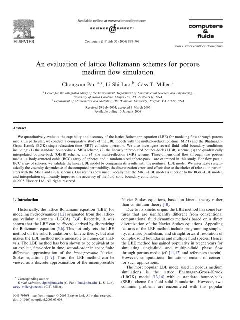
Computers & Fluids 35 (2006) 898–909 

www.elsevier.com/locate/compfluid 

An evaluation of lattice Boltzmann schemes for porous 

medium flow simulation 

Chongxun Pan a, *, Li-Shi Luo b , Cass T. Miller a 

a Center for the Integrated Study of the Environment, Department of Environmental Sciences and Engineering, 

University of North Carolina, Chapel Hill, NC 27599-7431, USA 

b Department of Mathematics and Statistics, Old Dominion University, Norfolk, VA 23529, USA 

Received 29 July 2004; accepted 8 March 2005 

Available online 10 January 2006 

Abstract 

We quantitatively evaluate the capability and accuracy of the lattice Boltzmann equation (LBE) for modeling flow through porous 

media. In particular, we conduct a comparative study of the LBE models with the multiple-relaxation-time (MRT) and the Bhatnagar– 

Gross–Krook (BGK) single-relaxation-time (SRT) collision operators. We also investigate several fluid–solid boundary conditions 

including: (1) the standard bounce-back (SBB) scheme, (2) the linearly interpolated bounce-back (LIBB) scheme, (3) the quadratically 

interpolated bounce-back (QIBB) scheme, and (4) the multi-reflection (MR) scheme. Three-dimensional flow through two porous 

media—a body-centered cubic (BCC) array of spheres and a random-sized sphere-pack—are examined in this study. For flow past a 

BCC array of spheres, we validate the linear LBE model by comparing its results with the nonlinear LBE model. We investigate systematically 

the viscosity-dependence of the computed permeability, the discretization error, and effects due to the choice of relaxation parameters 

with the MRT and BGK schemes. Our results show unequivocally that the MRT–LBE model is superior to the BGK–LBE model, 

and interpolation significantly improves the accuracy of the fluid–solid boundary conditions. 

Ó 2005 Elsevier Ltd. All rights reserved. 

1. Introduction 

Historically, the lattice Boltzmann equation (LBE) for 

modeling hydrodynamics [1,2] originated from the latticegas 

cellular automata (LGCA) [3,4]. Recently, it was 

shown that the LBE can be directly derived by discretizing 

the Boltzmann equation [5,6]. This not only sets the LBE 

method on the solid foundation of kinetic theory, but also 

makes the LBE method more amenable to numerical analysis. 

The LBE method has been shown to be equivalent to 

an explicit, first-order in time, second-order in space finite 

difference approximation of the incompressible Navier– 

Stokes equations [7–9]. Thus, the LBE method can be 

viewed as a discrete approximation of the incompressible 

* Corresponding author. 

E-mail addresses: dpan@unc.edu (C. Pan), lluo@odu.edu (L.-S. Luo), 

casey_miller@unc.edu (C.T. Miller). 

Navier–Stokes equations, based on kinetic theory rather 

than continuum theory [10]. 

Due to its kinetic origin, the LBE method has some features 

that are significantly different from conventional 

computational fluid dynamics methods based on a direct 

discretization of the Navier–Stokes equations. Appealing 

features of the LBE method include programming simplicity, 

intrinsic parallelism, and straightforward resolution of 

complex solid boundaries and multiple fluid species. Hence, 

the LBE method has gained popularity in recent years for 

simulating single-fluid and multiple-fluid phase flow 

through porous media (cf. [11,12] and references therein). 

However, computational limitations remain of concern 

for such applications. 

The most popular LBE model used in porous medium 

simulations is the lattice Bhatnagar–Gross–Krook 

(LBGK) model [13,14] with a standard bounce-back 

(SBB) scheme for fluid–solid boundaries. However, two 

common problems are encountered with this popular 

0045-7930/$ - see front matter Ó 2005 Elsevier Ltd. All rights reserved. 

doi:10.1016/j.compfluid.2005.03.008

C. Pan et al. / Computers & Fluids 35 (2006) 898–909 899 

method. First, the LBGK model, in which the collision 

operator is approximated by a single-relaxation-time 

(SRT) approximation, has some defects such as numerical 

instability and viscosity dependence of boundary locations, 

especially in under-relaxed situations [15]. The viscosity 

dependent boundary conditions pose a severe problem 

for simulating flow through porous media because the permeability 

becomes viscosity dependent, while it should be a 

characteristic of the physical properties of porous medium 

alone. The problem of the viscosity-dependence of the 

boundary conditions is clearly illustrated by Fig. 1, in 

which the computed permeability for a typical porous medium 

GB1b (cf. Section 5) varies significantly as the viscosity 

changes in the LBGK model. The deficiencies inherent in 

the LBGK model can be significantly reduced by using a 

multiple-relaxation-time (MRT) approach [16–22], which 

separates the relaxation times for different kinetic modes 

and allows tuning to improve numerical stability and 

accuracy. 

Second, in the LBE simulations of flow through a porous 

medium, curved fluid–solid interfaces are usually 

approximated using a zig-zag approach so that the SBB 

boundary conditions can be directly applied, which reverse 

the momentum of fluid particles colliding with a solid 

boundary by mimicking the particle–solid interaction for 

no-slip boundary conditions. The SBB boundary conditions 

are easy to implement; they do, however, introduce 

errors in boundary locations, especially when the resolution 

is coarse, and using fine enough uniform discretization 

of pore geometries to adequately resolve the flow with zigzag 

approximation is often ineffective and unrealistic computationally. 

Recently, several schemes have been 

advanced to more accurately represent such boundaries 

using spatial interpolations [12,22,23]. These methods can 

be incorporated separately into LBE model to further 

improve accuracy and to speed up convergence. However 

to the best of our knowledge, no systematic quantitative 

comparison of the numerical accuracy and convergence 

Normalized permeability 

2 

1.5 

1 

0.5 

1/30 0.1 1/6 1/3 

Viscosity 

Fig. 1. The viscosity dependence of the computed permeability using the 

LBGK model. The result is obtained for flow through a sphere-pack 

medium. 

rate of these methods has been reported in the literature 

for complex porous medium systems. 

The overall goal of the present work is to examine the 

accuracy of LBE models for the solution of flow through 

porous medium systems. The specific objectives of this 

work are: (1) to implement a standard LBGK and an 

MRT–LBE model with a number of fluid–solid boundary 

schemes; (2) to compare the numerical accuracy of available 

LBE schemes for model problems quantitatively and 

systematically; and (3) to investigate the discretization level 

necessary to achieve resolution-independent results for single-phase 

flow in porous media using various boundary 

schemes. 

The remaining parts of this paper are organized as follows. 

Section 2 describes briefly the three-dimensional 

MRT–LBE model with 19 velocities (D3Q19 model) used 

in this paper. Section 3 discusses the set of fluid–solid 

boundary conditions to be compared in the work, including 

the standard bounce-back (SBB) scheme, the linearly 

interpolated bounce-back (LIBB) scheme, the quadratically 

interpolated bounce-back (QIBB) scheme, and the multireflection 

(MR) scheme. Sections 4 and 5 present the 

numerical results for flow through a periodic body-centered 

cubic (BCC) array of spheres of equal radius and 

the results for flow through a random-sized sphere-pack 

porous medium, respectively. Finally, Section 6 concludes 

the paper. 

2. Multiple-relaxation-time LBE model 

There are three components in any LBE model. The first 

component is a discrete phase space consisting of a regular 

lattice space d x Z d with a lattice constant d x in d dimensions 

together with a finite set of highly symmetric discrete velocities 

{e i ji = 0,1, ...,N} connecting each lattice node 

x k 2 d x Z d to its neighbors, and the corresponding set of 

velocity distribution functions {f i ji =0,1,...,N} defined 

on each node of the lattice. The second component is a collision 

matrix S and (N + 1) equilibrium distribution functions 

ff ðeqÞ 

i j i ¼ 0; 1; ...; Ng. The equilibrium distribution 

functions are functions of the local conserved quantities 

and are a crucial component of the LBE method, which 

can be related to kinetic theory. The third component is 

an evolution equation in discrete time t n 2 d t N 0 : 

fðx k þ ed t ; t n þ d t Þ fðx k ; t n Þ 

 

¼ S f ðeqÞ ðx k ; t n Þ 

 

fðx k ; t n Þ þ F; ð1Þ 

or equivalently 

fðx k þ ed t ; t n þ d t Þ 

fðx k ; t n Þ 

¼ M 1 b S½m ðeqÞ ðx k ; t n Þ mðx k ; t n ÞŠ þ F; ð2Þ 

where the bold-face symbols, f, m, m (eq) , and F are B- 

dimensional (column) vectors (B = N +1orN for models 

with or without zero velocity, respectively), i.e.,

900 C. Pan et al. / Computers & Fluids 35 (2006) 898–909 

fðx k þ ed t ; t n þ d t Þ 

:¼ ðf 0 ðx k ; t n þ d t Þ; ...; f N ðx k þ e N d t ; t n þ d t ÞÞ T ; 

fðx k ; t n Þ :¼ ðf 0 ðx k ; t n Þ; f 1 ðx k ; t n Þ; ...; f N ðx k ; t n ÞÞ T ; 

mðx k ; t n Þ :¼ ðm 0 ðx k ; t n Þ; m 1 ðx k ; t n Þ; ...; m N ðx k ; t n ÞÞ T ; 

F :¼ ðF 0 ; F 1 ; ...; F N Þ T . 

Here superscript T denotes the transpose operator, and F 

represents the external forcing, of which the components are: 

e i a 

F i ¼ 3w i q 0 ; ð3Þ 

c 2 

where c :¼ d x /d t , q 0 is the (constant) mean density in the 

system (usually set to 1), a is the acceleration due to external 

forces, and the weight coefficients for the D3Q19 model 

are usually chosen as w 0 =1/3,w i = 1/18 for i = 1–6, and 

w i = 1/36 for i = 7–18. In lattice units, the time step d t is 

set equal to 1, as is the lattice spacing (d x = d t = 1). 

The relaxation matrix b S ¼ M S M 1 is a B · B diagonal 

matrix. The transformation matrix M relates the distribution 

functions represented by f 2 V ¼ R B to their 

moments represented by m 2 M ¼ R B , as in the following: 

m ¼ M f; f ¼ M 1 m. ð4Þ 

The transformation matrix M is constructed from the 

monomials of the discrete velocity components 

e m ia en jb el kc 

(a,b and c 2 {x,y,z}) via the Gram–Schmidt 

orthogonalization procedure [16,19–21]. The row vectors 

of M are mutually orthogonal, i.e., M M T is a diagonal 

matrix, but not normalized so all the matrix elements of 

M are integers [16,19–21]. For the 19-velocity model in 

three dimensions, i.e., the D3Q19 model (here DdQq 

denotes the model with q velocities in d dimensions), the 

matrix M is given in [20,24]. 

For the D3Q19 model, the 19 moments are: 

m :¼ ðq; e; e; j x ; q x ; j y ; q y ; j z ; q z ; 3p xx ; 3p xx ; p ww ; 

p ww ; p xy ; p yz ; p xz ; m x ; m y ; m z Þ T 

¼ðm 0 ; m 1 ; ...; m 18 Þ T ; 

among which, only the density q ¼ P i f i and momentum 

j :¼ ðj x ; j y ; j z Þ¼ P i f ie i are conserved quantities for athermal 

fluids, and the rest are non-conserved quantities [20]. 

The equilibria m (eq) (q,j) for the non-conserved moments 

are [20]: 

e ðeqÞ ¼ 11q þ 19 j j ¼ 11q þ 19 ðj 2 x 

q 0 q þ j2 y þ j2 z Þ; ð5aÞ 

0 

e ðeqÞ 11 

¼ 3q j j; 

ð5bÞ 

2q 0 

q ðeqÞ 

x 

¼ 2 3 j x; q ðeqÞ 

y 

¼ 2 3 j y; q ðeqÞ 

z 

¼ 2 3 j z; ð5cÞ 

p ðeqÞ 

xx 

¼ 1 h 

i 

2j 2 x 

ðj 2 y 

3q þ j2 z Þ ; p ðeqÞ 

ww ¼ 1 h i 

j 2 y 

j 2 z 

; ð5dÞ 

0 q 0 

p ðeqÞ 

xy 

¼ 1 j 

q x j y ; p ðeqÞ 

yz 

¼ 1 j 

0 q y j z ; p ðeqÞ 

xz 

¼ 1 j 

0 q x j z ; ð5eÞ 

0 

p ðeqÞ 

xx 

¼ 1 2 pðeqÞ xx 

; p ðeqÞ 

ww ¼ 1 2 pðeqÞ ww ; 

m ðeqÞ 

x 

¼ m ðeqÞ 

y 

¼ m ðeqÞ 

z 

¼ 0. ð5fÞ 

Corresponding the particular order of moments used here, 

the diagonal relaxation matrix b S is given by 

bS ¼ diagð0;s 1 ;s 2 ;0;s 4 ;0;s 4 ;0;s 4 ;s 9 ;s 10 ;s 9 ;s 10 ;s 13 ;s 13 ;s 13 ;s 16 ;s 16 ;s 16 Þ 

¼ diagð0;s e ;s e ;0;s q ;0;s q ;0;s q ;s m ;s p ;s m ;s p ;s m ;s m ;s m ;s m ;s m ;s m Þ. 

ð6Þ 

p 

The speed of sound of the model is c s ¼ 1= 

ffiffiffi 

3 and the 

viscosity is 

m ¼ 1 

1 1 

. ð7Þ 

3 s m 2 

With the above equilibria of Eqs. (5a), if all of the relaxation 

rates, {s i ji =0,...,18}, are set to be a single value 1/s, 

i.e., S ¼ s 1 I, where I is B · B identity matrix, then the 

model is equivalent to an LBGK model with the following 

equilibria [5]: 

 

f ðeqÞ 

i ðq; uÞ ¼w i q þ q 0 3e i u þ 9 2 ðe i uÞ 2 3 

2 u u 

 

 

. ð8Þ 

where the fluid velocity u :¼ j/q 0 . When external forcing F 

is considered in the LBE simulations, j 0 = j + q 0 ad t /2 (or 

u 0 = u + ad t /2), instead of j (or u), is used as the measured 

velocity field for output, and in the calculation of nonlinear 

velocity terms of the equilibria of Eq. (5a) for the moments 

(or equilibria of Eq. (8) for the distributions). The reason 

of replacing j by j 0 for output and in nonlinear term calculations 

is to account for the momentum change due to F 

and to satisfy the mass conservation equation up to the 

second-order in the Chapman–Enskog analysis [22,21]. 

For more detailed discussions of the discrete lattice effects 

on the external forcing term and MRT–LBE method in 

general, we refer readers to the literature [16–22]. 

When simulating flow through porous media, we are 

often interested in Stokes flow, for which Darcy’s law 

holds. The Stokes flow can be simulated by the linear 

LBE scheme, in which all the nonlinear velocity terms are 

omitted in the equilibria given by Eq. (5a) for the moments, 

or equivalently in the the equilibria of Eq. (8) for the distribution 

functions, i.e., 

e ðeqÞ ¼ 11q; e ðeqÞ ¼ 3q; ð9aÞ 

q ðeqÞ 

x 

¼ 2 3 j x; q ðeqÞ 

y 

¼ 2 3 j y; q ðeqÞ 

z 

¼ 2 3 j z; ð9bÞ 

p ðeqÞ 

xx 

p ðeqÞ 

xx 

¼ p ðeqÞ 

ww 

¼ p ðeqÞ 

ww 

¼ pðeqÞ xy 

¼ p ðeqÞ 

yz 

¼ 0; mðeqÞ 

x 

¼ p ðeqÞ 

xz 

¼ 0; ð9cÞ 

¼ m ðeqÞ 

y 

¼ m ðeqÞ 

z 

¼ 0. ð9dÞ 

With the above equilibria, the resulting momentum equation 

is the Stokes equation without the nonlinear advection 

term u $u. Note that Darcy’s law is only valid for the flow 

in the limit of zero Reynolds number [25], i.e., the Stokes 

flow. We will validate the linear LBE scheme in simulations 

of flow through a simple porous geometry.


3. Solid boundary conditions 

The LBE method deals with the single particle distribution 

function f in phase space C :¼ (x,n), as opposed to the 

hydrodynamic variables, such as fluid density q, flow 

velocity u, and temperature T, in physical space x. Consequently, 

the boundary conditions in the LBE method are 

also expressed in terms of the distribution function f rather 

than the flow variables commonly controlled in conventional 

computational fluid dynamics methods. In the 

LBE method, the objective is to construct the unknown 

incoming distribution functions based on the known 

outgoing distribution functions at the boundary nodes so 

that the physical boundary conditions of interest are 

satisfied. 

The lattice Boltzmann scheme consists of two steps, i.e., 

collision : ~ f i ðx k ; t n Þ f i ðx k ; t n Þ¼X i ; ð10aÞ 

streaming : f i ðx k þ e i d t ; t n þ d t Þ¼ ~ f i ðx k ; t n Þ; ð10bÞ 

and x , i.e., q :¼ jx x j/jx x j = 1/2, the incoming 

where X i denotes the collision operator, and f ~ i and f i denote 

the post- and pre-collision states of the particle distribution 

Fig. 2. Illustration of the interpolated boundary conditions in one 

functions, respectively. During the streaming step, dimension. Symbols , d, s and h denote interior fluid node, boundary 

fluid node, the off-lattice location involved in interpolations, and solid 

the no-slip velocity boundary conditions at the fluid–solid 

node, respectively. (a) the perfect bounce-back situation, q = 1/2; (b) 

interface are usually approximated using the standard interpolation before the bounce-back collision, q < 1/2; and (c) interpolation 

after the bounce-back collision, q > 1/2. 

bounce-back (SBB) boundary conditions, which mimic 

the phenomenon that a particle reflects its momentum 

when colliding with a solid surface. 

It is important to stress that the SBB boundary 

condition does not always place the wall at the one-half 

boundary location x W is situated half-way between x A (LIBB) formulae for f L ðx A ; t nþ1 Þ¼ f ~ R ðx C ; t n Þ are: 

grid spacing beyond the last fluid node. In the LBGK 

model, the actual position of the boundary is viscosity 

dependent when the SBB is applied. This can be easily seen 

from the analytic solutions for the Poiseuille flow [15], 

B A W A B 

distribution function is simply equal to the corresponding 

outgoing one with the opposite momentum, hence the 

name ‘‘bounce-back’’ boundary conditions. 

Intuitively in the perfect bounce-back situation, in a 

especially in under-relaxed situations, i.e., when s > 1. This complete streaming-collision cycle the particle travels 

problem can be solved with the MRT–LBE model when 

using the linear LBE scheme, by combining the bounceback 

rule with a carefully constructed collision operator. 

Because the boundary location depends on a polynomial 

of relaxation rates {s i } [17,22], one can choose the relaxation 

rate s q for the ‘‘energy flux’’ mode q :¼ (q x ,q y ,q z )as 

the following: 

half-way between two nodes x A and x B , collides with the 

wall at x W , and reverses its momentum (the collision process 

is assumed not to consume any time), then travels back 

to x A , as illustrated by Fig. 2(a). When q < 1/2, the particle 

at x A would end up at x C after the streaming-collision 

cycle, as illustrated by the thin arrow in Fig. 2(b). However, 

if the particle starts from x C , then it will end up at x A after 

the streaming-collision cycle, as illustrated by the thick 

s q ¼ 8 ð2 s mÞ 

ð8 s m Þ ; ð11Þ arrow in Fig. 2(b). This can be accomplished if we can construct 

the distribution function at x C by using an interpolation 

before the streaming-collision process with the wall 

such that the position where u = 0 is fixed at exactly one 

half lattice spacing beyond the last fluid node for Poiseuille 

flow when the solid walls are parallel to the underlying 

lattice lines [17,18,22,23]. 

takes place. Similarly, when q > 1/2, the incoming distribution 

function can be constructed by using the outgoing one 

located at x C after the streaming-collision interaction with 

the wall takes place, as illustrated by the thick arrow in 

Fig. 2(c), and the distribution function values at nearby 

3.1. Interpolated bounce-back schemes 

nodes x D and x E . 

For stability considerations, we limit ourselves to interpolations, 

Fig. 2 illustrates the typical scenario in bounce-back 

boundary conditions in a one-dimensional setting. If the including linear and quadratic interpolations 

proposed in [23,26]. The linear interpolation bounce-back


f L ðx A ;t nþ1 Þ 

8 

< ð1 2qÞ f ~ R ðx D ;t n Þþ2q f ~ R ðx A ;t n Þ; q < 1=2; 

¼ 

f L ðx D ;t nþ1 Þþ 1 f ð12aÞ 

: 

2q Lðx C ;t nþ1 Þ; q P 1=2; 

1 

1 

2q 

8 

< ð1 2qÞf R ðx A ;t nþ1 Þþ2q f ~ R ðx A ;t n Þ; q < 1=2; 

¼ 

: 

 

~f 

L ðx A ;t n Þþ 1 f ~ 2q R ðx A ;t n Þ; q P 1=2. 

1 

1 

2q 

ð12bÞ 

In the above formulae, subscripts L and R indicate leftbound 

or right-bound directions, respectively, as depicted 

in Fig. 2. The interpolation formulae involve either the 

post-collision information at time t n or or pre-collision 

information at time t n+1 :¼ t n + d t . Hence, Eq. (12b) indicates 

that the LIBB requires only local information to perform 

interpolation. Similarly, the quadratic interpolation 

bounce-back (QIBB) formulae are: 

f L ðx A ;t nþ1 Þ 

8 

qð1 þ 2qÞ f ~ R ðx A ;t n Þþð1 

4q 2 Þ ~ f R ðx D ;t n Þ 

>< qð1 2qÞ f ~ R ðx E ;t n Þ; q < 1=2; 

¼ 

2q 1 

f 

q L ðx D ;t nþ1 Þþ 1 f qð2qþ1Þ Lðx C ;t nþ1 Þ 

>: 

þ ð1 2qÞ f ð1þ2qÞ Lðx E ;t nþ1 Þ; q P 1=2; 

8 

qð1 þ 2qÞ f ~ R ðx A ;t n Þþð1 4q 2 Þf R ðx A ;t nþ1 Þ 

>< qð1 2qÞf R ðx D ;t nþ1 Þ; q < 1=2; 

¼ 

2q 1 ~f 

q L ðx A ;t n Þþ 1 f ~ qð2qþ1Þ R ðx A ;t n Þ 

>: 

þ ð1 2qÞ f ~ ð1þ2qÞ L ðx D ;t n Þ; q P 1=2. 

ð13aÞ 

ð13bÞ 

Note that both linear and quadratic interpolations are upwind 

with respect to the particle velocity (e 1 in this case) 

when q < 1/2 and downwind when q > 1/2, and they reduce 

to the SBB boundary conditions when q = 1/2. 

3.2. Multi-reflection boundary conditions 

The multi-reflection (MR) boundary conditions [22] for 

solving the moving solid boundary problems, on the other 

hand, utilize a more general closure relation that determines 

the unknown distributions from five neighboring 

values. The closure relation is theoretically obtained from 

the Chapman–Enskog expansion at the boundary nodes. 

The MR closure relation is accurate up to third-order in 

the Chapman–Enskog expansion by considering a correction 

term E f ð2Þ 

i : 

f L ðx A ;t nþ1 Þ¼k 1 f L ðx C ;t nþ1 Þþk 2 f R ðx A ;t nþ1 Þþk 3 f R ðx D ;t nþ1 Þ 

þ k 4 f L ðx D ;t nþ1 Þþk 5 f L ðx E ;t nþ1 ÞþE L ðx A ;t n Þ 

ð14aÞ 

¼ k 1 f ~ R ðx A ;t n Þþk 2 f R ðx A ;t nþ1 Þþk 3 f R ðx D ;t nþ1 Þ 

þ k 4 f ~ L ðx A ;t n Þþk 5 f ~ L ðx D ;t n Þþ k 6 

m f ð2Þ 

L 

ðx A;t n Þ 

ð14bÞ 

where m is the viscosity given by Eq. (7). The coefficients k i , 

i 2 {1,2,...,6} are functions of q and are chosen as follows 

when the relation between the relaxation parameters of 

Eq. (11) is used (see detailed formulation in [22]): 

k 1 ¼ 1; k 2 ¼ k 4 ¼ ð1 2q 2q2 Þ 

ð1 þ qÞ 2 ; 

k 3 ¼ k 5 ¼ 

q2 

ð1 þ qÞ 2 ; 

k 6 ¼ 

1 

4ð1 þ qÞ 2 . 

ð15Þ 

The third-order nonequilibrium terms f ð2Þ 

i only relate to the 

third-order moments (q x ,q y ,q z ) and (m x ,m y ,m z ), and can 

be explicitly computed as the following: 

f ð2Þ ¼ M 1 b 

S t t ðeqÞ ; ð16aÞ 

where t :¼ ð0; 0; 0; 0; q x ; 0; q y ; 0; q z ; 0; ...; 0; m x ; m y ; m z Þ. 

ð16bÞ 

The multi-reflection boundary conditions involve five distribution 

functions at two neighboring nodes of a boundary 

node, whereas the linear and quadratic interpolations 

involve two and three distribution functions at one or 

two neighboring nodes, respectively. The linear and quadratic 

interpolated boundary conditions are special cases 

of the multi-reflection boundary conditions with appropriate 

choices of coefficients {k i } [22]. 

In cases where there are insufficient fluid nodes to apply 

the interpolations, we reduce the LIBB to SBB boundary 

conditions (i.e., q = 1/2) if there exists only one fluid node 

between two solid nodes. When only two fluid nodes exist, 

we reduce the QIBB and MR to LIBB. One can also modify 

the MR relation of Eq. (14a) by, for example, replacing 

f R (x D ,t n+1 ) with f R (x D ,t n ), as indicated in [22,27]. 

Furthermore, regarding parallel implementations, while 

the LIBB requires only local information, both the QIBB 

and MR schemes require neighboring information from 

the boundary nodes. However, the communications are 

restricted to only the nearest neighbors of the boundary 

nodes by using the post-collision distributions at time t n , 

as demonstrated in Eqs. (13b) and (14b). 

A drawback of the interpolation and multi-reflection 

boundary conditions is that local mass is no longer conserved. 

However, for incompressible flow with a small density 

gradient of fluids, a slight violation of the local mass 

conservation has an insignificant effect on the flow simulations, 

which will be numerically demonstrated later. It is 

important to emphasize that an accurate and efficient 

implementation of the fluid–solid boundary conditions is 

crucial in porous medium flow simulations with a limited 

spatial resolution, because applying fine enough discretization 

of pore geometries to adequately resolve the solid 

boundaries is often computationally prohibitive. In the following 

section, we will quantitatively investigate the benefit 

of the alternative boundary approximations that were discussed 

above compared to the SBB scheme for porous 

media simulations.


4. Flow through a body-centered cubic array of spheres 

We first considered the case of flow through an idealized 

porous medium, i.e., a periodic body-centered cubic (BCC) 

array of spheres of equal radius a, as depicted in Fig. 3. The 

permeability for this porous medium can be derived analytically 

[28,29]: 

j ¼ 1 

6pad ; d ¼ 6paqmu d 

; ð17Þ 

F D 

where u d is the Darcy velocity along the flow direction, and 

F D is the drag force for each sphere. The inverse of the 

dimensionless drag, d * , is purely determined by the geometric 

characteristics of the sphere array, and can be given by 

a function of the solid volume fraction c as a series 

expansion: 

 

d ¼ X30 

1=3 

a n v n c 

; v ¼ ; 

c 

n¼0 

max 

pffiffi 

c ¼ 8pa3 

3L ; c 3 p 

3 max ¼ 

8 ; ð18Þ 

where L is the length of the cube, as shown in Fig. 3(b), and 

the coefficients a n are given in [29]. Various resolutions N 3 

are used in our simulations. p Obviously, in lattice units, the 

sphere radius is f ¼ 

ffiffiffi 

3 Nv=4, and the pore throat p (i.e., the 

minimum space between solid spheres) is g ¼ 

ffiffi 

3 Nð1 vÞ=2. 

We measure the fluid permeability j according to 

Darcy’s law: 

u d ¼ j qm ðr zp þ qgÞ; ð19Þ 

where the Darcy velocity u d is obtained as the volume averaged 

fluid velocity ðu 0 zÞ over the system [30], qg is the 

strength of the forcing, and z is the vertical coordinate 

parallel to the forcing direction. 

For the D3Q19 model, in addition to the relaxation rate 

s m , which determines the viscosity m, there are five other 

relaxation rates that are adjustable parameters: s e , s e , s q , 

s p , and s m . To evaluate the effect of the adjustable relaxation 

parameters s i of the MRT scheme to the flow simulations, 

two sets of relaxation parameters are studied here: 

Fig. 3. A BCC array of spheres with equal radii. (a) 3D view (black and 

gray area depict fluid and solid regions, respectively); and (b) a 2D 

projection. 

Set A : s m ¼ 1 s ¼ 2 

ð6m þ 1Þ ; s e ¼ s e ¼ s p ¼ s m ¼ s q ¼ 8 ð2 s mÞ 

ð8 s m Þ ; 

ð20Þ 

Set B : s e ¼ s e ¼ s p ¼ s m ¼ 1 s ; s m ¼ s q ¼ 8 ð2 s mÞ 

ð8 s m Þ . ð21Þ 

Set A of Eq. (20) follows our previous work based on 

empirical observations [31], and Set B of Eq. (21) follows 

the two-relaxation-time (TRT) model proposed in 

[22,32,33] based on the Chapman–Enskog analysis, in 

which the even-order modes are relaxed with the relaxation 

rate s m determined by the viscosity, while the odd-order 

ones with the relaxation rate s q given by Eq. (11) so that 

the actual locations of walls are viscosity independent when 

the standard bounce-back boundary conditions are used. 

In this section, we tested the validity of the linear lattice 

Boltzmann equation as we compared the LBE simulations 

to the analytical solution of Stokes flow through the BCC 

array of spheres. Hereafter, the linear LBE was used unless 

otherwise stated, and acronyms MRT–MR, MRT–QIBB, 

MRT–LIBB, MRT–SBB are used to denote the MRT 

scheme with multi-reflection, quadratic interpolations, linear 

interpolations, and the standard bounce-back boundary 

conditions, respectively, and BGK–SBB denotes the 

LBGK scheme with the standard bounce-back boundary 

conditions. 

4.1. Viscosity effect on permeability 

We first evaluated the viscosity dependence of the computed 

permeability by using different LBE schemes. 

Fig. 4(a) and (b) show the normalized permeability j/j * 

for the BCC array of spheres with v = 0.85, where j * is 

given by Eq. (17), ats =1/s m = 0.6, 0.8, 1.0, 1.5, and 2.0 

and with, respectively, the relaxation parameters of Set A 

and Set B. The resolution used was 32 3 , corresponding to 

the sphere radius f 11.8 and the pore throat g 2.8 in 

lattice units, which are sufficient to apply LIBB, QIBB, 

and MR schemes. The results clearly show that the values 

of j/j * obtained by the MRT–SBB scheme are much less 

dependent on viscosity than those obtained by the BGK– 

SBB scheme, and when using the relaxation rates of Set 

B, j is independent of m. In all cases, the results obtained 

with the MRT–SBB scheme are consistently better than 

those obtained with the BGK–SBB. 

For the MRT–LBE with different boundary conditions, 

we observed the following. First, it is clear that, as shown 

in Fig. 4, the MR boundary conditions significantly 

improve the results of j when compared to QIBB, LIBB, 

and SBB boundary conditions, and yield virtually viscosity-independent 

results with either set of relaxation values. 

Second, with a fixed viscosity, the permeability monotonically 

increases when using the SBB, LIBB, and QIBB 

boundary conditions. The SBB consistently under-predicts 

the permeability because its inaccuracy in geometry representation, 

whereas the LIBB and QIBB boundary


1.3 

1.2 

1.1 

MRT-MR 

MRT-QIBB 

MRT-LIBB 

MRT-SBB 

BGK-SBB 

1.3 

1.2 

1.1 

MRT-MR 

MRT-QIBB 

MRT-LIBB 

MRT-SBB 

BGK-SBB 

1 

1 

0.9 

0.9 

0.8 

1/30 0.1 1/6 1/3 1/2 

Viscosity 

(a) 

0.8 

1/30 0.1 1/6 1/3 1/2 

Viscosity 

(b) 

Fig. 4. The normalized permeability j/j * for the BCC array of spheres vs. the viscosity m. The porosity is v = 0.85 and the resolution is 32 3 . The relaxation 

rates used are: (a) Set A given by Eq. (20) and (b) Set B given by Eq. (21). 

conditions also over-predict in most cases, and more so the 

QIBB than the LIBB. Third, the LIBB and QIBB boundary 

conditions seem to work better than the SBB only in the 

over-relaxed cases (s =1/s m < 1), which require more iterations 

to reach the steady state than for the under-relaxed 

cases (s > 1). Later this point will be further studied quantitatively. 

And fourth, unlike the nonlinear LBE simulations 

for the Navier–Stokes flows, in which the QIBB 

leads to more accurate velocity fields than the LIBB [23], 

we found that, with the linear LBE, the QIBB does not 

seem to significantly improve the accuracy compared to 

the LIBB counterpart, although the QIBB boundary conditions 

appear to be more accurate for over-relaxed cases 

(e.g., s = 0.6). One reason for this is because the resolution 

used in this test is sufficiently refined so that the computed 

permeabilities are relatively insensitive to the boundary 

conditions. This issue will be further addressed in the 

following section. 

4.2. Sphere size effect 

To quantify the discretization error related to the 

boundary conditions, we performed MRT–LBE simulations 

for the periodic BCC arrays of spheres by varying 

the sphere radius (porosity / between 0.42 and 0.92) at 

the fixed resolution 32 3 . With decreasing porosity / at a 

fixed resolutions N 3 , the pore throat g shrinks, effectively 

reducing the resolution of the pore structure. Table 1 shows 

the relative error dj =(j/j * 1) for the normalized permeability 

j/j * , and the number of iteration T required to 

reach a steady state, using MRT–MR, MRT–QIBB, 

MRT–LIBB, and MRT–SBB schemes. For the MR 

scheme, we compared two cases, s = 2.0 and s = 0.6, while 

only s = 0.6 was applied to the QIBB, LIBB, and SBB 

boundary conditions. We also compared the permeabilities 

obtained by the linear LBE to those obtained by the nonlinear 

LBE for a medium with the least resolved pore space, 

i.e., the medium with v = 0.95. The force magnitude was 

set to be g =10 4 and 10 5 for the nonlinear LBE simulations, 

corresponding to Reynolds number Re = 1.9 and 

0.19, respectively. 

Based on the results in Table 1, we made the following 

observations: 

• When over-relaxed, all of the interpolated schemes lead 

to significant improvement in the estimation of j when 

compared to the SBB boundary conditions for a wide 

range of v. 

• When comparing the QIBB and LIBB schemes, the 

errors in j obtained by the QIBB are considerably smaller 

than those by the LIBB, particularly when v 

approaches 1, the cases in which the pore spaces 

are insufficiently resolved, as indicated by small pore 

throat g. 

• The MR boundary condition in general leads to significantly 

more accurate permeability predictions than any 

other schemes. 

• When pore space is sufficiently resolved, the MR scheme 

with s > 1 is recommended because it yields accurate 

results with relatively few iterations. However, the MR 

scheme is prone to numerical instability when s = 

1/s m < 0.8 because the term E f (2) /m in Eq. (14a) 

may become too large with a small m. 

• For a single-phase simulation of a BCC array of spheres 

at resolution level f = 13.2 and g = 1.4, the difference 

between the linear and nonlinear LBE permeabilities is 

within 0.3% at Re 2, and within 0.001% at Re 

0.2. 

4.3. Discretization effect 

We next investigated the discretization effect for Stokes 

flow through a BCC array of spheres. We fixed the porosity 

at v = 0.85 and varied the resolution N 3 , for N = 8, 16, 24, 

32, 48, 64, and 96, which correspond to a sphere radius 

f = 2.9, 5.8, 8.8, 11.8, 17.6, 23.6, and 35.3 lattice spacings. 

We show the normalized permeability obtained with a discretization 

N, j N /j * , using the relaxation parameters in Set 

A and Set B in Fig. 5(a) and (b), respectively. The results 

confirm that interpolation improves the accuracy of the 

SBB boundary conditions.


Table 1 

The relative errors of the permeability dj (%) and number of iteration time steps T for a set of periodic BCC arrays of spheres with varying v using various 

schemes 

v / g s i MRT–MR 

s = 2.0 

dj(%) 

MRT–MR 

s = 0.6 

MRT–QIBB 

s = 0.6 

MRT–LIBB 

s = 0.6 

MRT–SBB 

s = 0.6 

T 

T 

T 

T 

T 

100 

dj(%) 

100 

dj(%) 

100 

dj(%) 

100 

dj(%) 

100 

0.5 0.92 13.8 A 0.01 12 0.35 159 0.58 148 0.09 125 2.18 123 

B 0.13 12 0.13 148 1.24 148 0.76 149 0.68 148 

0.6 0.85 11.1 A 0.08 9 0.02 36 0.84 84 0.24 83 5.21 80 

B 0.02 9 0.02 98 1.45 98 0.58 95 3.65 95 

0.7 0.76 8.3 A 0.02 6 0.45 54 0.43 54 0.83 54 6.05 52 

B 0.11 6 0.11 63 1.29 63 0.26 63 3.98 62 

0.8 0.64 5.5 A 0.20 4 0.02 40 0.60 40 1.62 39 9.38 36 

B 0.09 4 0.09 40 1.79 40 0.11 39 8.31 37 

0.85 0.59 4.2 A 0.03 3 0.16 36 0.27 30 1.17 30 4.84 30 

B 0.08 11 0.08 30 1.82 30 0.69 30 1.58 30 

0.9 0.50 2.8 A 0.34 2 *0.02 *8 0.72 25 1.66 23 8.21 22 

B 0.24 2 0.04 23 2.61 23 0.51 23 4.34 22 

0.95 0.42 1.4 A 1.63 2 2.06 18 0.55 17 3.07 17 10.1 16 

B 0.83 2 0.02 17 2.35 17 0.23 17 5.27 16 

0.95 Re = 1.9 A 1.63 2 2.32 15 0.81 17 3.32 17 10.3 16 

0.95 Re = 0.19 A 1.63 2 2.06 17 0.55 17 3.07 17 10.1 16 

/ is the porosity and g is the lattice size of pore throat. The grid resolution is 32 3 and the forcing magnitude g =10 4 . The relaxation parameters s i in Set A 

and Set B are used in the comparison. Values with * were obtained at s = 0.8 as MR boundary conditions could become numerically unstable at s < 0.8. 

To test the validity of the linear LBE, the last two lines with Re show the results using the nonlinear LBE terms for a medium with v = 0.95. 

1.5 

1.4 

1.3 

1.2 

MRT–MR, τ=2.0 


MRT–QIBB, τ=0.6 

MRT–LIBB, τ=0.6 

MRT–SBB, τ=0.6 

1.5 

1.4 

1.3 

1.2 






1.1 

1.1 

1 

1 

0.9 

(a) 

8 16 24 32 48 64 96 

0.9 

(b) 

8 16 24 32 48 64 96 

Fig. 5. The normalized permeability j/j * as a function of grid resolution N in each dimension for the BCC array of spheres with v = 0.85. The relaxation 

parameters used are: (a) Set A given by Eq. (20) and (b) Set B given by Eq. (21). 

10 


0 MRT–MR, τ=0.6 


0 

10 








10 -2 

~ N -2 

10 -2 

~ N -2 

10 -4 

~ N -3 

(a) 

8 16 24 32 48 64 96 

10 -4 

~ N -3 

(b) 

8 16 24 32 48 64 96 

Fig. 6. Relative error of permeability jk N /k * 1j as a function of grid resolution N in each dimension for the BCC array of spheres with v = 0.85, using 

relaxation parameters of (a) Set A and (b) Set B.


To clearly show the discretization effects, Fig. 6(a) and 

(b) illustrate, respectively, the absolute relative error 

jdj N j = jj N /j * 1j of j N as a function of grid resolution 

N for the relaxation parameters of the Set A and Set B. 

We consider j N is discretization independent if jdj M j


nonlinear LBE was used to solve for the Navier–Stokes 

equation. We kept the volume averaged Reynolds number 

Re < 0.1 for each simulation, but higher local Reynolds 

numbers were expected due to the complex pore geometry. 

5.1. Viscosity effect 

Similar to Fig. 4, we show in Fig. 8(a) and (b) the viscosity 

dependence of the permeability obtained by all the 

schemes, with a resolution of 64 3 , corresponding to an 

averaged grain radius f = 11.2. This resolution is comparable 

to the resolution 32 3 for the BCC array of spheres with 

v = 0.85, as shown in Fig. 4 of Section 4.1, in which 

f = 11.8. Hence, we can directly compare the viscosity 

dependence of the permeabilities in different porous media. 

Because of the exact solution of j for the medium domain 

is unknown, a computed permeability with a fine resolution 

of 200 3 and the MRT–MR scheme using relaxation parameter 

Set B was considered indicative of the true permeability 

of the medium, which was used as j ref unless otherwise 

stated. 

As shown in Figs. 4 and 8, for all the schemes tested 

here, the viscosity-dependence of the permeability is similar 

in the BCC array of spheres and the GB1b sphere-pack. 

While the MRT–SBB and MRT–MR results of j remain 

virtually viscosity-independent with Set B, small dependence 

j on viscosity is observed using MRT–SBB and 

MRT–MR with Set A. For the MRT–QIBB, MRT–LIBB, 

and BGK–SBB schemes, the viscosity-dependence of j for 

the GB1b porous medium is somewhat larger than that for 

the BCC array of spheres, as expected, because of the more 

complex solid boundaries in the GB1b porous medium 

than those in the BCC array of spheres. 

5.2. Discretization effect 

We next evaluated the discretization effect for the GB1b 

porous medium. The resolutions used to compute the j 

were 8 3 , 16 3 , 24 3 , 32 3 , 48 3 , and 64 3 , corresponding to 

f = 1.4, 2.8, 4.2, 5.6, 8.4, and 11.2, respectively. Fig. 9(a) 

and (b) show the j N /k ref vs. N using the MRT–MR, 

MRT–QIBB, MRT–LIBB, and MRT–SBB schemes at 

s = 0.6 with the relaxation parameters of Set A and Set 

B, respectively. Correspondingly, Fig. 10(a) and (b) show 

the relative error jdjj = jj N /j ref 1j vs. N. 

Again, we considered that the computed j reaches its 

resolution-independent value at a resolution N 3 if 

jdj M j < 1% for any M P N. Since the SBB scheme does 

not converge to j ref obtained by the MRT–MR scheme, 

as shown in Fig. 9, the relative errors of permeability 

obtained by the SBB were plotted in Fig. 10 with respect 

to j 200 using the respective scheme, rather than 

1.4 

1.2 

MRT–MR 

MRT–QIBB 

MRT–LIBB 

MRT–SBB 

BGK–SBB 

1.4 

1.2 

MRT–MR 

MRT–QIBB 

MRT–LIBB 

MRT–SBB 

BGK–SBB 

1 

1 

0.8 

0.8 

(a) 

0.6 

1/30 1/6 1/3 1/2 

Viscosity 

(b) 

0.6 

1/30 1/6 1/3 1/2 

Viscosity 

Fig. 8. The normalized permeability j/j ref vs. the viscosity m for a portion of the GB1b sphere-pack porous medium. The resolution is 64 3 . The relaxation 

parameters used in the MRT–LBE models are: (a) Set A and (b) Set B. 

2.2 

2 

1.8 

MRT–MR 

MRT–QIBB 

MRT–LIBB 

MRT–SBB 

2.2 

2 

1.8 

MRT–MR 

MRT–QIBB 

MRT–LIBB 

MRT–SBB 

1.6 

1.6 

1.4 

1.4 

1.2 

1.2 

1 

(a) 

0.8 

8 16 24 32 48 64 

1 

0.8 

(b) 

8 16 24 32 48 64 96 

Fig. 9. The normalized permeability j/j ref as a function of grid resolution N in each dimension. The relaxation parameters used in the MRT–LBE models 

are: (a) Set A and (b) Set B.


MRT–MR 

MRT–QIBB 

MRT–LIBB 

MRT–SBB 

MRT–MR 

MRT–QIBB 

MRT–LIBB 

MRT–SBB 

10 0 ~ N –2 

10 -2 

10 0 

10 -2 

~ N 2 

10 -4 

(a) 

8 16 24 32 48 64 96 

10 -4 

(b) 

8 16 24 32 48 64 96 

Fig. 10. The relative error of permeability jk N /k ref 1j as a function of grid resolution N in each dimension. The relaxation parameters used in the MRT 

schemes are: (a) Set A and (b) Set B. Since the SBB and LIBB do not converge to j ref obtained by MRT–MR scheme, the errors by the MRT–SBB and 

MRT–LIBB were compared with respect to j ref obtained by respective schemes in order to show clearly the order of convergence. 

MRT–MR. We observed that the SBB boundary condition 

with relaxation parameter Set A yields a discretizationindependent 

j for the GB1b medium at N P 32, i.e., 

f P 5.6. This is in good agreement with our previous study 

[30], showing that for homogeneous and heterogeneous 

sphere packings, j becomes discretization independent if 

f P 6 with the SBB boundary condition. It is noteworthy 

that when using the SBB scheme significantly smaller discretization 

level is needed to yield discretization-independent 

j for the sphere-pack medium, compared to the 

BCC array of spheres, as depicted in the earlier section. 

When interpolated boundary conditions are applied, 

discretization-independent j can be achieved at a coarser 

resolution level, i.e., at f P 2.8 when using the QIBB 

boundary condition with Set A. However, for MR and 

LIBB with Set A, this condition becomes f P 5.6. Once 

again, we observed that the convergence behavior of j 

strongly depends on the relaxation parameters. At coarser 

resolutions, the permeability values obtained with Set B 

parameters are noticeably higher than the corresponding 

values obtained with Set A parameters. For the MRT– 

SBB and MRT–LIBB schemes, j converges to a constant 

value when f P 11.2, whereas for MRT–MR and MRT– 

QIBB schemes, j converges to a constant value when 

f P 16.8. Although second-order convergence is observed 

from the results obtained from all schemes with different 

sets of parameters and the two-relaxation-time parameters 

of Set B lead to a more consistent convergent behavior, Set 

A seems to be more advantageous because it leads to more 

accurate flow simulations at coarser discretization level. 

6. Discussion and summary 

In this work, we observe that the MRT models significantly 

reduce the viscosity dependence of permeability in 

LBE porous medium simulations. The reason is that in 

the MRT models, the location where the exact flow boundary 

conditions are satisfied can be essentially viscosity independent 

by specifying an appropriately constructed 

collision operator, while it is impossible to achieve this 

result for an LBGK model. Our results for flow through 

both a BCC array of spheres and a random-sized spherepack 

clearly demonstrate the advantage of the MRT 

models over the LBGK models. 

To improve numerical accuracy of the geometric representation 

for arbitrary boundaries, we investigated several 

boundary schemes, including linear interpolation bounceback 

(LIBB), quadratic interpolation bounce-back (QIBB), 

and multi-reflection (MR) schemes. From flow simulations 

for a BCC array of spheres, we showed that all of the interpolation 

schemes can significantly improve the accuracy of 

simulations when compared to the SBB approaches, provided 

that resolution is sufficient to apply the interpolations. 

In general, the MR scheme yielded the most 

accurate and virtually viscosity-independent permeability 

results, while the improvement due to the LIBB and QIBB 

was significant in over-relaxation cases (s < 1). In addition, 

the MR scheme with s > 1 significantly reduced the iterations 

required to reach a steady state. However, the MR 

scheme with s < 0.8 may be prone to numerical instability 

and this issue needs to be further investigated. 

We also noticed that the permeability monotonically 

increased from the value obtained using the SBB scheme 

to that of the MR, LIBB, and QIBB schemes. The SBB 

scheme tended to under-predict the permeability, whereas 

the LIBB and QIBB over-predicted the permeability. It is 

important to note that in the linear LBE simulations, the 

quadratic interpolations do not lead to more accurate 

results than the linear interpolations, as one would expect 

in the Navier–Stokes simulations [23]. We believe that this 

is due to a significant nonequilibrium effect, which is explicitly 

dealt with only in the MR boundary conditions. 

The results for the flow through the BCC array of 

spheres showed that with the relaxation parameter Set A, 

the QIBB and MR schemes converged to the analytical 

solution of permeability at a mesh size that is at least 

1/4 3 of what is required for SBB scheme to achieve discretization-independent 

permeability. For flow through a 

sphere-pack porous medium, with Set A parameters, the 

QIBB scheme converged at 1/2 3 of the mesh size required 

by the corresponding SBB scheme. The observation that 

the interpolated boundary schemes yielded more accurate


flow simulation at coarser discretization and with shorter 

iteration time is crucial in porous medium flow simulations, 

because computational limitations are commonplace for 

standard problems of concern. 

We further find that the choice of the relaxation parameters 

has a significant effect on the flow simulations using 

different schemes. In particular, the effect of the linear 

and quadratic interpolations on the permeability has a 

stronger dependence on the relaxation parameters than 

the SBB and MR counterparts. The two-relaxation-time 

parameters (Set B) can yield exact viscosity-independent 

permeability with the SBB and MR boundary conditions. 

However, Set A can also be advantageous because it allows 

the QIBB and MR schemes to converge to an accurate 

solution even at coarser resolutions. 

Acknowledgement 

The authors are grateful to Dr. I. Ginzburg for insightful 

discussions. This work was supported in part by National 

Science Foundation (NSF) grant DMS-0327896 

and grant P42 ES05948 from the National Institute of 

Environmental Health Sciences. 

References 

[1] McNamara GR, Zanetti G. Use of the Boltzmann equation to 

simulate lattice-gas automata. Phys Rev Lett 1988;61(20):2332–5. 

[2] Higuera FJ, Jiménez J. Boltzmann approach to lattice gas simulations. 

Europhys Lett 1989;9:663–8. 

[3] Frisch U, Hasslacher B, Pomeau Y. Lattice-gas automata for the 

Navier–Stokes equation. Phys Rev Lett 1986;56:1505–7. 

[4] Frisch U, d’Humières D, Hasslacher B, Lallemand P, Pomeau Y, 

Rivet J-P. Lattice gas hydrodynamics in two and three dimensions. 

Complex Syst 1987;1:649–707. 

[5] He X, Luo L-S. A priori derivation of the lattice Boltzmann equation. 

Phys Rev E 1997;55:R6333–6. 

[6] He X, Luo L-S. Theory of lattice Boltzmann method: from the 

Boltzmann equation to the lattice Boltzmann equation. Phys Rev E 

1997;56:6811–7. 

[7] Junk M, Klar A. Discretizations for the incompressible Navier– 

Stokes equations based on the lattice Boltzmann method. SIAM J Sci 

Comput 2000;22:1–19. 

[8] Junk M. A finite difference interpretation of the lattice Boltzmann 

method. Numer Methods Part Diff Equat 2001;17:383–402. 

[9] Junk M, Yong W-A. Rigorous Navier–Stokes limit of the lattice 

Boltzmann equation. Asymptotic Anal 2003;35:165–85. 

[10] Junk M, Klar A, Luo L-S. Asymptotic analysis of the lattice 

Boltzmann equation. J Computat Phys 2005;210(2):676–704. 

[11] Chen S, Doolen GD. Lattice Boltzmann method for fluid flows. Annu 

Rev Fluid Mech 1998;30:329–64. 

[12] Yu D, Mei R, Luo L-S, Shyy W. Viscous flow computations with the 

method of lattice Boltzmann equation. Prog Aerosp Sci 2003;39: 

329–67. 

[13] Chen H, Chen S, Matthaeus WH. Recovery of the Navier–Stokes 

equations using a lattice-gas Boltzmann methods. Phys Rev A 

1992;45:5339–42. 

[14] Qian YH, d’Humières D, Lallemand P. Lattice BGK models for 

Navier–Stokes equation. Europhys Lett 1992;17(6):479–84. 

[15] He X, Zou Q, Luo L-S, Dembo M. Analytic solutions and analysis on 

non-slip boundary condition for the lattice Boltzmann BGK model. 

J Stat Phys 1997;87:115–36. 

[16] d’Humières D. Generalized lattice-Boltzmann equations. In: Shizgal 

BD, Weave DP, editors. Rarefied gas dynamics: theory and simulations, 

volume 159 of Prog Astronaut Aeronaut, Washington (DC), 

1992. AIAA, p. 450–8. 

[17] Ginzbourg I, Adler PM. Boundary flow condition analysis for the 

three-dimensional lattice Boltzmann model. J Phys II 1994;4:191–214. 

[18] Ginzburg I, d’Humières D. Local second-order boundary methods 

for lattice Boltzmann models. J Stat Phys 1996;84(5/6):927–71. 

[19] Lallemand P, Luo L-S. Theory of the lattice Boltzmann method: 

dispersion, dissipation, isotropy, Galilean invariance, and stability. 

Phys Rev E 2000;61(6):6546–62. 

[20] d’Humières D, Ginzburg I, Krafczyk M, Lallemand P, Luo L-S. 

Multiple-relaxation-time lattice Boltzmann models in three dimensions. 

Philos Tran Roy Soc Lond A 2002;360:437–51. 

[21] Lallemand P, Luo L-S. Theory of the lattice Boltzmann method: 

acoustic and thermal properties in two and three dimensions. Phys 

Rev E 2003;68:036706. 

[22] Ginzburg I, d’Humières D. Multireflection boundary conditions for 

lattice Boltzmann models. Phys Rev E 2003;68:066614. 

[23] Bouzidi M, Firdaouss M, Lallemand P. Momentum transfer of a 

Boltzmann-lattice fluid with boundaries. Phys Fluids 2001;13(11): 

3452–9. 

[24] Yu H, Luo L-S, Girimaji SS. LES of turbulent square jet flow using 

an MRT lattice Boltzmann model. Comput Fluids, this issue, 

doi:10.1016/j.compfluid.2005.04.009. 

[25] Firdaouss M, Guermond JP, Le Quéré P. Nonlinear correction 

to Darcy’s law at low Reynolds numbers. J Fluid Mech 1997; 

343:331–50. 

[26] Lallemand P, Luo L-S. Lattice Boltzmann method for moving 

boundaries. J Computat Phys 2003;184:406–21. 

[27] Ginzburg I. Generic boundary conditions for lattice Boltzmann 

models and their application to advection and anisotropic-dispersion 

equations. Adv Water Res 2005;28:1196–216. 

[28] Hasimoto H. On the periodic fundamental solutions of the Stokes 

equation and their application to viscous flow past a cubic array of 

spheres. J Fluid Mech 1959;5:317–28. 

[29] Sangani AS, Acrivos A. Slow flow through a periodic array of 

spheres. Int J Multiphase Flow 1982;8(4):343–60. 

[30] Pan C, Hilpert M, Miller CT. Pore-scale modeling of saturated 

permeabilities in random sphere packings. Phys Rev E 2001; 

64(6):066702. 

[31] Pan C, Luo L-S, Miller CT. An evaluation of lattice Boltzmann 

equation methods for simulating flow through porous media. In: 

Proceedings of the XVth International Conference on Computational 

Methods in Water Resources, Chapel Hill, 2004. Elsevier, p. 95–106. 

[32] Ginzburg I, Carlier J-P, Kao C. Lattice Boltzmann approach to 

Richards’ equation. In: Proceedings of the XVth International 

Conference on Computational Methods in Water Resources, Chapel 

Hill, 2004. Elsevier, p. 15–23. 

[33] Ginzburg I. Variably saturated flow described with the anisotropic 

lattice Boltzmann methods. Comput Fluids, this issue, doi:10.1016/ 

j.compfluid.2005.11.001. 

[34] Pan C, Prins JF, Miller CT. A high-performance lattice Boltzmann 

implementation to model flow in porous media. Comput Phys 

Commun 2004;158(2):89–105. 

[35] Hilpert M, McBride JF, Miller CT. Investigation of the residualfunicular 

nonwetting-phase-saturation relation. Adv Water Res 

2001;24(2):157–77. 

[36] Hilpert M, Miller CT. Pore-morphology-based simulation of drainage 

in totally wetting porous media. Adv Water Res 2001;24(3/4): 

243–55. 

[37] Yang A, Miller CT, Turcoliver LD. Simulation of correlated and 

uncorrelated packing of random size spheres. Phys Rev E 1996; 

53(2):1516–24. 

[38] Pan C, Hilpert M, Miller CT. Lattice-Boltzmann simulation of twophase 

flow in porous media. Water Resour Res 2004;40(1): 

W01501:1–W01501:14.

An evaluation of lattice Boltzmann schemes for por... - ResearchGate

You also want an ePaper? Increase the reach of your titles

Delete template?

Save as template?