Coverage and connectivity issues in wireless sensor networks: A ...

Pervasive and Mobile Computing 4 (2008) 303–334 

www.elsevier.com/locate/pmc 

Review 

Coverage and connectivity issues in wireless sensor networks: 

A survey 

Amitabha Ghosh a,∗ , Sajal K. Das b 

a Autonomous Networks Research Group (ANRG), Ming Hsieh Department of Electrical Engineering, University of Southern California, Los 

Angeles, CA 90007, United States 

b Center for Research in Wireless Mobility and Networking (CReWMaN), Department of Computer Science and Engineering, The University of 

Texas at Arlington, TX 76019, United States 

Received 15 September 2007; received in revised form 27 January 2008; accepted 7 February 2008 

Available online 21 February 2008 

Abstract 

Sensing coverage and network connectivity are two of the most fundamental problems in wireless sensor networks. Finding an 

optimal node deployment strategy that would minimize cost, reduce computation and communication overhead, be resilient to node 

failures, and provide a high degree of coverage with network connectivity is extremely challenging. Coverage and connectivity 

together can be treated as a measure of quality of service in a sensor network; it tells us how well each point in the region 

is covered and how accurate is the information gathered by the nodes. Therefore, maximizing coverage as well as maintaining 

network connectivity using the resource constrained nodes is a non-trivial problem. In this survey article, we present and compare 

several state-of-the-art algorithms and techniques that aim to address this coverage–connectivity issue. 

c○ 2008 Elsevier B.V. All rights reserved. 

Keywords: Wireless sensor networks; Area coverage; Network connectivity; Computational geometry; Network topology 

Contents 

1. Introduction.......................................................................................................................................................304 

2. Coverage and connectivity ..................................................................................................................................305 

3. Preliminaries .....................................................................................................................................................306 

3.1. Sensing models........................................................................................................................................306 

3.2. Communication models ............................................................................................................................307 

3.3. Network model ........................................................................................................................................308 

4. Coverage based on exposure................................................................................................................................309 

4.1. Minimal exposure path .............................................................................................................................309 

4.2. Maximal exposure path and maximal breach path ........................................................................................312 

4.3. Maximal support path...............................................................................................................................313 

4.4. Delay in intrusion detection.......................................................................................................................313 

∗ Corresponding author. 

E-mail addresses: amitabhg@usc.edu (A. Ghosh), das@cse.uta.edu (S.K. Das). 

1574-1192/$ - see front matter c○ 2008 Elsevier B.V. All rights reserved. 

doi:10.1016/j.pmcj.2008.02.001

304 A. Ghosh, S.K. Das / Pervasive and Mobile Computing 4 (2008) 303–334 

5. Coverage exploiting mobility...............................................................................................................................313 

5.1. Potential field-based .................................................................................................................................314 

5.2. Virtual force-based...................................................................................................................................314 

5.3. VEC, VOR, and MiniMax.........................................................................................................................315 

5.4. Incremental self-deployment .....................................................................................................................316 

5.5. Bidding protocol ......................................................................................................................................317 

5.6. Coverage with limited mobility..................................................................................................................317 

5.7. Dynamic coverage....................................................................................................................................318 

5.7.1. Event detection: Sensor strategy vs. target strategy ..........................................................................318 

5.7.2. Bounded event loss probability problem .........................................................................................320 

6. Integrated coverage and connectivity ....................................................................................................................321 

6.1. Connected-coverage by pattern-based deployment .......................................................................................321 

6.1.1. Two-dimensional case ..................................................................................................................321 

6.1.2. Three-dimensional case ................................................................................................................323 

6.2. Connected-coverage by optimal sleep scheduling.........................................................................................324 

6.2.1. Activating optimal number of nodes...............................................................................................324 

6.2.2. Trading off coverage with latency..................................................................................................327 

7. Discussions .......................................................................................................................................................328 

8. Open problems and research challenges ................................................................................................................330 

8.1. Three-dimensional networks......................................................................................................................330 

8.2. Non-uniformity in sensing and communication radii ....................................................................................330 

8.3. Mobile sensor networks ............................................................................................................................330 

8.4. Trade-off between coverage and delay ........................................................................................................330 

8.5. Coverage in the presence of obstacles.........................................................................................................331 

Acknowledgments..............................................................................................................................................331 

References ........................................................................................................................................................331 

1. Introduction 

Wireless sensor networks (WSN) [53,52] have inspired tremendous research interest in recent years. Advances 

in wireless communication and Micro Electro Mechanical Systems (MEMS) have enabled the development of lowcost, 

low-power, multi-functional, tiny sensor nodes which can sense the environment, perform data processing and 

communicate with each other untethered over short distances. A typical large-scale WSN consists of thousands of 

sensor nodes deployed either randomly or according to some predefined statistical distribution over a geographical 

region of interest. A sensor node by itself has severe resource constraints, such as limited memory, battery power, 

signal processing, computation and communication capabilities; hence it can sense only a small portion of the 

environment. However, a group of sensors collaborating with each other can accomplish a much bigger task efficiently. 

They can sense and collect raw data from the environment, do local processing, possibly communicate with each other 

in an optimal fashion to perform aggregation [36], and then route the aggregated data to sinks or base stations that 

can make application specific decisions and link to the outside world via the Internet or satellites. One of the primary 

advantages of deploying a wireless sensor network is its low-deployment cost and freedom from having a messy wired 

communication backbone, which is often inconvenient and economically infeasible. 

A wide range of potential applications have been envisioned using WSNs [1], such as temperature and 

environmental conditions monitoring, wildlife habitat monitoring, security surveillance in military and battle-fields, 

smart homes and offices, improved health care, industrial diagnosis, etc. For instance, a sensor network could be 

deployed in a remote island for monitoring wildlife habitat and animal behavior [42], or near the crater of a volcano 

to measure temperature, pressure, and seismic activities [3]. In many of these applications the environment could be 

hostile and manual placement might not be possible. In these situations nodes are expected to be deployed randomly 

or sprinkled from airplanes and will remain unattended for months or years without any battery replenishment. 

One of the important criteria for being able to deploy an efficient sensor network is to find optimal node deployment 

strategies and efficient topology control techniques [55,54]. Nodes can either be placed manually at predetermined 

locations or dropped from an aircraft. However, since the nodes are randomly scattered in most practical situations 

it is difficult to find a random deployment strategy that minimizes all the desirable metrics simultaneously, such as,

A. Ghosh, S.K. Das / Pervasive and Mobile Computing 4 (2008) 303–334 305 

sufficient coverage and connectivity, low-computation and communication overhead. The notion of area coverage can 

be considered as a measure of the quality of service (QoS) in a sensor network, for it means how well each point 

in the sensing field is covered by the sensors. Once the nodes are deployed in the monitoring region, they form a 

communication network that can dynamically change over time depending on node mobility, residual battery power, 

static and moving obstacles, presence of noise, etc. The network can be viewed as a graph, where sensor nodes act as 

vertices and a communication link, typically a radio frequency channel, between two nodes represents an edge. 

In this survey article, we investigate the sensing coverage and network connectivity problem. In Section 2, we 

introduce the notion of coverage and connectivity, and discuss their importance with respect to several applications. 

We also do a broad classification of the existing approaches. Section 3 describes the different models related to 

sensing, communication, coverage, and network connectivity. In Section 4, we describe the coverage algorithms based 

on exposure paths. In particular, the concepts of minimal and maximal exposure paths; breach paths and support 

paths; and their significance in intrusion detection are described here. In Section 5, we discuss various deployment 

schemes that exploit node mobility to improve the quality of coverage. The notion of dynamic coverage is introduced, 

and algorithms related to potential field and virtual forces that relocate nodes from their initial random deployment 

locations to the locations of coverage holes are presented. Section 6 discusses various techniques that consider the 

coverage–connectivity problem under an integrated framework. Here, several sleep scheduling and pattern-based 

schemes are described that are applicable to both two-dimensional and three-dimensional networks. In Section 7, we 

summarize our contributions, and finally in Section 8 we discuss research challenges and open problems in this area. 

2. Coverage and connectivity 

Efficient resource management and providing reliable QoS are two of the most important requirements in sensor 

networks. However, due to severe resource constraints and hostile environmental conditions, it is non-trivial to design 

efficient node deployment strategies that would minimize cost, reduce computation and communication overhead, 

provide a high degree of coverage, and maintain a globally-connected-network simultaneously. Challenges also arise 

because of the fact that most often topographical information about the monitoring region is unavailable, and that such 

information may change over time due to the presence of obstacles. Many WSN applications are required to perform 

certain tasks whose efficiency can be measured in terms of coverage. In these applications, it is necessary to define 

precise measures of coverage that impact overall system performance. Historically, three types of coverage have been 

defined in [19]: 

– Blanket Coverage — to achieve a static arrangement of nodes that maximizes the detection rate of targets appearing 

in the sensing field, 

– Barrier Coverage — to achieve a static arrangement of nodes that minimizes the probability of undetected intrusion 

through the barrier, 

– Sweep Coverage — to move a number of nodes across a sensing field, such that it addresses a specified balance 

between maximizing the detection rate of events and minimizing the number of missed detections per unit area. 

In this paper, we focus mainly on blanket coverage, where the objective is to deploy nodes in strategic ways, such 

that an optimal area coverage is achieved according to the needs of the underlying applications. This problem of 

area coverage is related to the traditional Art Gallery Problem [48] in computational geometry. Here, one seeks to 

determine the minimum number of cameras that can be placed in a polygonal environment, such that every point in 

the environment is monitored by at least one camera. Similarly, the coverage problem basically requires placing a 

minimum number of nodes in an environment, such that every point in the sensing field is optimally covered. The 

requirements of coverage may vary across applications. For instance, a military surveillance application possibly 

requires a high degree of coverage as it would want a region to be monitored by multiple nodes simultaneously, so 

that in the event of node failures the security of the region is not compromised. On the other hand, environmental 

monitoring applications, such as animal habitat monitoring or temperature monitoring inside a building possibly 

require a low degree of coverage. Some others, still, might need a degree of coverage that could be dynamically 

adjusted, such as, intruder detection, where restricted regions are usually monitored with a moderate degree of 

coverage until a possibility of intrusion takes place. At this time, the network will need to self-configure and increase 

the degree of coverage at possible threat locations. A network which has a high degree of coverage will clearly be 

more resilient to node failures. Thus, the coverage requirements vary across applications and should be taken into 

consideration while developing new deployment strategies.


Along with coverage, the notion of network connectivity is equally fundamental to a sensor network design. If the 

network is modeled as a graph with the nodes as vertices and the communication link between a pair of nodes as 

an edge, then a connected-network implies that the underlying graph is connected, i.e., between any two nodes there 

exists a single-hop or multi-hop communication path consisting of consecutive edges in the graph. Indeed, a lot of 

works have been done over the past few years that are dedicated to the coverage–connectivity problem. These works 

range from coverage schemes that are based on the notion of exposure and potential fields, to application specific 

coverage using mobile nodes and sleep scheduling. A lot of them borrow concepts from computational geometry 

while others from stochastic processes and probability theory. In this survey, we intend to provide a comprehensive 

study and comparison among the proposed schemes. 

These schemes can be classified in many different ways. For instance, they could be classified either based on 

specific target applications, such as security surveillance, environmental monitoring, and target tracking; or based on 

the centralized and distributed nature of the algorithms; or based on their applicability in static and mobile networks, 

or in two-dimensional vs. three-dimensional networks. In this paper, however, we choose to classify them into three 

broad categories based on certain inherent properties that are common to these schemes. These categories are: 

(i) Exposure-based: Most of these strategies use tools from computational geometry, such as the Voronoi diagram 

and Delaunay triangulation, and are targeted towards applications that try to detect unauthorized intrusion in the 

network. 

(ii) Mobility-based: Algorithms in this category exploit mobility of nodes in order to achieve a better degree of 

coverage. These algorithms typically relocate nodes to optimal locations after an initial deployment, and try to 

spread nodes in a uniform way so that coverage is maximized. 

(iii) Integrated approach: The category of algorithms address both the coverage and connectivity problems under an 

integrated framework. Some of these schemes are based on topology control and sleep scheduling, where nodes 

are turned on and off based on certain criteria to minimize energy consumption, while others are based on the 

lattice deployment. 

Before describing the algorithms in detail, we first define the models used in these algorithms and establish a common 

framework to make the presentation clear. 

3. Preliminaries 

In order to understand a physical system in a scientific way we resort to models. A model is a description of the 

physical system that captures its important behaviors, while abstracting away the gory details that complicate analysis 

without providing additional insights. The fundamental principle behind modeling is that it should be as simple as 

possible, but no simpler that it becomes unrealistic. In this section, we define several models that are used in sensor 

networks, e.g., sensing models, communication models, and network connectivity models. 

3.1. Sensing models 

Empirical observations suggest that the quality of sensing (sensitivity) gradually attenuates with increasing 

distance. The sensitivity, S, of a sensor s i at point P is modeled as [43]: 

S(s i , P) = 

λ 

d(s i , P) α , (1) 

where λ and α are sensor-dependent parameters and d(s i , P) is the Euclidean distance between the sensor and the 

point. Since the sensitivity rapidly decreases with increasing distance, a sensing range is defined for each node. The 

simplest model is the binary disc model, according to which a node is capable of sensing only from points that lie 

within its sensing range and not from any point beyond it. Thus, in this model the sensing range for each node is 

confined within a circular disk of radius R s , and is commonly referred to as the sensing radius. 

This binary disc sensing model can be extended to a more realistic one, called the probabilistic sensing model [74], 

as illustrated in Fig. 1(a). In this model, a quantity R u is defined, such that when R u < R s , the probability that a node 

would detect an object at a distance less than or equal to (R s − R u ) is one, and at a distance greater than or equal 

to (R s + R u ) is zero. In the interval (R s − R u , R s + R u ), an object will be detected with probability p. The quantity


Fig. 1. (a) Probabilistic sensing model. (b) Communication model. 

R u is a measure of uncertainty in sensor detection. This probabilistic sensing model reflects the sensing behavior of 

devices, such as infrared and ultrasound sensors. 

Depending on the sensing range, an individual node will be able to sense only a subset of the monitoring region 

where it is deployed. Based on the probabilistic sensing model, the notion of probabilistic coverage [74] of a point 

P(x i , y i ) by a sensor s i is defined as follows: 

⎧ 

⎨0, R s + R u ≤ d(s i , P) 

c xi y i 

(s i ) = e 

⎩ 

−ωaβ , R s − R u < d(s i , P) < R s + R u 

(2) 

1, R s − R u ≥ d(s i , P) 

where a = d(s i , P) − (R s − R u ), and ω and β are parameters that measure the detection probabilities when an object 

is within a certain distance from a node. All points that lie within a distance (R s − R u ) from a node are said to be 

1-covered, and all points lying within an interval (R s − R u , R s + R u ) has an exponentially decreasing coverage with 

increasing distance, and is less than one, as expressed in the above equations. Beyond a distance (R s + R u ), all the 

points have 0-coverage. Since a point might be covered by multiple sensors at the same time, each contributing a 

certain value of coverage, the concept of total coverage of a point is also defined as follows [74]. 

Let X = {s i , i = 1, 2, . . . , k} be the set of nodes whose sensing ranges cover the point P(x i , y i ). The total 

coverage of the point P is defined as: 

C xi y i 

(X ) = 1 − 

k∏ ( 

1 − cxi y i 

(s i ) ) . (3) 

i=1 

Since c xi y i 

(s i ) is the probabilistic coverage of a point, as defined in Eq. (2), the term ( 1 − c xi y i 

(s i ) ) is the probability 

that the point is not covered by s i . Now, since the probabilistic coverage of a point by one node is independent of 

another, the product ∏ k 

i=1 

( 

1 − cxi y i 

(s i ) ) of k such terms denotes the joint probability of the point not being covered 

by any of the nodes. Hence, one minus this product gives the probability that point P is covered by at least one of the 

neighboring nodes, and is defined as its total coverage. Clearly, the total coverage of a point lies in the interval [0, 1]. 

3.2. Communication models 

Empirical studies have shown that radio links between low-power sensing devices are extremely unreliable, thus 

making realistic modeling of radio communication channels very challenging. The simplest of the communication 

models, usually referred to as the binary disk model, assumes that each node s i is able to communicate only up to 

a certain threshold distance from itself, called the communication radius, denoted by R ci , as illustrated in Fig. 1(b). 

Nodes can have different communication ranges depending on their transmission power levels. Two nodes s i and s j 

are able to communicate with each other if the Euclidean distance between them is less than or equal to the minimum 

of their communication radii, i.e., when d(s i , s j ) ≤ min { R ci , R c j 

} 

. This basically means that the node with smaller 

communication radius falls within the communication radius of the other node. Two such nodes that are able to 

communicate with each other are called one-hop neighbors, and are said to have a communication edge between 

them. This is also known as the graph-based communication model.


This simple binary disk model of communication has been repeatedly challenged by empirical measurements [75], 

and studies have suggested that wireless links are highly irregular and far from being isotropic. These studies have also 

observed different packet reception rates (PRR) for the same link in reverse direction, thus suggesting the existence 

of asymmetric links. The reasons for these complex radio channel behaviors are many-fold. When a radio signal 

(electromagnetic wave) propagates through a medium, its strength attenuates with distance as per the following 

equation: 

P r = 

P s 

d(s i , s j ) η , (4) 

where P r is the received signal power, P s is the transmitted signal power, d(s i , s j ) is the Euclidean distance 

between the transmitter and the receiver, and η is the path-loss exponent lying between 2 and 6 depending on 

environmental conditions. Besides the attenuation caused by distance, the signal also undergoes several disruptive 

physical phenomena, such as interference, scattering, diffraction, and reflection due to the presence of other 

transmissions and obstacles along its path. As a result, the original signal reaches to the receiver at different points in 

time by following multiple paths, thus, undergoing uncorrelated phase shifts. This cumulative degradation of signal 

is known as the multi-path and shadowing effect. The presence of environmental noise also has an ill effect on the 

signal quality, and is captured by the signal-to-noise ratio (SNR). Recent studies have therefore suggested modeling 

wireless channels incorporating these effects, such as the signal-to-interference-plus-noise ratio (SINR) model or the 

log-normal shadowing model. 

According to the SINR model [46], the signals received by a particular receiver, s j , from nodes that are not its 

intended sender, s i , are referred to as the interference signals. If P r (s i ) denotes the signal power received at node 

s j from node s i , and N denotes noise, then a signal is successfully received at s j if the ratio of the received signal 

strength to the combined strength of noise and the interference signals is greater than a certain threshold, i.e., 

P r (s i ) 

N + 

∑ P r (s k ) ≥ SINR θ , (5) 

s k ∈X \s i 

where X denotes the set of all nodes. The SINR model thus implies that a receiver might not be able to receive signals 

correctly even when it is close to the sender because of interference and noise effects. However, this also implies the 

possibility of long links that are non-existent in graph-based models. The log-normal shadowing model [75], on the 

other hand, accurately captures multi-path effects and is expressed as follows: 

P L(d) = P L(d 0 ) + 10η log 10 

( d 

d 0 

) 

+ X σ , (6) 

where d 0 is a reference distance, P L(d) is the loss in signal strength at a distance d from the transmitter, η is the 

path-loss exponent, and X σ is a zero-mean Gaussian random variable with standard deviation σ . The received signal 

strength P r at a distance d is the output power of the transmitter minus P L(d). Note here that σ is obtained by curve 

fitting empirical data, whereas P L(d 0 ) can be obtained either empirically or analytically. 

3.3. Network model 

Several natural phenomena are modeled using graph-theoretic abstractions, because the structural properties of 

graphs often provide valuable insights into the underlying physical phenomena. In this context, the structure of 

random geometric graphs [49] provides a close resemblance with the topological structure of sensor networks. A 

random geometric graph, G(n, r), is formed by distributing n points randomly in a d-dimensional unit cube, [0, 1] d , 

and connecting two points if their Euclidean distance is at most r. For a sensor network, we call this the induced 

communication graph, denoted by G c = (V, E c ), where V is the set of nodes and E c is the set of edges such that an 

edge exists between any two nodes if their Euclidean distance is less than the communication radius. Note that, this 

definition is based on the communication model described earlier. 

Based on the induced communication graph, the degree of a node u ∈ V is defined as the number of its one-hop 

neighbors. The network formed by the induced communication graph is said to be connected if for every pair of nodes 

there exists a single-hop or a multi-hop path in G c , otherwise the network is said to be disconnected. The network


is said to be k-node connected if for any pair of nodes there are at least k mutually node-disjoint paths connecting 

them. In other words, there is no set of (k − 1) nodes whose removal will result in a disconnected or a trivial graph 

(single vertex). Similarly, the network is said to be k-edge connected if there are at least k mutually edge-disjoint 

paths between every pair of nodes, or equivalently, there is no set of (k − 1) edges whose removal will result in a 

disconnected or trivial graph. It can be proved [67] that if a network is k-node connected, it is also k-edge connected, 

but not necessarily vice versa. In this paper, we shall use the term connectivity to mean node connectivity. 

Besides the communication graph, another graph is often defined to capture the notion of interference among 

nodes, called the interference graph, denoted by G i = (V, E i ), where V is again the set of nodes and E i is the set of 

interference edges such that an edge exists between a pair of nodes if either of their transmissions interfere with the 

reception of the other. A receiver v is successfully able to receive a message from a sender u, if and only if u and v 

are neighbors in the connectivity graph G c and v does not have a concurrently transmitting node in the interference 

graph G i . 

4. Coverage based on exposure 

Approaches to solve the coverage problem using the notion of exposure is basically a combinatorial optimization 

problem formulation. Two kinds of viewpoints exist in formulating the coverage problem: (1) worst-case coverage, 

and (2) best-case coverage. 

In the worst-case coverage, the problem is formulated with the goal to find a path through the sensing region such 

that, an object moving along that path has the least observability by the nodes, and thus, the probability of detecting the 

moving object is minimum. Finding such a worst-case path is important because additional nodes could be deployed 

along that path to increase the quality of coverage, thus, increasing observability. The two well-known approaches to 

the worst-case coverage problem are the Minimal Exposure Path [43] and the Maximal Breach Path [44,39], described 

below in Sections 4.1 and 4.2, respectively. 

In the best-case coverage problem formulation, the goal is to find a path that has the highest observability, and 

therefore, an object moving along such a path will be most probable to be detected. Finding such a path can be useful 

for applications such as those that require very high quality of coverage in regions where security is of great concern, 

or those that want to maximize a predefined benefit function from the nodes while traversing the sensing field. An 

example of the latter kind is a solar powered autonomous robot traversing in a light-detecting sensor network so as 

to accumulate most of the light within a certain time frame. By using the best-coverage path, the solar powered robot 

can gain the maximum amount of light within its limited time. The two approaches to solve the best-case coverage 

problem are the Maximal Exposure Path [60] and the Maximal Support Path [44], which are described below in 

Sections 4.2 and 4.3, respectively. Lastly, in Section 4.4, we study the delay in intrusion detection problems when 

networks get disconnected and calculating exposure paths become difficult. 

4.1. Minimal exposure path 

The notion of exposure has been used in the literature to assess the quality of deployment and coverage in a sensing 

field. The higher the exposure, the better is the coverage. Informally stated, it is a measure of how well a sensing field 

is covered in terms of the expected ability to detect a moving target. Exposure of a stationary sensor network has been 

studied extensively in various forms. In [45,60], it is defined as the path integral of a sensing function that is inversely 

proportional to the distance of the target from a sensor. Mathematically, the exposure of a moving object in a sensing 

field during the time interval [t 1 , t 2 ], along a path p(t) is defined as the following path integral: 

∫ t2 

E(p(t), t 1 , t 2 ) = I (F, p(t)) 

dp(t) 

∣ dt ∣ dt, (7) 

t 1 

where the sensing function I (F, p(t)) is a measure of sensitivity at a point on the path by the closest sensor or by all 

the sensors in the sensing field. 

In the first case, it is called the closest sensor field intensity, and is defined as I C (F, P(t)) = S(s min , P), where the 

sensitivity S is given by Eq. (1) and s min is the sensor closest to point P. In the second case, it is called the all sensor 

field intensity, and is defined as I A (F, P(t)) = ∑ n 

1 S(s i , P), where the n active sensors, s 1 , s 2 , . . . , s n , contribute a 

certain value of sensitivity to the point P depending on their distance from it.


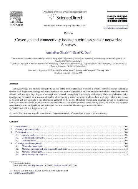
Fig. 2. (a) Different paths between A and B have different exposures. (b) Minimal exposure path for single sensor in a square sensing field. (c) 

Minimal exposure path for single sensor in a sensing field bounded by a convex polygon. 

This definition of exposure as given by Eq. (7) is a path-dependent value, and it provides valuable information 

about the worst-case coverage of a sensor field. Given two end-points A and B in the sensing field, different paths 

between them are likely to have different exposures, as shown in Fig. 2(a). The one which minimizes the value of 

integral E(p(t), t 1 , t 2 ) is called the minimal exposure path. 

As an illustration (see Fig. 2(b)), it is shown in [45] that the minimal exposure path between the two points P(1, −1) 

and Q(−1, 1) in a sensing field restricted within the square region |x| ≤ 1, |y| ≤ 1 and having only one sensor located 

at (0, 0), consists of three segments: (1) a straight line segment from P to (1, 0), (2) a quarter circle from (1, 0) to 

(0, 1), and (3) another straight line segment from (0, 1) to Q. The idea is that since any point on the dotted curve is 

closer to the sensor than any point lying on the straight line segments along the edges of the square, the exposure is 

more on the dotted curve. Also, since the length of the dotted curve is longer than the line segment, it would induce 

more exposure when an object travels along it, given that the time duration is the same in both the cases. This method 

can be extended to more generic scenarios when the sensing region is not necessarily a square, but a convex polygon 

v 1 , v 2 , . . . , v n , and the sensor is located at the center of the inscribed circle, as illustrated in Fig. 2(c). Let the two 

curves between points v i and v j of the polygon are described as: 

Γ i j = v i u i ◦ { u }} { 

i u i+1 ◦ { u }} { 

i+1 u i+2 ◦ · · · ◦ u { }} { 

j−2 u j−1 ◦ u j−1 v j (8) 

Γ i ′ 

j = v iu i−1 ◦ u { }} { 

i−1 u i−2 ◦ { u }} { 

i−2 u i−3 ◦ · · · ◦ u { }} { 

j+1 u j ◦ u j v j (9) 

where v i u i represents the straight line segment from point u i to v i , and u { }} { 

i u i+1 represents the arc on the inscribed 

circle between two consecutive points u i and u i+1 , whereas ◦ denotes concatenation, and all +/− operations are 

modulo n. It can be shown that the minimal exposure path between vertices v i and v j is one of the curves Γ i j and Γ 

i ′ 

j , 

whichever has less exposure. 

The above two methods for calculating the minimal exposure path can further be extended to the case of many 

sensors. To simplify, the problem is transformed from the continuous domain into a tractable discrete domain 

by using a grid [45]. The minimal exposure path is then restricted to straight line segments connecting any two 

consecutive vertices on the grid. This approach transforms the grid into an edge weighted graph, and computes the 

minimal exposure path using Djikstra’s single-source shortest path algorithm or Floyd–Warshal’s all-pair shortest path 

algorithm. In [60], a distributed localized algorithm based on variational calculus, and a grid-based approximation 

algorithm are used to find expressions for the minimal exposure path for the cases of single sensor and multiple 

sensors, respectively. 

Further to the methods of calculating the minimal exposure path, the Unauthorized Traversal problem proposed 

in [15] is relevant. The objective here is to find a path P that has the least probability of detecting a moving target when 

n sensors are deployed in the sensing field. According to the coverage model described in Section 3.1, the probability 

of not detecting a target at a point u by a sensor s is (1 − c u (s)). If the decision about a target’s presence is taken by a 

collaborative group of sensors using value fusion or decision fusion, then c u (s) can be replaced by D(u), where D(u) 

is the probability of consensus target detection using value fusion or decision fusion. Therefore, the net probability, 

G(P), of not detecting a target moving in the path P is the product of the probabilities of no detection at each point


Fig. 3. Unauthorized Traversal problem. 

Fig. 4. Obstacle modeling: energy distortion factor α i (u) due to the presence of obstacles. 

u ∈ P. Taking logarithm of G(P) this translates to: 

log G(P) = ∑ log(1 − D(u))du. (10) 

u∈P 

The algorithm divides the sensing field into a fine grid and assumes that the target moves only along the grid, as 

illustrated in Fig. 3. Since the exposure of P is 1 − G(P), finding the minimum exposure path on this grid is to find a 

path P that minimizes 1 − G(P), or equivalently that minimizes |log G(P)|. Consider two consecutive grid points, v 1 

and v 2 , and let m l denote the probability of not detecting a target traveling between v 1 and v 2 along the line segment l. 

Then, log m l = ∑ u∈P log(1 − D(u)). Each segment l is assigned a weight |log m l| and two fictitious points a, b, and 

line segments with zero weights are added from them to the grid points. Thus, the minimal exposure path in this configuration 

is to find the least weight path from a to b, which can be identified using Dijkstra’s shortest path algorithm. 

The concept of exposure as described so far is applicable only to stationary sensor networks, and does not 

incorporate the presence of obstacles. In contrast to that, a mobile sensor network, where both the nodes and the 

potential target may change locations at any time, the conventional computation methods are not suitable as they do 

not capture the sequential movement of nodes. The start time of a target traversal affects the exposure in a mobile 

network, while it does not have any effect in the stationary case. A target can intelligently plan its entrance and 

departure times to reduce the probability of detection if they can guess the movement strategy of the nodes. 

One of the recent works that captures these characteristics, and formally defines and evaluates exposure in a mobile 

sensor network using time expansion graphs is presented in [13]. The authors use a modified version of the sensing 

model to incorporate the presence of obstacles and noise, as given by the following equation: 

S ′ (s i , u) = α i(u)K 

d(s i , u) α , E(s i, u) = S ′ (s i , u) + N 2 i , (11) 

where K is the energy emitted by the target, α i (u) is the energy distortion factor due to obstacles, Ni 

2 is the noise 

energy, and S ′ (s i , u) is the target energy received by sensor s i . Obstacles are assumed to be circular in shape and each 

one is characterized by two radii, r 1 and r 2 , as shown in Fig. 4. Signals that are emitted by a target at location u,


Fig. 5. (a) Voronoi diagram of ten randomly deployed nodes. (b) Voronoi polygon for node S, constructed by drawing perpendicular bisectors of 

the lines connecting S and its neighbors. (c) Delaunay triangulation for the same set of nodes. 

and pass through or near an obstacle incur a distortion factor α i (u) before reaching the sensor s i . Consider the two 

cones formed by the target to the inner and outer circles. A node that lies within the inner cone beyond the obstacle 

has distortion factor α i (u) = 0, whereas if it lies outside the outer cone the distortion factor is one. Between the two 

cones, α i (u) increases linearly from 0 to 1 with distance r − r 1 , where r is the distance from the center of the obstacle 

to the line joining the target and the node. Noise is assumed to be additive white Gaussian (AWGN) with mean 0 

and variance 1, and is independent at each node. Using a value fusion approach with a threshold τ, the probability of 

detecting a target by all the n sensors is given by: 

( n∑ 

D(u) = Prob 

i=1 

( 

) 

Ni 2 + S ′ (s i , u) > τ 

) 

. (12) 

4.2. Maximal exposure path and maximal breach path 

The concept of maximal exposure path defined in [60] relates to the highest observability in a sensing field. A 

maximal exposure path between two arbitrary points in a sensing field is defined as the path following which the total 

exposure, as given by the integral in Eq. (7), is maximum. It can be interpreted as the path having the best quality of 

coverage. It is shown that finding a maximal exposure path is NP-hard by reducing it to the known NP-hard problem 

of finding the longest path in an undirected weighted graph. Several heuristics are proposed in [60] to achieve nearoptimal 

solutions under certain constraints, such as bounded object speed, path length, exposure value, and time of 

traversal. 

Another very similar concept to the worst-case coverage path is the maximal breach path. In [44], it is defined as 

the path through a sensing field, such that, the distance from any point on the path to the closest sensor is maximum. 

The structure of Voronoi diagram [47] is used to find such a maximal breach path. In two dimensions, the Voronoi 

diagram of a set of discrete points tessellates the plane into a set of convex polygons, such that all points inside a 

polygon are closest to only one point. In Fig. 5(a), ten randomly placed nodes divide the bounded rectangular region 

into ten convex polygons, referred to as Voronoi polygons. Any two nodes s i and s j are called Voronoi neighbors of 

each other if their polygons share a common edge. The edges of a Voronoi polygon for node s i , as shown in Fig. 5(b), 

are the perpendicular bisectors of the lines connecting s i and its Voronoi neighbors. 

Since by construction, the line segments of a Voronoi diagram maximize the distance from the closest sites, a 

maximal breach path lies along the Voronoi edges. An algorithm is described in [44] to find such a maximal breach 

path. A Voronoi diagram is first constructed from the location information of the nodes. Then, a weighted, undirected 

graph is constructed, where each node corresponds to a vertex, and an edge corresponds to a line segment in the 

Voronoi diagram. Each edge is given a weight equal to the minimum distance from the closest sensor. The algorithm 

then checks the existence of a path between two points using breadth first search, and then uses binary search between 

the smallest and largest edge weights in the graph to find a maximal breach path. Note the subtle difference between 

a maximal breach path and a minimal exposure path; the former is one that minimizes the exposure at any given point 

in time, whereas the latter does not focus on one particular time, rather it tries to minimize the exposure acquired 

throughout an entire time interval.

4.3. Maximal support path 


Alongside the concept of maximal exposure path, Meguerdichian et al. [44] also defined another measure of the 

best-case coverage, called the maximal support path. A maximal support path through a sensing field between two 

points is a path for which the distance from any point on it to the closest sensor is minimum. The difference between 

the two lies in the fact that a maximal support path focuses on a given time instant, whereas a maximal exposure 

path considers all the time spent during an object’s traversal. A maximal support path in a sensing field can be found 

by replacing the Voronoi diagram by its dual, the Delaunay triangulation, as shown in Fig. 5(c), where the edges of 

the underlying graph are assigned weights equal to the length of the corresponding line segments in the Delaunay 

triangulation. A Delaunay triangulation [47] is a triangulation of graph vertices, such that, the circumcircle of each 

Delaunay triangle does not contain any other vertices in its interior. Similar to the maximal breach path algorithm 

described earlier, the algorithm to find a maximum support path also checks for the existence of a path using breadth 

first search and applies a binary search. 

4.4. Delay in intrusion detection 

Until now, we have studied algorithms to find worst-case and best-case coverage paths exploiting the concept 

of exposure. Inherent to these algorithms is the assumption that the network is globally connected, and that once a 

target is detected by any of the sensors, the information can be forwarded to a sink. However, there are scenarios 

where the network gets disconnected due to battery depletion, environmental factors, and random deployment. Multihop 

communication, using which the sensors might forward the detection information to a sink, is also hindered by 

interference, multi-path fading, and shadowing effects, leading to temporarily disconnected-networks. Therefore, it is 

important to study the time delay for a mobile intruder to be detected by a sensor that has a connected-path to a sink. 

This problem is precisely studied in [16] by modeling the network using Percolation theory [8]. A range of node 

densities above a critical threshold, λ c > 0 is considered, such that a single giant unbounded cluster of connectednodes 

appears almost surely, and that all other existing clusters are finite. The distribution of the distance traveled by 

a moving target is analyzed until it comes within the sensing range of a node that lies within the giant component 

containing the sink. It is shown that the first contact distance (H any ) of a target moving in a straight line with any 

sensor, and the first contact distance (H gc ) with the giant component containing the sink can differ largely, and that 

if the node distribution follows a Poisson point process, then H any is exponentially distributed, and thus memoryless, 

whereas H gc is not. It turns out that the difference between these two distances is significant and the contact with the 

first node occurs much sooner than with a node connected to the giant component. 

To emphasize this gap between the two contact distances, a thinned version of the same sensing field is considered 

with some of the nodes randomly and independently removed. It is shown in simulation that H any is only affected very 

slightly, whereas the compliment of the distribution function H gc continues to decay much faster at large distances. 

One implication of this behavior is that, having some small fraction of the nodes disconnected from the largest 

component is much more degenerative to the network’s capability to successfully detect targets at the giant component, 

compared to the ability of a node to detect targets in a less dense network where all the nodes are still connected to the 

sink. It is also shown that the distribution of H gc over short distances is non-memoryless (the curve of P(H gc > x) is 

convex at the beginning), and that for longer distances it is an exponential random variable. The authors compare the 

time of contact with the giant cluster for various target mobility models; linear movement and Brownian motion being 

at the two extremes. As expected, linear motion is detected first and pure Brownian motion is detected last, whereas 

the intermediate two models, the random waypoint and the Brownian motion with drift, perform in between. 

5. Coverage exploiting mobility 

The second category consists of coverage schemes that exploit mobility to relocate nodes to optimal locations 

to maximize coverage. In some situations where terrain knowledge is available a priori, nodes could be placed 

deterministically, while in others, due to the large scale of the network or inaccessibility of the terrain, resorting to 

random deployment is perhaps the only option. However, as it turns out, random deployment often does not guarantee 

full coverage, resulting in accumulation of nodes at certain parts of the sensing field while leaving other parts deprived 

of nodes. Keeping this in mind, some of the deployment strategies take advantage of mobility to relocate nodes to


sparsely covered regions after an initial random deployment to improve coverage. This section describes several of 

these deployment algorithms. 

The first couple of algorithms described in Sections 5.1 and 5.2 are based on the notion of potential field and virtual 

forces, respectively, where the mobile nodes could spread out from an initial configuration in order to improve area 

coverage. The next three algorithms presented in Section 5.3 known as the VEC, VOR, and Minimax are based on the 

structure of Voronoi diagram in which nodes are relocated to fill up coverage holes. Then, we describe an incremental 

self-deployment algorithm in Section 5.4, and the Bidding protocol in Section 5.5; the latter one also uses Voronoi 

diagram but employs a combination of static and mobile nodes and the concept of bids to optimally relocate the mobile 

nodes to improve coverage. Next, in Section 5.6 we describe two schemes that consider nodes with limited mobility 

in order to achieve a trade-off between energy consumption and the density of nodes. Lastly, we discuss the concept 

of dynamic coverage in Section 5.7, which is useful in applications where not every part of the terrain is needed to be 

covered at all times, instead over a period of time the whole terrain needs to be swept at least once. 

5.1. Potential field-based 

In [30], a potential field-based deployment technique using mobile robots is proposed, while in [51], the scheme 

is augmented so that every node has at least K neighbors. The potential field technique using mobile robots is first 

introduced in [35]. 

The idea of potential field is that every node is subjected to a force F = −∇U that is a gradient of a scalar potential 

field U. Each node is subjected to two kinds of forces: (1) a repulsive force F cover that causes the nodes to repel each 

other, and (2) an attractive force F degree that constrains the node degrees from going too low by making them attract 

towards each other when they are on the verge of being disconnected. The forces are modeled as inversely proportional 

to the square of inter-node distances, and they obey the following two boundary conditions: 

– ‖F cover ‖ → ∞ when the distance between two nodes approaches zero to avoid collision, 

– ∥ ∥ Fdegree 

∥ ∥ → ∞ when the distance between neighboring nodes approaches Rc , the communication radius. 

In mathematical terms, if d(s i , s j ) is the Euclidean distance between two nodes s i and s j that are located in x i and 

x j , and ˆn ij represents the unit vector along the line joining the two nodes then, F cover (i, j) and F degree (i, j) can be 

expressed as: 

F cover (i, j) = −K cover 

d(s i , s j ) 2 ˆn ij (13) 

⎧ 

⎨ −K degree 

[ ] 

F degree (i, j) = 

2 ˆn ij , for critical connection 

⎩ d(si , s j ) − R c 

0, otherwise. 

(14) 

In the initial configuration all the nodes are accumulated in one place, possibly at the center of the sensing field, 

and therefore, each node has at least K neighbors (assuming the total number of nodes to be more K ). Then, they 

start repelling each other using F cover until each node has only K neighbors left, at which point the connections reach 

a critical threshold, none of which should be broken to ensure K -connectivity. Each node continues to repel all its 

neighbors using F cover , but as the distance between a node and its critical neighbors increases, F cover decreases and 

F degree increases. Finally, at some distance, cR c , where 0 < c < 1, the net force ∥ ∥F cover + F degree 

∥ ∥ becomes zero, 

and the nodes reach an equilibrium, thus covering the sensing field uniformly. At a later point, if a new node joins the 

network or an existing node ceases to function, the nodes will need to reconfigure to satisfy the equilibrium criteria. 

5.2. Virtual force-based 

Similar to the potential field-based approach, a sensor deployment technique based on virtual forces is proposed 

in [74] and [73] to increase the area coverage after an initial random deployment. In this model, each node s i is 

subjected to three kinds of forces: (1) a repulsive force F i R , exerted by obstacles, (2) an attractive force F i A , exerted 

by areas of preferential coverage (sensitive areas where a high degree of coverage is required), and (3) an attractive 

or repulsive force F i j , by another node s j depending on its distance and orientation from s i . A threshold distance


d th is defined between two nodes to control how close they can get to each other. Likewise, a threshold coverage c th 

is defined for all grid points such that the probability of a target at any grid point being detected is greater than this 

threshold. The coverage model as described in this algorithm is given by Eqs. (2) and (3). The net force on a sensor s i 

is the vector sum of all the above three forces: 

F i = F i R + F i A + 

k∑ 

j=1, j≠i 

F i j . (15) 

Once the nodes are randomly deployed in the sensing field, the algorithm calculates the total coverage as defined 

by Eq. (3) for all the grid points. Then it calculates the net virtual force exerted on each sensor s i by all other sensors, 

obstacles, and preferential coverage areas. Depending on the net force, new locations are calculated by a cluster head 

and a one-time movement is performed by the nodes to their designated locations. Negligible computation time and 

one-time repositioning of nodes are two of its primary advantages. However, for relocating nodes the algorithm does 

not provide any route plan to avoid collision. 

Along the lines of potential field and virtual force-based techniques, a distributed self-deployment algorithm is 

proposed in [27] for mobile sensor networks that maximizes coverage and maintains uniformity in node distribution. 

It defines coverage as the ratio of the union of covered areas by each node to the total area of the sensing field; and 

uniformity as the average of standard deviations of inter-nodal distances. In uniformly distributed networks, internodal 

distances are almost the same, and therefore, the energy consumption is uniform. It assumes that the initial 

deployment is random and that each node knows its location. Similar to the virtual force algorithm, it also uses the 

concept of electric forces that depend on inter-node separation and local current density, µ curr . At the beginning, the 

initial density for each node is equal to the number of its neighbors. The algorithm defines the notion of expected 

density as the average number of nodes required to cover the entire area when the nodes are deployed uniformly. It is 

given by µ(R c ) = nπ R2 c 

ξ 

, where n is the number of sensors, R c is the communication radius, and ξ is the area. The 

algorithm executes in steps and models the force on the ith node exerted by the jth node at time step t as: 

f i, j 

t = µ curr ( 

Rc 

µ 2 − ∣ xi (t) − x j (t) ∣ ) ˆn ij (t) (16) 

(R c ) 

where x i (t) denotes the location of ith node at time t, and ˆn ij (t) represents the unit vector along the line joining the 

two nodes at time t. Depending on the net forces from the neighborhood, a node can decide on its next movement 

location. The algorithm settles down when a node moves an infinitely small distance over a period of time or when it 

moves back and forth between two same locations. 

5.3. VEC, VOR, and MiniMax 

In [63], three distributed self-deployment algorithms known as VEC, VOR, and MiniMax are proposed for mobile 

sensor networks that exploit the structure of Voronoi diagrams. As noted before, a Voronoi diagram consists of Voronoi 

polygons with the property that all points inside a polygon are closest to the node that lies within the polygon. The 

common strategy in all these three algorithms is that once the Voronoi polygons are constructed, each node within 

its polygon finds out the existence of possible holes and relocates itself to the new positions in order to reduce or 

eliminate the coverage holes. 

The vector-based algorithm, VEC, pushes nodes away from densely covered areas to sparsely covered areas. Two 

nodes exert a repulsive force when they are too close to each other. If d avg is the average distance between any two 

nodes when they are evenly distributed in the sensing field, the virtual force between two nodes s i and s j will move 

each of them d avg−d(s i ,s j ) 

2 

distance away from each other. However, if one of the node’s sensing range completely 

covers its Voronoi polygon, then only the other node moves away a distance d avg − d(s i , s j ). In addition to the mutual 

repulsive forces between nodes, the boundaries also exert forces to push nodes inside that are too close to the boundary. 

If d b (s i ) is the distance of node s i from its closest boundary, the repulsive force moves it a distance d avg 

2 

− d b s i 

towards the inside of the region. Before actually moving to the new position, however, each node calculates whether 

its movement would increase the local coverage within its Voronoi polygon. If not, the node refrains from moving to 

the target location, instead, it applies a movement adjustment scheme and will move to the midpoint position between 

its target location and the new location.


Fig. 6. (a) The VOR algorithm moves a node towards the farthest Voronoi vertex, V far (b) Bid estimated by node S i is the area of the shaded circle 

with center at C. 

Fig. 7. (a) Environment with obstacles and a single sensor, (b) Occupancy grid: black cells are occupied, gray ones are unknown and white ones 

are free, (c) Configuration grid: black cells are occupied, gray ones are unknown and white ones are free, (d) Reachability grid: white cells are 

reachable, gray ones are unknown. 

VOR is a greedy strategy that pulls nodes towards the locations of their local maximum coverage holes. If a node 

detects a coverage hole within its Voronoi polygon, it will move towards its farthest Voronoi vertex, V far , such that 

the distance from its new location, A, to V far is equal to the sensing radius (see Fig. 6(a)). However, the maximum 

moving distance for a node is limited to at most half the communication radius, because the local view of the Voronoi 

polygon might be incorrect due to limited communication range. VOR also applies the movement adjustment scheme 

as in VEC, and additionally applies an oscillation control scheme that limits a node’s movement to opposite directions 

in consecutive rounds. 

The MiniMax algorithm is very similar to VOR; it moves a node inside its Voronoi polygon, such that, the distance 

from its farthest Voronoi vertex is minimized. Since moving a node to its farthest Voronoi vertex might lead to a 

situation that the vertex which was originally close now becomes a new farthest vertex, the algorithm positions each 

node such that no vertex is too far away from the node. It defines the concept of a Minimax circle, the center of which 

is the new targeted position. To find the Minimax circle, all circumcircles of any two and any three Voronoi vertices 

are found and the one with minimum radius covering all the vertices is the Minimax circle. 

5.4. Incremental self-deployment 

In [29] and [28], an incremental and greedy self-deployment algorithm is presented for mobile sensor networks 

in which nodes are deployed one at a time into an unknown environment. Each node makes use of the information 

gathered by previously deployed nodes to determine its optimal deployment location. The algorithm ensures maximum 

coverage and guarantees line of sight between nodes. Conceptually, it is similar to the frontier-based approach [68]; 

however, in this case, occupancy maps are built from live sensory data and are analyzed to find frontiers between the 

free space and the unknown space. 

In the Initialization phase, nodes are assigned one of the three states: waiting, active or deployed with the exception 

of a single node that acts as an anchor and is already deployed. 

In the next phase called the Goal Selection phase, an optimal location is chosen for the next node to be deployed 

based on previously deployed sensors. The concept of occupancy grid [17] as shown in Fig. 7(b) is used as the first step


to global map building. Each cell is assigned a state of either free (known to contain no obstacles), occupied (known to 

contain one or more obstacle) or unknown. However, not all free space represent valid deployment locations because 

nodes have finite size and a free cell that is close to an occupied cell may not be reachable. Hence, the occupancy grid is 

further processed to build a configuration grid as in Fig. 7(c). In a configuration grid, a cell is free if all the occupancy 

grid cells lying within a certain distance are also free. A cell is occupied if there are one or more occupancy grid cells 

lying within a certain distance are similarly occupied. All other cells are marked as unknown. Once this global map is 

built, the goal selection phase chooses a location based on certain policies. 

Next, this new location is assigned to a waiting node in the Goal Resolution phase and a plan for reaching the goal 

is generated applying a distance transform (also called flood-fill algorithm) on the configuration grid, giving rise to a 

reachability grid as depicted in Fig. 7(d). Thus, the set of reachable cells is a subset of the set of free configuration 

cells, which in turn is a subset of the set of free occupancy cells. A distance of 0 is assigned to the goal cell (which is 

chosen to be the optimal location for the next node to be deployed), a distance of 1 to cells adjacent to the goal cell, a 

distance of 2 to their adjacent cells and so on. However, distances are not propagated through occupied or unknown 

cells. Thus, for each node the distance to the goal and whether or not the goal can be reached is determined. 

In the Execution phase, the active nodes are deployed sequentially to their respective goal locations. The nodes end 

up moving in a ‘Conga Line’, i.e., as the lead node moves forward, the node immediately behind it steps forward to 

take its place; this node in turn is replaced by the one behind it and so on. 

5.5. Bidding protocol 

The algorithms described in the previous sections apply to networks where all the nodes are capable of moving 

around. However, there is a high cost associated to make each node mobile; a balance can be achieved by using a 

combination of static and mobile nodes, usually referred to as hybrid sensor networks, while still ensuring sufficient 

coverage. In [62], such a protocol is described, called the bidding protocol, where the problem is reduced to the 

well-known NP-hard set-covering problem. A heuristic is also proposed to solve it near optimally. 

In the proposed algorithm, initially, a fixed of static and mobile nodes are randomly deployed in the sensing field. 

Then, a Voronoi diagram is constructed using only the static nodes, which then find the existence of possible holes 

within their respective polygons, and also bid to the mobile nodes to move to the locations of the holes. If a hole is 

found, a static node chooses the location of the farthest Voronoi vertex as the target location for the mobile node and 

calculates the bid as π(d − R s ) 2 , where d is the distance between the node and the farthest Voronoi vertex as shown 

in Fig. 6(b). A static node then finds the closest mobile node whose base price (each mobile node has an associated 

base price which is initialized to zero) is lower than its bid and sends out a bidding message. A mobile node receives 

all such bids from its neighboring static nodes, chooses the highest bid, and moves to heal the corresponding coverage 

hole. The accepted bid becomes the mobile node’s new base price. This approach ensures that a mobile node does 

not move to heal a coverage hole when its movement generates a larger hole in its original place. The protocol also 

incorporates a self-detection scheme to ensure that no two mobile nodes move to heal the same coverage hole. It also 

applies the movement adjustment scheme similar to VEC, to push away nodes from each other if their movement can 

result in more coverage. 

As mentioned earlier, the deployment of nodes in a hybrid sensor network requires a balance between the number of 

static and mobile nodes. Thus, instead of always deploying a fixed number of nodes, it could be useful to dynamically 

estimate the number of additional mobile nodes required to improve coverage. In [21], initially a fixed number of 

static nodes are deployed that deterministically find out the exact amount of coverage holes existing in the entire 

network using the structure of Voronoi diagrams, and then dynamically estimate the additional number of mobile 

nodes needed to be deployed and relocated to the optimal locations of the holes to maximize overall coverage. This 

approach of deploying a fixed number of static nodes and a variable number of mobile nodes can provide optimal 

coverage under controlled cost. A hybrid sensor approach is a very attractive one, because it allows one to choose the 

degree of coverage required by the underlying application as well as gives an opportunity to optimize on the number 

of additional mobile nodes. 

5.6. Coverage with limited mobility 

The schemes discussed so far do not have any restriction on the mobility of the nodes, in the sense that a mobile 

node could travel as much as needed by the algorithm. This poses three disadvantages: (1) mobility consumes more


energy than communication or sensing, (2) redeployment process might take considerable amount of time in large 

networks because of the limited speed of the mobile nodes, and (3) the maximum movement distance of a node might 

be limited [41]. To this end, the works described in [64] and [11] consider deployment strategies with limited mobility, 

where nodes could move only over a short distance. 

In [64], a trade-off between the mobility and density of nodes is analyzed in terms of a metric defined as the 

over-provisioning factor, where the mobile nodes are further restricted to move only once. For a given deployment 

strategy, the over-provisioning factor is defined as the ratio of the node density (λ) and the degree of coverage (k), 

i.e., λ/k. Intuitively, this metric indicates the efficiency of a network deployment strategy and is lower bounded 

by Θ(1). This lower bound can be achieved with deterministic placement using only static nodes, or with random 

deployment using all mobile nodes by relocating them to optimal locations without any restriction on their mobility. 

However, for random deployment with static nodes the metric scales as Θ( log A 

k 

+ log log A), where A is the area of 

the sensing field, thus, resulting in low efficiency for large networks. Under the setting of random deployment and 

limited mobility, it is shown using the results of the minimax grid matching problem [37] that a network can achieve an 

over-provisioning factor of π/2 with the maximum distance traveled by any mobile node equal to O( √ 1 log 3/4 (k A)) 

k 

with high probability. Thus, it is possible to achieve constant over-provisioning factor, as in the case of deterministic 

placement, by relocating mobile nodes only once over a short distance. Furthermore, it is shown that even for a hybrid 

network comprising both static and mobile nodes, an O(1) over-provisioning factor is achievable with a maximum 

distance traveled by any mobile node equal to O(log 3/4 A) with high probability, while the fraction of mobile nodes 

required is less than 1/ √ 2πk. A distributed algorithm is also proposed to optimally relocate the mobile nodes using 

the formulation of a minimum cost network flow problem. 

In many applications, certain regions of the environment might be required to be sensed with a high sampling rate, 

such as structural health monitoring networks. However, due to hardware limitations, a single sensor per region might 

be insufficient to perform such high sampling measurements. Moreover, there could be obstacles or external factors 

like heat, vibration, etc. that can hinder sensing ranges. Such sensing dynamics can be compensated with multiple 

sensors per region. The work described in [11] addresses this problem, where the objective is to determine a sequence 

of optimal sensor movements under limited mobility in order to guarantee the required number of nodes at certain 

regions of the sensing field. The challenge here is to simultaneously minimize the total number of movements as well 

as the total variance in the number of nodes from the prescribed number. A centralized algorithm is proposed that 

models the above problem as a minimum cost maximum weighted flow in a graph constructed by assigning appropriate 

weights to the regions and costs to the edges that represent accessibility between regions, and it is shown that this flow 

can be translated as the optimal sensor movement plan that minimizes the variance and sensor movements. 

The deployment strategies discussed so far strive to relocate and spread sensors from an initial static configuration 

in order to maximize coverage. The main difference among these algorithms is how exactly the new positions are 

computed. However, one drawback is that the final network configuration is again static, and therefore, parts of the 

sensing field that are still uncovered even after the relocations will remain so. As a consequence, an intruder moving 

along those uncovered regions will never get detected. In addition, static sensor networks are also not able to cope 

with dynamic environments where new obstructions may appear after the initial deployment. To overcome these 

drawbacks, the concept of dynamic coverage is introduced as described below. 

5.7. Dynamic coverage 

There have been considerable amount of research efforts using mobile sensors that can patrol the environment 

in order to provide better quality of coverage and detection capability. The quality of coverage by mobile sensors 

depends on the velocity, mobility patterns, number of sensors deployed, and the dynamics of the phenomenon being 

sensed. It is to be noted that although a mobile sensor is able to cover more area than a stationary sensor over a period 

of time, the instantaneous area covered by both are the same. Hence, proper motion planning is required to exploit the 

full advantage of mobile sensors. The works presented in [40,7,64], and [11] address these issues. 

5.7.1. Event detection: Sensor strategy vs. target strategy 

In [40], the dynamic aspects of coverage exploiting mobility are studied. When a bunch of mobile nodes roam 

around in the sensing field, uncovered areas are more likely to get covered over time, and intruders that might never 

have been detected in stationary networks can now be detected by the mobile sensors (see Fig. 8). This scenario is of


Fig. 8. Coverage due to node mobility: The left figure shows the initial static configuration at time 0, and the right figure shows the effect of node 

mobility during time interval [0, t). The union of the shaded regions and the solid disks represents the area being covered during the time interval. 

great importance to applications that do not require simultaneous coverage of all the locations at specific times, but 

require overall greater coverage over a period of time. In [7], it is investigated how the quality of coverage depends 

on parameters such as, sensor speed, event dynamics, and the number of sensors deployed. A scenario is considered 

where events can appear and disappear at certain known points, called Points of Interest (PoIs), within the monitoring 

region, and the goal is to detect the events using mobile sensors. Additionally, optimal and heuristic path planning 

algorithms are presented for the Bounded Event Loss Probability (BLEP) problem, i.e., to plan sensor motion such 

that the probability of the event not being detected is bounded from above. 

Assuming that the static distribution of nodes in the two-dimensional plane is a Poisson point process [57] with 

density λ, and the sensing model is a binary disk of radius R s , the fraction of the region covered by at least one sensor 

at time t > 0 is shown in [40] to be given by: 

f stationary (t) = 1 − e −λπ R2 s . (17) 

However, if the nodes move around in the sensing field following a random mobility model, then the fractional area 

coverage during a given time interval [0, t) is given by: 

f mobile (t) = 1 − e −λ( π R 2 s +2R s E[V s ]t ) , (18) 

where E[V s ] represents the expected sensor speed. Analytic expressions are derived in [40] for the detection time of 

both static and mobile targets. In particular, if the sensors move according to a random mobility model with fixed speed 

v s , then the detection time for a stationary target follows an exponential distribution with mean 1/2λrv s . On the other 

hand, if the target is also moving at speed v t along direction θ t , then the detection time also follows an exponential 

distribution with parameter 1/2λrv¯ 

s , where v¯ 

s is the effective sensor speed relative to the target. We observe that the 

detection times of both stationary and moving targets follow exponential distributions with parameters of the same 

form. Thus, maximizing the detection time corresponds to minimizing the effective sensor speed. It is also shown that 

the optimal target movement strategy for minimizing detection time when the sensors move in the same direction is 

also to move in the same direction as the sensors at a speed closest matching to the sensor speed, and the corresponding 

detection time is 1/2λr(v s − vt 

max ), where vt 

max is the maximum target speed. However, if the sensor movement is 

uniformly chosen within [0, 2π), then the maximum expected detection time is achieved when the target does not 

move, and thus the expected detection time is 1/2λrv s . The latter result could be intuitively explained as follows. 

Since the sensors move in all directions with equal probability, the movement of the target in any direction will result 

in a higher effective speed with respect to the sensor, and therefore will be detected faster. 

The quality of coverage metric for the analysis presented in [7] is the fraction of events captured by mobile sensors, 

where the events occur at the PoIs scattered along a simple closed curve C as shown in Fig. 9(b). A mobile sensor is 

able to sense an event occurring at a PoI if the distance between the sensor and the PoI along C is less than its sensing 

radius R s . To capture event dynamics, each PoI is modeled as a continuous-time Markov chain (see Fig. 9(a)) that 

alternates between two states 0 and 1, where state 1 corresponds to an event being present and state 0 corresponds to no 

event. The time spent by all PoIs in states 0 and 1 are exponentially distributed with means 1/λ and 1/µ, respectively. 

Based on this framework, three different mobile sensor deployment scenarios are considered: (1) single sensor 

moving with constant velocity v, (2) multiple sensors moving with fixed velocity v, while remaining equidistant from 

each other, and (3) single sensor moving with variable speed lying between 0 and v max . For each of these scenarios,


Fig. 9. (a) The two-state continuous-time Markov chain for each Point of Interest (PoI). (b) PoIs scattered along a curve C and a mobile sensor 

moving along the curve to detect events occurring at the PoIs. 

expressions for the expected fraction of events detected are derived as a function of event dynamics (λ, µ) and sensor 

parameters, v and R s . For the first case, the number of events captured by a mobile sensor during its visit depends on 

the state of the PoI at the beginning of the visit and the number of state cycles, transitions of the form 0 → 1 → 0 or 

1 → 0 → 1, during the visit. The analytical results suggest that for a given event dynamics (λ, µ), there is a critical 

velocity above which a mobile sensor is able to capture more events compared to a stationary sensor, whereas below 

it the probability of detection is lower than using a stationary sensor placed at any one of the PoIs. This is because, 

intuitively a slow sensor spends most of the times traveling around regions of C where no PoIs can be seen (futile 

regions). Higher velocity enables a sensor to cover these futile regions in shorter time. This critical velocity increases 

as the rate of events appearing (λ) and disappearing (µ) increases. 

For the case of multiple sensors, it is observed that the gain in the event detection probability is not commensurate 

with the increase in the number of sensors after a certain threshold. The gains of mobility are higher when the number 

of sensors deployed are less. It is also observed that the gains of increasing number of sensors diminish with higher 

speed. These results provide guidelines for choosing the velocity and the number of sensors to be deployed for 

satisfying constraints on the fraction of events captured. Lastly, for the case of single sensor with variable speed, 

it is intuitive that to maximize the fraction of events captured a mobile sensor should slow down and move at a speed 

v c ∈ (0, v max ] (called capture speed) when it is within the 2R s distance from a PoI, and at the maximum speed v max 

while moving in the futile regions. However, there is a trade-off between slowing down and maximizing the number 

of events captured. This is because if there is a large number of PoIs spread apart from each other where events can 

occur, then slowing down in the vicinity of a particular PoI implies that the sensor might miss a large number of 

events taking place at other PoIs. In general, the best policy for the sensor is to keep moving at maximum possible 

speed. 

5.7.2. Bounded event loss probability problem 

In [7], a second metric is also investigated to measure the quality of coverage in terms of event loss probability 

through the BELP problem. If a given PoI i (i = 1, 2, . . . , a) has event dynamics (λ i , µ i ) and is located at point 

P i , then the goal of the BELP problem is to generate a motion plan for the mobile sensors, such that the probability 

that an event occurring at i is not captured by any of the mobile sensors is less than some ɛ > 0. Note that the 

constraint on miss-probability is a stronger condition than the fraction of events captured. The BELP problem is posed 

as two different versions: (1) Minimum Velocity BELP (MV-BELP), where given a set of PoIs, their locations and 

event dynamics, the goal is to find the minimum velocity required for a mobile sensor to satisfy the miss-probability 

constraint, and (2) Minimum Sensors BELP (MS-BELP), where the goal is to find a minimum number of mobile 

sensors, each moving with velocity v, that need to be deployed to satisfy the constraint, given the same input as (1). 

Both of these versions turn out to be NP-hard. The MV-BELP problem basically requires finding an optimal path 

that the mobile sensor must take to visit the PoIs, such that the time elapsed between two consecutive visits to a 

particular PoI is no less than a critical time that is required to satisfy the probability constraint. This is in essence the 

Traveling Salesman Problem (TSP) [5], which is known to be NP-hard. On the other hand, the MS-BELP problem 

or v = 0 is reduced to the minimum set cover problem, which is again NP-hard. Heuristics are proposed in [7] for


special deployment scenarios of the PoIs, such as when they are deployed linearly, on a closed curve, and on the twodimensional 

plane. These results can be applied to a wide range of application scenarios that involve arrival of events 

at spatially distributed points, which have to be sensed/served within a bounded time, e.g., surveillance applications, 

underwater networks, and supply chain management. 

6. Integrated coverage and connectivity 

Our discussion so far has primarily dealt with algorithms that guarantee optimal coverage of a sensing field. 

However, for a sensor network to operate successfully the nodes must also form a connected-network so that the 

sensed data can be transmitted in multi-hop to other nodes and possibly to a base station where intelligent decisions 

can be made. Therefore, it is equally important for a coverage algorithm to ensure network connectivity. 

One of the fundamental results concerning integrated coverage and connectivity states that the following. 

Theorem 1. If the communication radius of a node is at least twice the sensing radius, i.e., R c ≥ 2R s , then 

1-coverage of a convex region is sufficient to guarantee 1-connectivity of the network [65,69]. 

Thus, under this condition, a sensor network only needs to be configured to guarantee coverage because 

connectivity will be intrinsic. Extending this basic result it is also shown in [65] that under this condition, k-coverage 

of a convex region implies k-connectivity among all the sensors, and 2k-connectivity among the internal sensors 

(whose sensing circle does not intersect the boundary of the convex deployment region). 

In this section, we describe several schemes that are similar in spirit in terms of ensuring a connected-coverage of 

a sensing field, while reducing redundancy and increasing overall network life time. We divide these deployment 

into two categories: (1) that are based on regular patterns, and (2) that are based on sleep scheduling. First, 

we describe several pattern-based deployments for two dimensions in Section 6.1.1 and for three dimensions in 

Section 6.1.2. The sleep schedule-based techniques are described in Section 6.2, under which, in Section 6.2.1 we 

first describe algorithms that select to activate an optimal number of nodes to provide a connected-coverage, and next 

in Section 6.2.2 we discuss algorithms that find trade-offs between coverage, latency, and energy consumption without 

necessarily guaranteeing complete coverage of the region. 

6.1. Connected-coverage by pattern-based deployment 

6.1.1. Two-dimensional case 

In practice, sensor networks are often deployed in two-dimensional plane following regular patterns due to the 

convenience of deployment and higher degree of connectivity, such as the hexagon, square grid, rhombus, and 

equilateral triangle. On the problem of achieving both coverage and connectivity at the same time, it is important 

to investigate optimal deployment patterns for general values of the ratio of the communication radius to the sensing 

radius, R c /R s . The authors in [34] focus on the case when R c /R s = 1, and develop a necessary condition on the 

spatial density of nodes required for an optimal topology that provides connected-coverage of the two-dimensional 

plane. It is shown that the node density required by the optimal topology is given by: 

d OPT ≥ 0.522 

r 2 . (19) 

This optimal node density is used to access the efficiency of several deployment patterns such as the square-, 

hexagon-, and strip-based deployment. In particular, the density of nodes in a square-grid is given by d SQ R = 1/Rs 2, 

while for a hexagonal-grid is given by d HEX = 0.769/Rs 2 . Comparison of these expressions with Eq. (19) shows that 

the density required for the square topology is roughly twice the optimal and that of the hexagonal grid is roughly 1.5 

times the optimal. On the other hand, the strip-based deployment, described below, provides a near-optimal density of 

nodes with d STR = 0.536/Rs 2. 

Consider a string of sensors (strip) arranged in a horizontal line with inter-node spacing equal to R s . Since R s = R c , 

this forms a connected-component (see Fig. 10(a)). Next, imagine arranging these strips in the following manner. For 

√ 

every integer k place a strip horizontally such that there is one node positioned at (0, k( 3 

2 + 1)R s) for every even k, 

√ 

and one node positioned at (R s /2, k( 3 

2 + 1)R s) for every odd k. Finally place some nodes vertically in the following


Fig. 10. (a) A connected-strip-based topology: small dark dots represent sensor nodes and circles represent their sensing/communication radii; the 

lines represent the edges of the connectivity graph. Not all the circles are shown. (b) A truncated octahedron. 

√ 

way. For every odd k, place two nodes at (0, k( 3 

2 + 1)R s ± 

2 

). The purpose of this vertical strip is to connect the 

horizontal strips and thus ensure connectivity between all nodes. 

Extending the above work, which is only applicable for R c /R s = 1, an optimal deployment pattern is proposed 

in [6] to achieve both full coverage and 2-connectivity of a square region. The optimality of the algorithm is proved 

for all values of R c /R s . The authors also proved the asymptotic optimality of the strip-based algorithm described 

above for full coverage and 1-connectivity for all R c /R s < √ 3. The new deployment pattern is a variant of the 

strip-based topology and can be constructed as follows. As before, a horizontal strip of sensors is formed by placing 

nodes on a line at regular intervals with separation φ h = min{R c , √ 3R s }. These strips are then deployed horizontally 

with alternate rows √ shifted to the right by a distance φ h /2. The vertical separation between two neighboring strips 

is φ v = R s + Rs 2 − φ2 h /4. Note that, when R c/R s < √ 3, the neighboring strips are not connected. In this 

case √ additional nodes are placed at the left and right boundary of the deployment region with inter-node separation 

φh 2/4 + φ2 v . 

Besides proving the optimality of the modified strip-based pattern for full coverage and 2-connectivity, several 

regular deployment patterns, such as hexagon, square grid, rhombus, and equilateral triangle are also compared in [6] 

with respect to the number of nodes required for a range of values of R c /R s . The metric used to compare their 

efficiency is the area of the Voronoi polygons formed by these patterns. Note that, for a given regular pattern all 

the Voronoi polygons have the same area. It can be shown that the maximum areas of the Voronoi polygons for the 

hexagon (γmax H ), square (γ max S ), and triangular patterns (γ max T ) are given by the following: 

γ H max = 3 4√ 

3 (min{Rc , R s }) 2 (20) 

{ 

γmax (min 

S = 2 R s , R c / √ 2 

2}) 

(21) 

γ T max = 3 2 

√ 

3 

√ ( { 

3 min R s , R c / √ 2 

3}) 

. (22) 

The corresponding expression for the rhombus pattern is: 

γ R = 

( { 

min R c , 2R s cos θ }) 2 

sin θ. (23) 

2 

The maximum value occurs at θ = π/2 when R c /R s ≤ √ 2, at θ = π − 2 sin −1 (R c /2R s ) when √ 2 ≤ R c /R s ≤ √ 3, 

and at θ = π/3 when ≤ R c /R s . Based on the above expressions the four deployment patterns are compared, and the


best-pattern results by choosing the one for which γ max is one of the following depending on the value of R c /R s : 

⎧ 

γmax ⎪⎨ 

H , when 0 < R c/R s ≤ 1 2 33/4 

γ max = γmax S , when 33/4 ≤ R c /R s ≤ √ 2 

γmax ⎪⎩ 

R , when √ 2 ≤ R c /R s ≤ √ (24) 

3 

γmax T , when √ 3 ≤ R c /R s . 

Note that the above algorithms are based on the oversimplified binary disk model for both sensing and 

communication. In reality, however, the sensing and communication ranges hardly follow a disk model. The problem 

of determining optimal deployment patterns that use statistical models of sensing and communication to make 

probabilistic guarantees on coverage and connectivity is still open. 

6.1.2. Three-dimensional case 

Majority of the literature till date have focused on modeling wireless terrestrial networks in two-dimensions. 

However, the recent growing interest in underwater acoustic networks [59] for marine life and coral reef monitoring, 

and atmospheric networks for weather forecasting and climate monitoring necessitates us to understand threedimensional 

(3D) networks. Unfortunately, the design of three-dimensional networks is surprisingly more difficult [50] 

that its two-dimensional counterpart, and consequently there are only a limited number of works in the literature that 

deal with such networks. In [2], the problem of coverage and connectivity in three-dimensional networks is addressed, 

where the goal is to find a node placement strategy with 100% sensing coverage of a three-dimensional space while 

minimizing the number of nodes. This work is based on the Voronoi tessellation of three-dimensional space, and it 

uses Kelvin’s conjecture [66], which asks the following question: what is the optimal way to fill a three-dimensional 

space with cells of equal volume, such that the surface area (interface area) is minimized This essentially amounts to 

finding a space-filling structure with the highest isoperimetric quotient, defined as 36π V 2 /S 3 , where V is the volume 

and S is the surface area of a cell. Sphere has the highest isoperimetric quotient of 1, however, it does not tessellate a 

three-dimensional space. Kelvin’s answer to this question is the 14-sided truncated octahedron with a slight curvature 

of the hexagonal faces and isoperimetric quotient of 0.757. 

Assuming that the sensing region of a node is a spherical ball of radius R s , the problem is to find a lattice structure 

such that when the nodes are placed at the circumcenter of the lattice cells, there is minimum overlap among the 

sensing regions and there is no point which is uncovered. This in turn implies finding a minimum number of nodes to 

fill a three-dimensional space. A space-filling polyhedron 1 is a polyhedron that can be used to fill a volume without 

any overlap or gap (tessellation). Unfortunately, spheres do not tessellate in three-dimensional, and so the goal is to 

find a space-filling polyhedron that best approximates the sphere. Note that, it is not easy to show that a polyhedron 

has space-filling property. Among the five regular polyhedrons (platonic solids) – cube, dodecahedron, icosahedron, 

octahedron, and tetrahedron – only the cube has the space-filling property. In addition, some combinations of these 

solids also fill space. 

Based on Kelvin’s conjecture, the uncurved truncated octahedron (see Fig. 10(b)) with an isoperimetric quotient 

of 0.753367 is proposed in [2] as the optimal lattice to the coverage problem in three-dimensional space in terms of 

minimum number of nodes. A truncated octahedron has 14 faces, of which 8 are hexagonal and 6 are square, and the 

length of the edges of hexagons and squares are the same. The transmission range required to maintain connectivity 

among neighboring nodes in this case is 1.7889R s . 

Before moving on to the sleep scheduling-based algorithms, it is worth mentioning that the coverage problem in 

three-dimensional networks addressed in [32] is formulated as a decision problem, where the goal is to determine 

whether every point in the region is covered by at least k sensors. The basic idea is to reduce the geometric problem 

from a three-dimensional space to a two-dimensional space by observing that the region is divided into a number of 

subspaces by the spherical ball of each node, and that the level of coverage of a subspace can actually be derived 

from the spherical segments that comprise the subspace. Furthermore, each spherical segment must be bounded by 

a number of circle segments, and the level of coverage of a spherical segment can actually be derived from those 

1 A polyhedron is a three-dimensional shape consisting of finite number of faces, e.g., cube, prisms, pyramids etc. A polygon is a two-dimensional 

analog of a polyhedron. The generic term for any dimension is a polytope.


of its circle segments that bound the spherical segment. This transforms the two-dimensional problem into a onedimensional 

problem, and therefore, it implies that to determine how a region is covered, it is sufficient to determine 

how each circle segment is covered. 

6.2. Connected-coverage by optimal sleep scheduling 

Many sensor network applications (e.g., data gathering) require a large number of nodes to be deployed with 

high density. In such applications it is often undesirable to keep all the nodes active at the same time in order to 

avoid excessive collisions and redundant sensing due to spatio-temporal correlation in measurements. Keeping all the 

nodes active simultaneously would also dissipate energy at a faster rate and reduce the network lifetime. A significant 

amount of energy savings can be achieved by turning off some nodes, thus eliminating redundant data and maximizing 

the time interval of continuous-monitoring, transmitting, or receiving. Such techniques, known as sleep scheduling 

schemes, that control the density of active nodes in sensor networks have been the focus of many research works. In 

these direction, both random and synchronized, as well as deterministic sleep scheduling schemes are proposed for 

certain scenarios. The main focus of these algorithms is to maintain sufficient coverage and connectivity, as desired 

by the application, by duty-cycling nodes in an optimal manner. We divide this set of algorithms into two fundamental 

categories: (1) that activates an optimal number of nodes to provide a complete connected-coverage, and (2) that finds 

optimal trade-offs between coverage and latency. 

6.2.1. Activating optimal number of nodes 

We noted in Theorem 1 that when R c ≥ 2R s a sensor network only needs to be configured for guaranteeing 

coverage because connectivity will be intrinsic. Based on these fundamental results a coverage configuration protocol 

(CCP) is presented in [65] that can provide different feasible degrees of coverage while maintaining network 

connectivity. The basic idea here is for each sensor to maintain state information and to check an eligibility criteria by 

exchanging messages with its neighbors in order to decide whether or not to turn itself off. 

In [69], based on certain optimality criteria for large-scale sensor networks, a decentralized optimal geographical 

density control algorithm (OGDC) is proposed. It uses another fundamental result concerning coverage from [26], 

which states the following. 

Theorem 2. If the sensing disks are sufficiently smaller than the sensing region, then the region is completely covered 

if at least one of the disks intersects another and all crossings are covered, where a crossing is defined as an 

intersection of two sensing circles. 

The OGDC algorithm tries to minimize the overlap of sensing areas of all the nodes and finds a node scheduling 

scheme. It proves that to cover one crossing point of two nodes with minimum overlap only one node should be used, 

and the centers of the three nodes should form an equilateral triangle with side length √ 3R s . As illustrated in Fig. 11, 

nodes A and B have two crossing points. To cover the crossing point O optimally, another node C should be placed 

such that the centers of the three nodes form an equilateral triangle △ABC. Furthermore, to cover one crossing point of 

two nodes whose positions are fixed (i.e., ̸ α 1 is fixed), only one disk should be used and ̸ α 2 = ̸ α 3 = (π − ̸ α 1 )/2. 

On the other hand, when the communication radius is less than twice the sensing radius for all nodes, i.e., R c < 2R s , 

a scheme is proposed in [65] to integrate CCP with an existing connectivity maintenance protocol called SPAN [12] 

to provide both coverage and connectivity. However, these results are not applicable when some of the nodes’ 

communication radii are less than twice their sensing radii while some others are not. It is also assumed in [65] 

and [69] that all the nodes have the same sensing radii. In practice these assumptions might not be true. The work 

presented in [33] addresses precisely these constraints, and develops several necessary and sufficient conditions for 

ensuring connected-coverage for an arbitrary relationship between the sensing and communication radii. 

The coverage–connectivity criteria derived in [33] are based on the notion of perimeter coverage, 2 and the result 

in [31], which says that if no two sensors are co-located in a two-dimensional field then the whole area is k-covered 

if and only if each sensor in the network is k-perimeter-covered. Based on this concept of perimeter coverage and the 

above result, the k-coverage and k-connectivity problem is addressed in [33] and conditions are derived to guarantee 

2 A point on the perimeter of si is said to be perimeter-covered by s j if this point is within the sensing range of s j .


Fig. 11. Optimal positions of sensors to minimize overlap. 

Fig. 12. (a) The network is 2-covered and 1-connected. Removal of s 0 disconnects the network. (b) The network is 2-covered and 2-connected but 

no sensor is a 2-DPC. Sensing and communication ranges are assumed to be the same. 

both coverage and connectivity. A sensor is said to be k direct-neighbor or k multi-hop-neighbor perimeter covered 

(k-DPC or k-MPC), if it is k-perimeter-covered and has a single-hop or multi-hop communication link to each of its 

neighbors, respectively. 

Based on the above definitions of k-DPC and k-MPC, it is proved in [31] that a sensor network is: (1) k-covered 

and 1-connected if and only if each sensor is k-MPC, and (2) k-covered and k-connected if each sensor is k-DPC. 

The reason that k-MPC guarantees only 1-connectivity is the fact that the removal of any sensor may disconnect 

the network. This is illustrated in Fig. 12(a), where each sensor is 2-MPC, and therefore, the network is 2-covered 

and 2-connected. However, if we remove sensor s 0 , the network will be partitioned into two components but still 

will continue to be 2-covered. Note the presence of if-and-only-if condition on (1) but not in (2), which implies that 

the reverse of (2) may not be true. That is, if a network is k-covered and k-connected, the sensors may not be k- 

DPC. For example, in Fig. 12(b) the network is 2-covered and 2-connected, however, each node has a neighbor (with 

overlapping sensing range) to which there is no direct communication link. These results will help to determine the 

quality of service of a sensor network by looking at how each sensor’s perimeter is covered by its neighbors, and based 

on that we could put some of the nodes to sleep in overly deployed sensor networks without sacrificing the desired 

levels of coverage and connectivity. Such a sleep scheduling protocol is also proposed in [33] and is combined with a 

transmission power control protocol to reduce energy expenditure.


Fig. 13. Connected-sensor cover: Nodes denoted by black dots are selected; they form a connected-network and the union of their sensing circles 

cover the entire rectangle. 

Under this category of selecting an optimal number of nodes to provide connected-coverage, the problem of 

minimum connected-sensor cover (MCSC) [24] is well known. Given a set of nodes, the MCSC problem is to find a 

minimum number of nodes that need to be turned on at any given point in time, such that, they completely cover the 

region while also guaranteeing a connected-network. This problem is proved to be NP-hard [61] by reducing it to the 

well-known NP-hard problem of covering points with line segments. 

The MCSC problem finds application in spatial query executions. Where a query asks for certain data from a 

specific geographical region, the spatial redundancy of nodes can be exploited to choose only a minimum number 

of them that would be sufficient to process that query. In Fig. 13 we illustrate the connected-sensor-cover problem. 

The empty small circles denote the sensors that are not selected and possibly turned off, while the small black circles 

denote sensors that are selected to process the query which is targeted to the rectangular region. These black circles 

also form a connected-network, and thus, constitute a connected-cover for this particular query. Note that, there could 

be a different disjoint sets of sensors that also cover the entire rectangle and form a connected-network. Among these, 

the set with the minimum cardinality is called the minimum connected-sensor cover. Since finding the minimum 

connected-sensor cover is NP-hard, there exist approximation algorithms and heuristics that find suboptimal solutions. 

However, in some cases one might not choose this suboptimal set over and over again for a periodic query that asks 

an update of a certain information from the particular region. Rather it would rotate its choices among the several 

possible connected-covers that are capable of processing the query. The reason being, turning on the same set of 

nodes over and over for a long duration would dissipate energy at a much faster rate than it would if the job is spread 

over different disjoint sets of nodes during different times. 

In [24], a greedy, centralized, approximation algorithm is designed to construct a suboptimal connected-cover that 

is within O(log n) factor of the optimal size, where n is the number of nodes in the network and all the nodes have 

the same sensing radii. The algorithm has also been generalized to handle the weighted version of the problem, where 

each sensor has a weight associated with it, and the goal is to choose a connected-set of sensors with the minimum total 

weight. In practice, one could assign higher weights to nodes that have lesser residual battery energy, and therefore, 

the goal would be to prolong network lifetime by choosing a minimum number nodes with lower weights. Considering 

the MCSC problem where each node can vary its sensing and transmission radius, a Voronoi diagram-based localized 

algorithm is described in [72], that constructs suboptimal connected-covers within a factor of O(log n) of the optimal 

size. Two improved approximation algorithms are proposed in [18], that give worst-case approximation factors of 6π 

and 12 for grid deployments. The authors also described a greedy algorithm that provides complete coverage with an 

approximation factor of Ω(log n) from the optimal. 

The MCSC problem as described above traditionally considers only the 1-connected-coverage problem. However, 

this has been extended in some recent works [25,71] to the k-connected-coverage problem, where the goal is again to 

choose a minimum subset of sensors such that each point in the region is covered by at least k sensors and the network 

is connected. In both of these papers, randomized algorithms are proposed that find a k-connected-cover of size with 

a logarithmic factor of the optimal. 

A different approach to the MCSC problem is taken in [22], where a distributed greedy algorithm is proposed to 

generate a suboptimal connected-sensor cover. The idea is to use the notion of maximal independent sets on random 

geometric graphs, and the Voronoi diagram to select a minimal number of sensors. Note that, finding the maximum


Fig. 14. Data gathering based on coverage and data reporting latency. Nodes denoted by black dots and small circles around them are selected in 

two consecutive rounds. 

independent set for a general graph is NP-hard. The proposed algorithm in [22] first selects a maximal number of 

nodes, such that none of their sensing circles overlap with each other, and they form a connected-network. Next, the 

nodes chosen as part of the maximal independent set construct a localized Voronoi diagram to find out coverage holes 

within their Voronoi polygons and select the best nodes that can fill up those holes. 

Lastly, under the sleep-scheduling schemes, an algorithm is proposed in [58] based on the so-called sponsorship 

criterion, by which each node decides to turn itself off or on using only local information. A node is said to be 

sponsored by its one-hop neighbors if the union of its neighbors’ sensing regions is a superset of its own sensing 

region. Likewise, a sponsored sector of a node is defined as the area of intersection of its sensing circle with one 

of its neighbor’s sensing circle. The algorithm described in [58] consists of two phases: (1) self-scheduling phase, 

and (2) sensing phase. In the self-scheduling phase, each sensor broadcasts its position and node id, and listens to 

the advertisement messages from its neighbors to obtain their location information. Then it calculates the sponsored 

sectors by its neighbors and checks whether the union of their sponsored sectors can cover its own sensing region. 

If so, it decides to turn itself off. However, if all the nodes make decisions independently and simultaneously blind 

spots might appear. To avoid such situations, each node waits a random period of time and also broadcasts its status 

message to other nodes. In this way the nodes self-schedule, thus, reducing energy consumption while maintaining 

the original coverage area. 

6.2.2. Trading off coverage with latency 

As mentioned earlier, energy conservation is very important in data gathering applications where nodes deliver 

sensed data to a gathering point through single-hop or multi-hop. The frequency of data gathering could be continuous, 

event-driven, on-demand, or hybrid, depending on the applications. In some cases, the network lifetime can be much 

more critical than covering the entire monitored area 100% at every data reporting round. For example, in a sensor 

network deployed for statistical study of scientific measurements, it may be enough to cover approximately 80% of 

the area on an average in each data reporting round. On the other hand, for a sensor network monitoring slowlymoving 

objects, it may be acceptable if the network covers only 50% of the area on the condition that the sensed 

result covering the entire area can be collected within a fixed delay. As illustrated in Fig. 14, the problem is associated 

with the selection of a minimum number of nodes satisfying the desired sensing coverage (DSC). The two figures 

show two consecutive data gathering rounds where different sets of nodes are selected to report data. The shaded area 

in Fig. 14(a), which was uncovered in the first round, is actually covered in the second round in Fig. 14(b). Thus, 

the entire monitored area can be sensed after two consecutive data reporting rounds, i.e., within a fixed delay. In this 

direction, the works reported in [14] and [10] are most relevant. 

In [14], a novel framework for energy conserving data gathering is proposed, which is based on the trade-off 

between coverage and data reporting latency with the ultimate goal of maximizing network lifetime. In each round, 

approximately k sensors are selected as on-duty data reporters that are sufficient to cover as much of the monitored 

area as the application requests. For a monitoring area of size m × m, and a desired probabilistic sensing coverage 

ψ, which is defined as the probability of any point being covered by at least one of the selected sensors, the smallest


integer k is given by: 

⎡ 

k = 

log(1 − ψ) 

m 

⎢log( 

2 +4m R s 

m 2 +4m R s +π R 2 s 

⎤ 

) ⎥ . (25) 

Off-duty sensors cache sensed data and wait for their turn to report. The parts of the area not covered by the current 

set of selected k sensors are covered by a subsequent set of k sensors. This group of k sensors in each round forms a 

data gathering tree (DGT) rooted at the data gathering point, with the help of off-duty sensors if needed. Each DGT is 

used as a backbone for inactive off-duty sensors to transmit data to the data gathering point when they detect an event 

that requires an immediate reporting. A probabilistic model for estimating the connectivity of the selected k sensors, 

and a recursive algorithm that derives the number of additional off-duty sensors needed to probabilistically guarantee 

the connectivity of those k sensors are also presented. In addition to the enhanced energy savings due to delayed 

data gathering, this approach further benefits from splitting the traffic flow into multiple rounds, thereby avoiding 

congestion and channel interference which further improves network performance. The computational complexity of 

the k-sensor selection scheme is constant (i.e., independent of network density and size), and hence provides a high 

scalability. 

In [10], a localized distributed sleep scheduling scheme is described for near-optimal deterministically rotating 

coverage. In this scheme, like in [14], the area is only partially covered at any given point in time; however, all 

the points are eventually sensed within a finite delay bound. The energy/coverage trade-off is thus expressed as one 

between energy savings and the average detection delay, defined as the average time elapsed between the occurrence 

of an event and its detection by a nearby sensor. Trivially, when the entire area is covered, the average detection delay 

is zero, since all events are detected immediately. It is desired to minimize the average detection delay subject to 

energy consumption. Nodes in the area are duty-cycled, and every node ends up with a wake up point that cannot be 

further improved in terms of the average detection delay within its sensing range. The algorithm consists of a threestage 

transition process, and it assumes that the neighboring nodes, whose sensing regions intersect with each other, 

are time synchronized. In Stage 1, each node s i randomly picks up a wake up time, t i [0] on a common time line in 

the cyclic interval [0, T d + T on ), where T d is the duration s i sleeps and T on is the duration it remains on. It is assumed 

that T d ≫ T on . The initial selection of the wake up times of different nodes is completely uncoordinated. Each node 

communicates its randomly chosen wake up time to its neighbors, sets up a schedule iteration timer to fire at a period 

T c , and enters Stage 2. In Stage 2, each node undergoes multiple schedule iterations. Within a single iteration, a node 

makes at most one adjustment to its wake up time to reduce the average detection delay. Ultimately, a local minimum 

is reached where no more reduction can be obtained. The critical part of the above optimization process lies in the 

localized computation of the optimal wake up time of an individual node at Stage 2 as a function of those of its 

neighbors. The problem is, given a node s i , that is informed of all the current wake up times of its sensing neighbors, 

what wake up time, t i [k], should it choose to minimize the average detection delay within its sensing range To find 

an answer, first an expression for the average detection delay within s i ’s sensing range is derived as a function of its 

unknown wake up time t, and the known wake up times of its neighbors. This expression is then minimized for the 

optimal value of t. The algorithm is shown to converge at finite time steps, and it outperforms both synchronized and 

random scheduling, in the sense of achieving a longer lifetime for the same average detection delay, or achieving a 

lower-average detection delay for the same lifetime. 

7. Discussions 

We have seen that one of the fundamental issues that arises in wireless sensor networks is the coverage–connectivity 

problem. Due to the large variety of applications, the notion of coverage has been interpreted in many different ways. 

However, in general, coverage can be considered as a measure of quality of service of a sensor network, because better 

coverage of a region leads to better measurements of the underlying physical phenomenon. This service facilitated by a 

better coverage is application specific. For instance, in a surveillance application it could mean the intrusion detection 

capability of the network, whereas in environmental monitoring applications it could be the metric that determines 

how fast or effectively a query can be processed. 

Usually, the quality of coverage is determined by the deployment scheme for a static sensor network. In this case, 

the problem is to identify a minimum number of locations in the deployment region where nodes could be placed to


achieve maximum coverage. This is called deterministic deployment. One could also assign weights to different parts 

of the region depending on how critical the information in those parts are, and accordingly choose sparser or denser 

deployment of nodes. An example of this would be a military surveillance area where some parts of the region would 

be more critical than others and one could deploy more sensors in those parts to achieve better coverage. In many 

situations, however, deterministic deployment is not possible; this could be either because the region is inaccessible 

and hostile to human beings (such as near the crater of a volcano), or because of the lack of a priori knowledge 

of the region itself (such as on-the-fly deployment of nodes to gather critical information in a rescue operation like 

earthquake or fire breakout). In such situations, nodes could be deployed randomly or according to some statistical 

distribution, such as uniform, Gaussian, Poisson, etc. This leads to the concept of stochastic coverage, and one could 

use a variety of computational geometry tools like the Voronoi diagram and the Delaunay triangulation to provide a 

better coverage of the region. Mobile nodes and robots could also be used in such scenarios where they are relocated 

from their initial deployment locations to improve coverage. 

In this article, we have surveyed existing state-of-the-art algorithms and techniques that aim to address the 

coverage–connectivity problem in wireless sensor networks. The first category of these algorithms, which are based 

on exposure, provides a measure of goodness of the detectability of a moving object in a sensing field. The related 

concepts of minimum and maximum exposure paths, breach paths, and support paths provide valuable information in 

identifying sparsely and densely covered areas. They could be useful in surveillance applications where one needs to 

make sure that an intruder is always detected within a given time. We described various analytical methods to calculate 

these paths and how they could be used to achieve better coverage of a region. 

In the second category, we described several algorithms that use node mobility in order to ensure better coverage. 

The central assumption in these schemes is that random deployment of nodes is not good enough to guarantee complete 

coverage of a monitoring region, and therefore, it should be augmented with smarter strategies that will improve 

coverage. In order to do this, nodes are relocated from their original locations to the locations of the holes where 

they could cover larger areas than they originally did. The algorithms vary in choosing the best strategy to relocate 

nodes and use a wide variety of techniques from computational geometry. Slightly different from the majority of the 

algorithms in this category are the ones based on potential field and virtual forces, which rely on a static equilibrium 

condition for the nodes to spread out and settle down from an initial configuration. These are the most useful in robotic 

applications for path planning and providing coverage in unknown environments. The concept of dynamic coverage is 

relatively new and provides a new perspective on looking at coverage that uses node mobility. In practice, most of the 

applications would not require 100% coverage of a region at all times, rather it is more likely that they would require 

the region to be covered at least once during a time interval. Thus, instead of coming up with the optimal deployment 

strategy of nodes that guarantees complete coverage of a region at all times, it is more useful to devise a strategy that 

could provide complete coverage over a period of time. Then, depending on the granularity of this time interval it 

could either be a complete coverage at all times (infinitely small time intervals) or over discrete macroscopic time 

intervals, such as minutes or hours. 

In the third category, we discussed algorithms that consider coverage and connectivity under an integrated 

framework rather than considering them as orthogonal problems. In particular, we surveyed several pattern-based 

deployment and sleep-scheduling schemes, where, in the latter category nodes are duty-cycled and are turned on and 

off to minimize energy consumption and prolong network lifetime, while guaranteeing certain degrees of coverage 

and connectivity. The number of active sensors in these schemes is kept to a minimum while ensuring the desired 

coverage of the region. Clearly, these are two conflicting goals. Turning off a node means that the corresponding 

region is not covered, whereas turning it on implies that collecting more accurate information at the expense of more 

energy. Usually, this trade-off is modeled using the notion of utility and cost, where utility is the accuracy of the 

gathered information and its usefulness to a particular application, while cost is the energy needed to activate and 

operate the nodes. Before closing off the discussion, we briefly mention the works presented in [56] and [4] with 

regards to integrated coverage and connectivity. 

In [56], the authors considered an unreliable sensor grid with n nodes placed over a unit area. If P denotes the 

probability that a node is active at some time, then the necessary and sufficient condition for the grid network to cover 

the unit square region while guaranteeing a connected-network is of the form P · Rc 2 ≈ log(n)/n. This result indicates 

that, when n is large, each node can be highly unreliable and the transmission power can be small and we can still 

maintain connectivity with coverage. It is also shown that the diameter of the random grid (i.e., the maximum number 

of hops required to travel from any active node to another) is O( √ n/ log(n)). Finally, a sufficient condition is derived


for connectivity of the active nodes (without necessarily having coverage) and is shown that if P is small enough, 

connectivity does not imply coverage. 

In [4], the connected-coverage problem is approached using the theory of percolation [8], where the goal is to 

probabilistically calculate the fraction of area covered at the critical density when phase transition occurs. A new 

model of percolation that combines both coverage and connectivity is proposed, and it is shown that the critically 

covered fractional area is 0.575 for both coverage and connectivity phase transitions. 

In conclusion, in this article we have provided a survey of the existing approaches and algorithms that address the 

coverage and connectivity issues in sensor networks. We have discussed algorithms that range from being application 

specific, such as the ones applicable in event/intruder detection and robotic applications, to the ones that are applicable 

in generic settings, such as monitoring or mobile networks applications. However, with the growing advances in 

MEMS and embedded technologies, one can envision applications of WSN that require specialized algorithms, such 

as the underwater networks, and the existing solutions are not always suitable to be adopted in those scenarios. In the 

following section, we describe several of these challenges and open research questions in this direction. 

8. Open problems and research challenges 

8.1. Three-dimensional networks 

In Section 6.1.2, we discussed the coverage–connectivity problem in three-dimensional networks. With the growing 

research interest in underwater sensor networks, a variety of applications, such as oceanographic data collection, 

pollution monitoring, and offshore explorations pose many challenges to the coverage–connectivity problem. Since 

the density of nodes to completely cover a three-dimensional region is prohibitively higher than the corresponding 

two-dimensional case [50], sensors deployed in a three-dimensional setting, like in underwater or in the atmosphere, 

should collaborate with each other to regulate their depths according to their sensing ranges in order to achieve 

complete three-dimensional coverage. Besides the coverage problem, sensors should also be able to relay information 

to a base station via multi-hops; hence, they should coordinate their depths to guarantee a connected-topology. 

8.2. Non-uniformity in sensing and communication radii 

Most of the existing works in coverage and connectivity assume that the sensing range and the communication 

range follow a binary disk model, as described in Sections 3.1 and 3.2. However, empirical observations have shown 

that this ideal model is far from reality [20,70]. In most cases, the sensing range is location dependent and is highly 

irregular. For example, sensors that use directional antennas, such as in surveillance applications, have sensing ranges 

that form angular sectors. Thus, modeling sensing ranges as circular disks can lead to highly inaccurate results. 

Likewise, due to multi-path and shadowing effects the communication range of a sensor could vary quite dramatically, 

sometimes with nodes nearer to each other having no links while nodes apparently far distant from each other having 

strong links. In between being very near and very far from each other, there exists a transitional region where links 

fluctuate and are asymmetric. As a result, the binary disk model of communication is too idealistic. More realistic 

models, such as the SINR model, are needed for the connectivity problem. 

8.3. Mobile sensor networks 

We have seen that several existing algorithms use mobility in favor of improving the quality of coverage and 

connectivity. However, most of the algorithms assume random movement of nodes without considering any mobility 

models [9]. In applications where nodes move around in a certain pattern, mobility could further be exploited to 

improve coverage and connectivity. On the one hand, mobility poses challenges in guaranteeing coverage at all times, 

while on the other hand, it enables nodes to cover areas that would have been left uncovered using only static nodes. 

Further research in this direction holds the promise of providing better application-specific coverage–connectivity. 

8.4. Trade-off between coverage and delay 

In Section 6.2, we introduced the notion of desired sensing coverage [14] and highlighted the trade-off between 

energy expenditure and delay in data gathering applications. Along this line, the sensor selection schemes based on 

sleep scheduling and topology control techniques are also aimed towards prolonging network lifetime. In topology


control, nodes adjust their transmission radii based on local geometric constraints to cut off unnecessary links that 

increase interference and collisions [38,23]. Exploring the possibility of combining DSC with smart scheduling and 

topology control could be a possibility to provide energy-efficient coverage–connectivity algorithms. 

8.5. Coverage in the presence of obstacles 

Coverage in the presence of obstacles is a challenging problem and has not been addressed much in the literature. In 

Section 4.1, we introduced this problem through one of the works [13] that assumed the presence of circular obstacles 

in modeling the sensing range of a node. Another recent work that incorporates both opaque and transparent obstacles 

in finding best coverage paths through a sensing field is presented in [76]. Here the authors have shown that obstacles 

could be modeled using constrained weighted Voronoi diagrams and proposed algorithms to find best coverage paths. 

However, modeling obstacles with arbitrary shapes that are present in arbitrary locations in the sensing field is an open 

problem and the existing tools and techniques need to be substantially extended to meet these challenges. 

Acknowledgments 

The authors would like to thank Professor Bhaskar Krishnamachari of the Autonomous Networks Research Group 

at USC for his valuable inputs. We also sincerely thank the reviewers for constructive comments, which helped us 

to significantly improve the technical quality and organization of the paper. The work described here is supported 

in part by NSF through grants IIS-0326505, CNS-0721951, CNS-0627028, CCF-0430061, and CNS-0325875. Any 

opinions, findings, and conclusions or recommendations expressed in this material are those of the author(s) and do 

not necessarily reflect the views of the NSF. 

References 

[1] I.F. Akyildiz, W. Su, Y. Sankarasubramaniam, E. Cayirci, Wireless sensor networks: A survey, Computer Networks 38 (2) (2002) 

393–422. 

[2] N. Alam, Z.J. Haas, Coverage and connectivity in three-dimensional networks, in: MobiCom ’06: Proceedings of the 12th Annual International 

Conference on Mobile Computing and Networking, New York, NY, 2006, pp. 346–357. 

[3] G.W. Allen, K. Lorincz, J. Johnson, J. Lees, M. Welsh, Fidelity and yield in a volcano monitoring sensor network, in: Proceedings of the 7th 

USENIX Symposium on Operating Systems Design and Implementation, OSDI 2006, Seattle, WA, November 2006. 

[4] H.M. Ammari, S.K. Das, Integrated coverage and connectivity in wireless sensor networks: A two-dimensional percolation problem, IEEE 

Transactions on Computers, 2008 (in press). 

[5] D.L. Applegate, R.E. Bixby, V. Chvatal, W.J. Cook, The Traveling Salesman Problem: A Computational Study, Princeton University Press, 

ISBN: 978-0-691-12993-8, 2006. 

[6] X. Bai, S. Kumar, D. Xuan, Z. Yun, T.H. Lai, Deploying wireless sensors to achieve both coverage and connectivity, in: Proceedings of the 

7th ACM International Symposium on Mobile Ad Hoc Networking and Computing, MobiHoc’06, Florence, Italy, May 2006. 

[7] N. Bisnik, A. Abouzeid, V. Isler, Stochastic event capture using mobile sensors subject to a quality metric, in: MobiCom’06: Proceedings of 

the 12th Annual International Conference on Mobile Computing and Networking, New York, NY, ISBN 1-59593-286-0, 2006, pp. 98–109. 

[8] L. Booth, J. Bruck, M. Franceschetti, R. Meester, Covering algorithms, continuum percolation, and the geometry of wireless networks, Annals 

of Applied Probability 13 (3) (2003) 722–741. 

[9] T. Camp, J. Boleng, V. Davies, A survey of mobility models for ad hoc network research, in: Wireless Communications & Mobile Computing, 

WCMC, Mobile Ad Hoc Networking, Research, Trends and Applications 2 (5) (2002) 483–502 (special issue). 

[10] Q. Cao, T. Abdelzaher, T. He, J. Stankovic, Towards optimal sleep scheduling in sensor networks for rare-event detection, in: Proceedings of 

the 4th International Symposium on Information Processing in Sensor Networks, IPSN’05, Los Angeles, CA, April 2005, pp. 20–27. 

[11] S. Chellappan, W. Gu, X. Bai, D. Xuan, B. Ma, K. Zhang, Deploying wireless sensor networks under limited mobility constraints, IEEE 

Transactions on Mobile Computing 6 (10) (2007) 1142–1157. 

[12] B. Chen, K. Jamieson, H. Balakrishnan, R. Morris, Span: An energy-efficient coordination algorithm for topology maintenance in ad hoc 

wireless networks, in: Mobicom ’01: Proceedings of the 7th ACM International Conference on Mobile Computing and Networking, Rome, 

Italy, July 2001, pp. 85–96. 

[13] T.L. Chin, P. Ramanathan, K.K. Saluja, K.C. Wang, Exposure for collaborative detection using mobile sensor networks, in: Proceedings of 

the 2nd IEEE Interational Conference on Mobile Ad hoc and Sensor Systems, MASS’04, Washington, DC, November 2005. 

[14] W. Choi, S.K. Das, A novel framework for energy-conserving data gathering in wireless sensor networks, in: Proceedings of IEEE Infocom, 

INFOCOM’05, Miami, FL, March 2005, pp. 1985–1996. 

[15] T. Clouqueur, V. Phipatanasuphorn, P. Ramanathan, K.K. Saluja, Sensor deployment strategy for target detection, in: Proceedings of the 1st 

ACM International Workshop on Wireless Sensor Networks and Applications, WSNA’02, Atlanta, Georgia, September 2002, pp. 42–48.


[16] O. Dousse, C. Tavoularis, P. Thiran, Delay of intrusion detection in wireless sensor networks, in: Proceedings of the 7th ACM International 

Symposium on Mobile Ad Hoc Networking and Computing, MobiHoc’06, Florence, Italy, May 2006. 

[17] A. Elfes, Occupancy grids: A stochastic spatial representation for active robot perception, in: Proceedings of the 6th Conference on Uncertainty 

in AI, Cambridge, MA, July 1990, pp. 60–70. 

[18] S. Funke, A. Kesselman, F. Kuhn, Z. Lotker, M. Segal, Improved approximation algorithms for connected sensor cover, Wireless Networks 

(ISSN: 1022-0038) 13 (2) (2007) 153–164. 

[19] D.W. Gage, Command control for many-robot systems, in: Nineteenth Annual AUVS Technical Symposium, Reprinted in Unmanned Systems 

Magazine 10 (4) (1992) 28–34. 

[20] D. Ganesan, B. Krishnamachari, A. Woo, D. Culler, D. Estrin, S. Wicker, Complex behavior at scale: An experimental study of low-power 

wireless sensor networks, Technical Report CSD-TR 02-0013, UCLA, February 2002. 

[21] A. Ghosh, Estimating coverage holes and enhancing coverage in mixed sensor networks, in: Proceedings of the 29th Annual IEEE Conference 

on Local Computer Networks, LCN’04, Tampa, FL, November 2004, pp. 68–76. 

[22] A. Ghosh, S.K. Das, Distributed connected sensor cover algorithms for lattice and random deployment of nodes in dense sensor networks, in: 

Proceedings of the 1st IEEE/ACM International Conference on Distributed Computing in Sensor Systems, DCOSS’05, Merina del Rey, CA, 

June–July 2005. 

[23] A. Ghosh, Y. Wang, B. Krishnamachari, Efficient distributed topology control in 3-dimensional wireless networks, in: Proceedings of the 3rd 

IEEE International Conference on Sensor and Ad hoc Communications and Networks, SECON’04, San Diego, CA, June 2007. 

[24] H. Gupta, Z. Zhou, S.R. Das, Q. Gu, Connected sensor cover: Self-organization of sensor networks for efficient query execution, IEEE/ACM 

Trans. Netw. 14 (1) (2006) 55–67. 

[25] M. Hafeeda, M. Bagheri, Randomized k-coverage algorithms for dense sensor networks, in: Proceedings of IEEE Infocom, INFOCOM’07, 

Anchorage, AK, May 2007, pp. 2376–2380. 

[26] P. Hall, Introduction to the Theory of Coverage Processes, Wiley, New York, 1988. 

[27] N. Heo, P.K. Varshney, A distributed self-spreading algorithm for mobile wireless sensor networks, in: Proceedings of the IEEE Wireless 

Communications and Networking Conference, WCNC’03, New Orleans, LA, March 2003, pp. 1597–1602. 

[28] A. Howard, M. Mataric, Cover me! a self-deployment algorithm for mobile sensor networks, in: Proceedings of IEEE International Conference 

on Robotics and Automation, ICRA’02, Washington, DC, May 2002, pp. 80–91. 

[29] A. Howard, M. Mataric, G. Sukhatme, An incremental self-deployment algorithm for mobile sensor networks, Autonomous Robots Special 

Issue on Intelligent Embedded Systems 13 (2) (2002) 113–126. 

[30] A. Howard, M. Mataric, G. Sukhatme, Mobile sensor network deployment using potential fields: A distributed scalable solution to the area 

coverage problem, in: Proceedings of the 6th International Symposium on Distributed Autonomous Robotic Systems, DARS’02, Fukuoka, 

Japan, June 2002, pp. 299–308. 

[31] C.F. Huang, Y.C. Tseng, The coverage problem in a wireless sensor network, in: WSNA ’03: Proceedings of the 2nd ACM International 

Conference on Wireless Sensor Networks and Applications, ACM Press, New York, NY, ISBN: 1-58113-764-8, 2003, pp. 115–121. 

[32] C.F. Huang, Y.C. Tseng, L.C. Lo, The coverage problem in three-dimensional wireless sensor networks, in: Globecom ’04: Proceedings of 

the IEEE Global Telecommunications Conference, 2004, pp. 3182–3186. 

[33] C.F. Huang, Y.C. Tseng, H.L. Wu, Distributed protocols for ensuring both coverage and connectivity of a wireless sensor network, ACM 

Transactions on Sensor Networks 3 (1) (2007) 1–24. 

[34] R. Iyengar, K. Kar, S. Mukherjee, Low-coordination topologies for redundancy in sensor networks. in: Proceedings of the 7th ACM 

International Symposium on Mobile Ad Hoc Networking and Computing, MobiHoc’05, Urbana-Champaign, IL, May 2005. 

[35] O. Khatib, Real-time obstacle avoidance for manipulators and mobile robots, International Journal of Robotics Research 5 (1) (1986) 

90–98. 

[36] M.M. Kokar, J.A. Tomasik, J. Weyman, Data vs. decision fusion in the category theory framework, in: Proceedings of the 4th International 

Conference on Information Fusion, FUSION’01, Montreal, Australia, August 2001. 

[37] T. Leighton, P. Shor, Tight bounds for minimax grid matching, with applications to the average case analysis of algorithms, in: Proceedings 

of the 18th annual ACM symposium on Theory of computing, STOC’86, Berkeley, CA, May 1986, pp. 91–103. 

[38] L. Li, J.Y. Halpern, P. Bahl, Y.M. Wang, R. Wattenhofer, Analysis of a cone-based distributed topology control algorithm for wireless 

multi-hop networks, in: PODC ’01: Proceedings of the twentieth annual ACM symposium on Principles of distributed computing, 2001, 

pp. 264–273. 

[39] X.Y. Li, P.J. Wan, O. Frieder, Coverage in wireless ad-hoc sensor networks, IEEE Transactions on Computers 52 (2003) 753–763. 

[40] B. Liu, P. Brass, O. Dousse, P. Nain, D. Towsley, Mobility improves coverage of sensor networks, in: Proceedings of the 6th ACM International 

Symposium on Mobile Ad Hoc Networking and Computing, MobiHoc’05, Urbana-Champaign, IL, May 2005. 

[41] D. Lymberopoulos, A. Savvides, Xyz: A motion-enabled, power aware sensor node platform for distributed sensor network applications, 

in: Proceedings of the 4th international symposium on information processing in sensor networks, IPSN’05, Los Angeles, CA, April 2005, 

pp. 449–454. 

[42] A. Mainwaring, J. Polastre, R. Szewczyk, D. Culler, Wireless sensor networks for habitat monitoring, in: Proceedings of the 1st ACM 

International Workshop on Wireless Sensor Networks and Applications, WSNA’02, Atlanta, GA, September 2002, pp. 88–97. 

[43] S. Megerian, F. Koushanfar, G. Qu, G. Veltri, M. Potkonjak, Exposure in wireless sensor networks: Theory and practical solutions, Wireless 

Networks (ISSN: 1022-0038) 8 (5) (2002) 443–454. 

[44] S. Meguerdichian, F. Koushanfar, M. Potkonjak, M. Srivastava, Coverage problems in wireless ad-hoc sensor networks in: Proceedings of 

IEEE Infocom, INFOCOM’01, Anchorage, AK, April 2001, pp. 115–121.


[45] S. Meguerdichian, F. Koushanfar, G. Qu, M. Potkonjak, Exposure in wireless ad-hoc sensor networks, in: Proceedings of the 7th Annual 

International Conference on Mobile Computing and Networking, Mobicom’01, Rome, Italy, July 2001, pp. 139–150. 

[46] T. Moscibroda, R. Wattenhofer, A. Zollinger, Topology control meets sinr: The scheduling complexity of arbitrary topologies, in: Proceedings 

of the 7th ACM International Symposium on Mobile Ad Hoc Networking and Computing, MobiHoc’06, Florence, Italy, May 2006. 

[47] A. Okabe, B. Boots, K. Sugihara, S.N. Chiu, Spatial Tessellations : Concepts and Applications of Voronoi Diagrams, 2nd edition, John Wiley 

& Sons, 2000. 

[48] J. O’Rourke, Art Gallery Theorems and Algorithms, Oxford University Press, Inc., Oxford, 1987. 

[49] M.D. Penrose, The longest edge of the random minimal spanning tree, The Annals of Applied Probability 7 (2) (1997) 340–361. 

[50] S. Poduri, S. Pattem, B. Krishnamachari, G. Sukhatme, Sensor network configuration and the curse of dimensionality, in: Emnets ’06: The 

Third IEEE Workshop on Embedded Networked Sensors, 2006. 

[51] S. Poduri, G.S. Sukhatme, Constrained coverage in mobile sensor networks, in: Proceedings of IEEE International Conference on Robotics 

and Automation, ICRA’04, New Orleans, LA, April–May 2004, pp. 40–50. 

[52] G.J. Pottie, Wireless sensor networks, in: Information Theory Workshop, June 1998, pp. 139–140. 

[53] G.J. Pottie, W.J. Kaiser, Wireless sensor networks, Communications of the ACM 43 (5) (2000) 51–58. 

[54] P. Santi, Topology Control in Wireless Ad Hoc and Sensor Networks, John Wiley and Sons, 2005. 

[55] P. Santi, D.M. Blough, The critical transmitting range for connectivity in sparse wireless ad hoc networks, IEEE Transactions on Mobile 

Computing 2 (1) (2003) 25–39. 

[56] S. Shakkottai, R. Srikant, N. Shroff, Unreliable sensor grids: Coverage, connectivity and diameter. in: Proceedings of IEEE Infocom, 

INFOCOM’03, San Francisco, CA, March 2003, pp. 1073–1083. 

[57] D.L. Snyder, Random Point Processes, Wiley, New York, 1975. 

[58] D. Tian, N.D. Georganas, A coverage-preserving node scheduling scheme for large wireless sensor networks, in: Proceedings of the 1st ACM 

International Workshop on Wireless Sensor Networks and Applications, WSNA’02, Atlanta, GA, September 2002, pp. 32–41. 

[59] I. Vasilescu, K. Kotay, D. Rus, M. Dunbabin, P. Corke, Data collection, storage, and retrieval with an underwater sensor network, in: SenSys 

’05: Proceedings of the 3rd international conference on Embedded networked sensor systems, New York, NY, 2005, pp. 154–165. 

[60] G. Veltri, Q. Huang, G. Qu, M. Potkonjak, Minimal and maximal exposure path algorithms for wireless embedded sensor networks, 

in: Proceedings of the 1st International Conference on Embedded Networked Sensor Systems, Sensys’03, Los Angeles, CA, November 

2003, pp. 40–50. 

[61] A.K. Vullikanti, S. Arya, H. Ramesh, Hardness of set cover with intersection 1, in: ICALP ’00: Proceedings of the 27th International 

Colloquium on Automata, Languages and Programming, Springer-Verlag, London, UK, ISBN: 3-540-67715-1, 2000, pp. 624–635. 

[62] G. Wang, G. Cao, T. LaPorta, A bidding protocol for deploying mobile sensors, in: Proceedings of the 11th IEEE International Conference 

on Network Protocols, ICNP’03, Atlanta, GA, November 2003, pp. 80–91. 

[63] G. Wang, G. Cao, T. LaPorta, Movement-assisted sensor deployment, in: Proceedings of IEEE Infocom, INFOCOM’04, Hong Kong, China, 

March 2004, pp. 80–91. 

[64] W. Wang, V. Srinivasan, K.C. Chua, Trade-offs between mobility and density for coverage in wireless sensor networks, in: Proceedings of 

the 13th Annual International Conference on Mobile Computing and Networking, Mobicom’07, Montreal, Quebec, Canada, September 2007, 

pp. 39–50. 

[65] X. Wang, G. Xing, Y. Zhang, C. Lu, R. Pless, C. Gill, Integrated coverage and connectivity configuration in wireless sensor networks, in: 

Proceedings of the 1st International Conference on Embedded Networked Sensor Systems, Sensys’03, Los Angeles, CA, November 2003, 

pp. 28–39. 

[66] D.L. Weaire, The Kelvin Problem: Foam Structures of Minimal Surface Area, CRC Press, ISBN: 0748406328, 1996. 

[67] D.B. West, Introduction to Graph Theory, 2nd edition, Prentice Hall, 2003. 

[68] B. Yamauchi, A frontier-based approach for autonomous exploration, in: IEEE International Symposium on Computational Intelligence in 

Robotics and Automation, CIRA’97, Montere, CA, June 1997, pp. 146–156. 

[69] H. Zhang, J.C. Hou, Maintaining sensing coverage and connectivity in large sensor networks, in: Proceedings of the International Workshop 

on Theoretical and Algorithmic Aspects of Sensor, Ad hoc Wireless and Peer-to-Peer Networks, AlgoSensors’04, Florida, February 

2004. 

[70] J. Zhao, R. Govindan, Understanding packet delivery performance in dense wireless sensor networks, in: SenSys ’03: Proceedings of the 1st 

international conference on Embedded networked sensor systems, ISBN 1-58113-707-9, 2003, pp. 1–13. 

[71] Z. Zhou, S. Das, H. Gupta, Connected k-coverage problem in sensor networks, in: Proceedings of the 13th IEEE International Conference on 

Computer Communications and Networks, ICCCN’04, Chicago, IL, October 2004, pp. 373–378. 

[72] Z. Zhou, S. Das, H. Gupta, Variable radii connected sensor cover in sensor networks, in: Proceedings of the First IEEE International 

Conference on Sensor and Ad hoc Communications and Networks, SECON’04, Santa Clara, CA, October 2004, pp. 387–396. 

[73] Y. Zou, K. Chakrabarty, Sensor deployment and target localization based on virtual forces, in: Proceedings of IEEE Infocom, INFOCOM’03, 

San Francisco, CA, April 2003, pp. 1293–1303. 

[74] Y. Zou, K. Chakrabarty, Sensor deployment and target localization in distributed sensor networks, Transactions on IEEE Embedded 

Computing Systems 3 (1) (2004) 61–91. 

[75] M. Zuniga, B. Krishnamachari, Analyzing the transitional region in low power wireless links, in: Proceedings of the First IEEE International 

Conference on Sensor and Ad hoc Communications and Networks, SECON’04, Santa Clara, CA, October 2004, pp. 517–526. 

[76] S. Basu Roy, G. Das, S.K. Das, Computing best coverage path in the presence of obstacles in a sensor field, in: Proceedings of Workshop on 

Algorithms and Data Structures, WADS’07, Halifax, Canada, August 2007, pp. 577–588.


Amitabha Ghosh received his B.S. in Physics from the Indian Institute of Technology, Kharagpur in 1996, and his M.E. 

in Computer Science and Engineering from the Indian Institute of Science, Bangalore in 2000. Currently, he is a Ph.D. 

student in the Ming Hsieh Department of Electrical Engineering - Systems under Dr. Bhaskar Krishnamachari, and is a 

member of the Autonomous Networks Research Group. Earlier he has worked with Lucent Technologies (now Alcatel- 

Lucent) as a Senior Software Engineer in the area of Telecommunications (GSM, GPRS), and in Honeywell Technology 

Solutions Lab as a Principal Engineer in the area of wireless sensor networks and cryptography. His current research interest 

is on modeling, design, and analysis of algorithms for deployment, topology control, medium access control, and routing 

protocols in wireless sensor networks. 

Dr. Sajal K. Das is a University Distinguished Scholar Professor of Computer Science and Engineering and the Founding 

Director of the Center for Research in Wireless Mobility and Networking (CReWMaN) at the University of Texas at 

Arlington (UTA). He is also a Visiting Professor at the Indian Institute of Technology (IIT), Kanpur and IIT Guwahati; 

Honorary Professor of Fudan University in Shanghai and Advisory Professor of Beijing Jiaotong University, China; and 

Visiting Scientist at the Institute of Infocomm Research (I2R), Singapore. His current research interests include wireless 

sensor networks, design and modeling of smart environments, mobile and pervasive computing, resource and mobility 

management in wireless networks, security, mobile grid computing, biological networking, applied graph theory and game 

theory. He has published over 400 papers and over 35 invited book chapters in these areas. He holds five US patents 

in wireless networks and mobile Internet, and coauthored the books “Smart Environments: Technology, Protocols, and 

Applications” (Wiley, 2005) and “Mobile Agents in Distributed Computing and Networking” (Wiley, 2008). Dr. Das is a 

recipient of several Best Paper Awards in such conferences as EWSN’08, IEEE PerCom’06, and ACM MobiCom’99. He is also a recipient of 

IEEE Engineer of the Year Award (2007), UTA Academy of Distinguished Scholars Award (2006), University Award for Distinguished Record of 

Research (2005), College of Engineering Research Excellence Award (2003), and Outstanding Faculty Research Award in Computer Science (2001 

and 2003). He is frequently invited as keynote speaker at international conferences and symposia. Dr. Das serves as the Founding Editor-in-Chief 

of Pervasive and Mobile Computing (PMC) journal, and Associate Editor of IEEE Transactions on Mobile Computing, ACM/Springer Wireless 

Networks, IEEE Transactions on Parallel and Distributed Systems, and Journal of Peer-to-Peer Networking. He is the founder of IEEE WoWMoM 

and co-founder of IEEE PerCom conference. He has served as General or Technical Program Chair as well as TPC member of numerous IEEE and 

ACM conferences. He serves on IEEE TCCC and TCPP Executive Committees.

Coverage and connectivity issues in wireless sensor networks: A ...

Create successful ePaper yourself

Delete template?

Save as template?