Evaluating the SWAT Model for Hydrological Modeling in ... - Springer
Evaluating the SWAT Model for Hydrological Modeling in ... - Springer
Evaluating the SWAT Model for Hydrological Modeling in ... - Springer

You also want an ePaper? Increase the reach of your titles
YUMPU automatically turns print PDFs into web optimized ePapers that Google loves.
Water Resour Manage (2011) 25:2595–2612<br />
DOI 10.1007/s11269-011-9828-8<br />
<strong>Evaluat<strong>in</strong>g</strong> <strong>the</strong> <strong>SWAT</strong> <strong>Model</strong> <strong>for</strong> <strong>Hydrological</strong><br />
<strong>Model</strong><strong>in</strong>g <strong>in</strong> <strong>the</strong> Xixian Watershed and a Comparison<br />
with <strong>the</strong> XAJ <strong>Model</strong><br />
Peng Shi · Chao Chen · Ragahavan Sr<strong>in</strong>ivasan ·<br />
Xuesong Zhang · Tao Cai · Xiuq<strong>in</strong> Fang · Sim<strong>in</strong> Qu ·<br />
Xi Chen · Qiongfang Li<br />
Received: 21 April 2010 / Accepted: 8 April 2011 /<br />
Published onl<strong>in</strong>e: 4 May 2011<br />
© Spr<strong>in</strong>ger Science+Bus<strong>in</strong>ess Media B.V. 2011<br />
Abstract Already decl<strong>in</strong><strong>in</strong>g water availability <strong>in</strong> Huaihe River, <strong>the</strong> 6th largest river<br />
<strong>in</strong> Ch<strong>in</strong>a, is fur<strong>the</strong>r stressed by climate change and <strong>in</strong>tense human activities. There is<br />
a press<strong>in</strong>g need <strong>for</strong> a watershed model to better understand <strong>the</strong> <strong>in</strong>teraction between<br />
land use activities and hydrologic processes and to support susta<strong>in</strong>able water use<br />
plann<strong>in</strong>g. In this study, we evaluated <strong>the</strong> per<strong>for</strong>mance of <strong>SWAT</strong> <strong>for</strong> hydrologic<br />
model<strong>in</strong>g <strong>in</strong> <strong>the</strong> Xixian River Bas<strong>in</strong>, located at <strong>the</strong> headwaters of <strong>the</strong> Huaihe River,<br />
and compared its per<strong>for</strong>mance with <strong>the</strong> X<strong>in</strong>anjiang (XAJ) model that has been<br />
widely used <strong>in</strong> Ch<strong>in</strong>a. Due to <strong>the</strong> lack of publicly available data, emphasis has been<br />
put on geospatial data collection and process<strong>in</strong>g, especially on develop<strong>in</strong>g land useland<br />
cover maps <strong>for</strong> <strong>the</strong> study area based on ground-truth <strong>in</strong><strong>for</strong>mation sampl<strong>in</strong>g.<br />
Ten-year daily runoff data (1987–1996) from four stream stations were used to<br />
calibrate <strong>SWAT</strong> and XAJ. Daily runoff data from <strong>the</strong> same four stations were<br />
applied to validate model per<strong>for</strong>mance from 1997 to 2005. The results show that<br />
both <strong>SWAT</strong> and XAJ per<strong>for</strong>m well <strong>in</strong> <strong>the</strong> Xixian River Bas<strong>in</strong>, with percentage of<br />
bias (PBIAS) less than 15%, Nash-Sutcliffe efficiency (NSE) larger than 0.69 and<br />
coefficient of determ<strong>in</strong>ation (R 2 ) larger than 0.72 <strong>for</strong> both calibration and validation<br />
P. Shi · S. Qu · X. Chen<br />
State Key Laboratory of Hydrology-Water Resources and Hydraulic Eng<strong>in</strong>eer<strong>in</strong>g,<br />
Hohai University, Nanj<strong>in</strong>g, 210098, Ch<strong>in</strong>a<br />
P. Shi · C. Chen · T. Cai · X. Fang · S. Qu · X. Chen · Q. Li<br />
College of Water Resources and Hydrology, Hohai University, Nanj<strong>in</strong>g, 210098, Ch<strong>in</strong>a<br />
P. Shi · R. Sr<strong>in</strong>ivasan (B)<br />
Spatial Sciences Laboratory, Department of Ecosystem Science and Management,<br />
Texas A&M University, College Station, TX, 77843, USA<br />
e-mail: r-sr<strong>in</strong>ivasan@tamu.edu<br />
X. Zhang<br />
Jo<strong>in</strong>t Global Change Research Institute, Pacific Northwest National Laboratory<br />
and University of Maryland, College Park, MD, 20740, USA
2596 P. Shi et al.<br />
periods at <strong>the</strong> four stream stations. Both <strong>SWAT</strong> and XAJ can reasonably simulate<br />
surface runoff and baseflow contributions. Comparison between <strong>SWAT</strong> and XAJ<br />
shows that model per<strong>for</strong>mances are comparable <strong>for</strong> hydrologic model<strong>in</strong>g. For <strong>the</strong><br />
purposes of flood <strong>for</strong>ecast<strong>in</strong>g and runoff simulation, XAJ requires m<strong>in</strong>imum <strong>in</strong>put<br />
data preparation and is preferred to <strong>SWAT</strong>. The complex, processes-based <strong>SWAT</strong><br />
can simultaneously simulate water quantity and quality and evaluate <strong>the</strong> effects of<br />
land use change and human activities, which makes it preferable <strong>for</strong> susta<strong>in</strong>able<br />
water resource management <strong>in</strong> <strong>the</strong> Xixian watershed where agricultural activities<br />
are <strong>in</strong>tensive.<br />
Keywords Hydrologic model<strong>in</strong>g · Multi-site calibration · Huaihe River · <strong>SWAT</strong> ·<br />
X<strong>in</strong>anjiang model · Water resource<br />
1 Introduction<br />
Xixian, situated <strong>in</strong> <strong>the</strong> upper reaches of <strong>the</strong> Huai River, is a typical agricultural<br />
county, where approximately one billion kilograms of crop yield need to be produced<br />
every year to susta<strong>in</strong> a population of more than one million people. Climate change<br />
projections and <strong>in</strong>creas<strong>in</strong>g population are expected to fur<strong>the</strong>r complicate already<br />
stra<strong>in</strong>ed water use patterns, endanger<strong>in</strong>g agricultural activities <strong>in</strong> Xixian Watershed.<br />
Develop<strong>in</strong>g susta<strong>in</strong>able water resource management is a press<strong>in</strong>g need <strong>in</strong> this area.<br />
Comprehensive watershed models are expected to be effective tools <strong>for</strong> aid<strong>in</strong>g <strong>the</strong><br />
susta<strong>in</strong>able management of land and water resources <strong>in</strong> <strong>the</strong> Xixian Watershed. The<br />
conceptual lumped-model (e.g., XAJ model) does not take land use changes <strong>in</strong>to<br />
account directly and does not have functions <strong>for</strong> simulat<strong>in</strong>g <strong>the</strong> effect of agricultural<br />
activities on water availability. However, it is currently widely used <strong>in</strong> <strong>the</strong> Huaihe<br />
River Bas<strong>in</strong> <strong>for</strong> water resources management. There<strong>for</strong>e, research extend<strong>in</strong>g <strong>the</strong><br />
XAJ model to support spatially-explicit watershed model<strong>in</strong>g needs to be conducted<br />
or a new watershed model should be adopted.<br />
In recent years, distributed watershed models have been used <strong>in</strong>creas<strong>in</strong>gly to<br />
implement alternative management strategies <strong>in</strong> <strong>the</strong> areas of water resources allocation,<br />
flood control, land use and climate change impact assessments, and f<strong>in</strong>ally,<br />
pollution control. Many of <strong>the</strong>se models share a common base <strong>in</strong> <strong>the</strong>ir attempt to<br />
<strong>in</strong>corporate <strong>the</strong> heterogeneity of <strong>the</strong> watershed and spatial distribution of topography,<br />
vegetation, land use, soil characteristics, ra<strong>in</strong>fall and evaporation. Such models<br />
<strong>in</strong>clude ANSWERS (Beasley and Hygg<strong>in</strong>s 1995), AGNPS (Young et al. 1987), HSPF<br />
(Johansen et al. 1984), MIKE SHE (Abbott et al. 1986) and <strong>SWAT</strong> (Arnold et<br />
al. 1996). Among <strong>the</strong>se <strong>for</strong>ego<strong>in</strong>g models, <strong>the</strong> physically based, distributed model<br />
<strong>SWAT</strong> is a well-established model <strong>for</strong> analyz<strong>in</strong>g <strong>the</strong> impacts of land management<br />
practices on water, sediment and agricultural chemical yields <strong>in</strong> large, complex<br />
watersheds. <strong>SWAT</strong> has been used successfully by researchers around <strong>the</strong> world <strong>for</strong><br />
distributed hydrologic model<strong>in</strong>g and water resources management <strong>in</strong> watersheds<br />
with various climate and terra<strong>in</strong> characteristics. For example, Arnold et al. (1999)<br />
reported that <strong>SWAT</strong> per<strong>for</strong>med well dur<strong>in</strong>g a monthly streamflow simulation <strong>in</strong><br />
<strong>the</strong> Texas Gulf Bas<strong>in</strong> with dra<strong>in</strong>age areas rang<strong>in</strong>g from 10,000 to 110,000 km 2 .<br />
Zhang et al. (2008b) evaluated <strong>SWAT</strong> <strong>for</strong> snowmelt-driven runoff model<strong>in</strong>g <strong>in</strong> <strong>the</strong><br />
114,345 km 2 headwaters of <strong>the</strong> Yellow River <strong>in</strong> Ch<strong>in</strong>a. Debele et al. (2010) compared
<strong>Evaluat<strong>in</strong>g</strong> and Compar<strong>in</strong>g <strong>the</strong> <strong>SWAT</strong> <strong>Model</strong> with <strong>the</strong> XAJ <strong>Model</strong> 2597<br />
<strong>the</strong> per<strong>for</strong>mances of physically based energy budget and simpler temperature-<strong>in</strong>dex<br />
based snowmelt calculation approaches with<strong>in</strong> <strong>the</strong> <strong>SWAT</strong> model at three sites <strong>in</strong> two<br />
different cont<strong>in</strong>ents. Holvoet et al. (2007) evaluate <strong>the</strong> impacts of implementation of<br />
best management practices on pesticide fluxes enter<strong>in</strong>g surface water us<strong>in</strong>g <strong>SWAT</strong>.<br />
Cao et al. (2009) evaluated <strong>the</strong> impacts of land cover change on total water yields,<br />
groundwater flow, and quick flow <strong>in</strong> <strong>the</strong> Motueka River catchment by means of<br />
<strong>SWAT</strong>. Van Liew and Garbrecht (2003) showed that <strong>SWAT</strong> is capable of provid<strong>in</strong>g<br />
adequate hydrologic simulations related to <strong>the</strong> impact of climate variations on water<br />
resources of <strong>the</strong> Little Washita River Experimental Watershed <strong>in</strong> southwestern<br />
Oklahoma. Based on <strong>the</strong> extended <strong>SWAT</strong> model with consideration of dams and<br />
floodgates, Zhang et al. (2010) proposed a quantitative framework to assess <strong>the</strong><br />
impact of dams and floodgates on <strong>the</strong> river flow regimes and water quality <strong>in</strong><br />
<strong>the</strong> middle and upper reaches of Huai River Bas<strong>in</strong>. The <strong>SWAT</strong> model has been<br />
<strong>in</strong>corporated <strong>in</strong>to <strong>the</strong> U.S. Environmental Protection Agency’s (USEPA) Better<br />
Assessment Science Integrat<strong>in</strong>g Po<strong>in</strong>t & Non-po<strong>in</strong>t Sources (BASINS) software<br />
package and is be<strong>in</strong>g applied by United States Department of Agriculture (USDA)<br />
<strong>for</strong> <strong>the</strong> Conservation Effects Assessment Project (CEAP) (Van Liew et al. 2007).<br />
The major objectives of <strong>the</strong> study are to (1) evaluate <strong>SWAT</strong> model per<strong>for</strong>mance<br />
and assess <strong>the</strong> feasibility of us<strong>in</strong>g <strong>SWAT</strong> <strong>for</strong> hydrologic model<strong>in</strong>g <strong>in</strong> <strong>the</strong> Xixian<br />
Bas<strong>in</strong> and (2) compare <strong>SWAT</strong> with XAJ to provide <strong>in</strong>sight <strong>in</strong>to model selection <strong>for</strong><br />
support<strong>in</strong>g water resources management <strong>in</strong> XiXian Watershed. The rema<strong>in</strong>der of this<br />
paper is organized as follows. Section 2 provides a brief description of <strong>the</strong> study area,<br />
<strong>SWAT</strong>, XAJ and model calibration and validation methods. Section 3 presents and<br />
discusses <strong>the</strong> per<strong>for</strong>mance of <strong>SWAT</strong> and XAJ. F<strong>in</strong>ally, a summary with conclusions<br />
is provided <strong>in</strong> Section 4.<br />
2 Methods and Materials<br />
2.1 <strong>SWAT</strong> <strong>Model</strong><br />
<strong>SWAT</strong> subdivides a watershed <strong>in</strong>to subbas<strong>in</strong>s connected by a stream network and<br />
fur<strong>the</strong>r del<strong>in</strong>eates subbas<strong>in</strong>s <strong>in</strong>to Hydrologic Response Units (HRUs) consist<strong>in</strong>g<br />
of unique soil and land cover comb<strong>in</strong>ations. <strong>SWAT</strong> allows <strong>for</strong> <strong>the</strong> simulation of a<br />
number of different physical processes <strong>in</strong> a watershed, <strong>in</strong>clud<strong>in</strong>g water movement,<br />
sediment generation and deposition, and nutrient fate and transport. Hydrologic<br />
rout<strong>in</strong>es with<strong>in</strong> <strong>SWAT</strong> account <strong>for</strong> snowfall and melt, vadose zone processes (i.e.,<br />
<strong>in</strong>filtration, evaporation, plant uptake, lateral flows and percolation) and groundwater<br />
flows. The hydrologic cycle, as simulated by <strong>SWAT</strong>, is based on <strong>the</strong> water balance<br />
equation:<br />
SW t = SW 0 +<br />
t∑ ( )<br />
Rday − Q sur f − E a − w seep − Q lat − Q gw<br />
i=1<br />
where SW t is <strong>the</strong> f<strong>in</strong>al soil water content (mm water), SW 0 is <strong>the</strong> <strong>in</strong>itial soil water<br />
content on day i (mm water), t is <strong>the</strong> time (days), R day is <strong>the</strong> amount of precipitation<br />
on day i (mm water), Q sur f is <strong>the</strong> amount of surface runoff on day i (mm H 2 O),<br />
E a is <strong>the</strong> amount of evapotranspiration on day i (mm H 2 O), w seep is <strong>the</strong> amount of<br />
water enter<strong>in</strong>g <strong>the</strong> vadose zone from <strong>the</strong> soil profile on day i (mm water), Q lat is
2598 P. Shi et al.<br />
lateral flow from soil to channel and Q gw is <strong>the</strong> amount of return flow on day i(mm<br />
water). Surface runoff volume is estimated us<strong>in</strong>g a Soil Conservation Service (SCS)<br />
Curve Number (CN) method, and potential evapotranspiration was estimated us<strong>in</strong>g<br />
<strong>the</strong> Penman–Monteith method (Neitsch et al. 2005a, b). A k<strong>in</strong>ematic storage model<br />
is used to predict lateral flow, whereas return flow is simulated by creat<strong>in</strong>g a shallow<br />
aquifer (Arnold et al. 1998). The Musk<strong>in</strong>gum method is used <strong>for</strong> channel flood<br />
rout<strong>in</strong>g. Outflow from a channel is adjusted <strong>for</strong> transmission losses, evaporation,<br />
diversions and return flow.<br />
2.2 XAJ <strong>Model</strong><br />
X<strong>in</strong>anjiang (XAJ) model is a conceptual hydrologic model developed by Zhao et al.<br />
(1980) based on extensive observed data from <strong>the</strong> X<strong>in</strong>anjiang reservoir watershed.<br />
The XAJ model has been widely used <strong>in</strong> Ch<strong>in</strong>a <strong>for</strong> flood <strong>for</strong>ecast<strong>in</strong>g, hydrologic<br />
station network design and water availability estimation (Zhao 1992). XAJ has been<br />
used <strong>in</strong> all major river bas<strong>in</strong>s <strong>in</strong> Ch<strong>in</strong>a, <strong>in</strong>clud<strong>in</strong>g <strong>the</strong> Yellow River, Yangtze River,<br />
Huaihe River, etc. XAJ divides a watershed <strong>in</strong>to a set of subbas<strong>in</strong>s to capture <strong>the</strong><br />
spatial variability of precipitation and <strong>the</strong> underly<strong>in</strong>g surface. Instead of fur<strong>the</strong>r<br />
del<strong>in</strong>eat<strong>in</strong>g each subbas<strong>in</strong> <strong>in</strong>to HRUs, XAJ uses <strong>the</strong> subbas<strong>in</strong> as <strong>the</strong> basic operation<br />
unit. XAJ requires precipitation and measured pan evaporation <strong>in</strong>puts. Outflow<br />
simulation from each subbas<strong>in</strong> consists of four major parts: evapotranspiration,<br />
runoff generation, runoff separation and concentration. The water balance of XAJ is<br />
described us<strong>in</strong>g <strong>the</strong> follow<strong>in</strong>g equation:<br />
S t + W t = S 0 + W 0 +<br />
t∑ ( )<br />
Rday − Q sur f − E a − Q lat − Q gw<br />
i=1<br />
where W t is areal mean tension water storage, which <strong>in</strong>cludes <strong>the</strong> storage capacities<br />
of three conceptual soil layers (i.e., upper, lower and deepest layer), and S t is <strong>the</strong><br />
areal mean free water storage capacity. XAJ uses <strong>the</strong> runoff <strong>for</strong>mation at natural<br />
storage mechanism to calculate runoff, mak<strong>in</strong>g it valid only <strong>in</strong> humid and semihumid<br />
regions. The runoff-produc<strong>in</strong>g area is critical <strong>for</strong> calculat<strong>in</strong>g runoff. Runoff<br />
distribution is usually non-uni<strong>for</strong>m across a region because <strong>the</strong> soil moisture deficit<br />
is heterogeneous. In order to accommodate <strong>the</strong> non-uni<strong>for</strong>mity of <strong>the</strong> soil moisture<br />
deficit or <strong>the</strong> tension water capacity distribution, XAJ model adopted <strong>the</strong> storage<br />
capacity curve (Zhao et al. 1980) to calculate total runoff. Shi et al. (2008) proposed a<br />
method <strong>for</strong> calculat<strong>in</strong>g <strong>the</strong> water capacity from a topographic <strong>in</strong>dex. After calculat<strong>in</strong>g<br />
<strong>the</strong> total runoff, three components <strong>in</strong>clud<strong>in</strong>g surface runoff Q sur f , groundwater<br />
contribution Q gw and contribution to lateral flow Q lat are separated (Zhao 1992).<br />
By apply<strong>in</strong>g <strong>the</strong> Musk<strong>in</strong>gum Method to successive sub-reaches (Zhao 1993), flood<br />
rout<strong>in</strong>g from subbas<strong>in</strong> outlets to <strong>the</strong> total bas<strong>in</strong> outlet is achieved.<br />
2.3 Study Area<br />
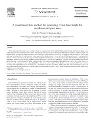
The Xixian Bas<strong>in</strong> covers an area of 10,191 km 2 and is located at <strong>the</strong> headwaters<br />
of Huaihe River, between 112 ◦ and 121 ◦ E latitude and 31 ◦ and 35 ◦ N longitude<br />
(Fig. 1). Xixian Watershed is dom<strong>in</strong>ated by mounta<strong>in</strong>s and hills, but some flat<br />
depressions cover a small part of <strong>the</strong> catchment. The watershed is situated <strong>in</strong> <strong>the</strong><br />
transition zone between <strong>the</strong> nor<strong>the</strong>rn subtropical region and <strong>the</strong> warm temperate
<strong>Evaluat<strong>in</strong>g</strong> and Compar<strong>in</strong>g <strong>the</strong> <strong>SWAT</strong> <strong>Model</strong> with <strong>the</strong> XAJ <strong>Model</strong> 2599<br />
DPL<br />
÷<br />
÷<br />
CTG<br />
÷<br />
XX<br />
§<br />
X<strong>in</strong>yang<br />
§<br />
÷<br />
ZGP<br />
Ra<strong>in</strong>-gaug<strong>in</strong>g station<br />
Y<strong>in</strong>gshan<br />
÷<br />
§<br />
Meteorological station<br />
<strong>Hydrological</strong> station<br />
Reservoir<br />
Watershed<br />
Fig. 1 Location of <strong>the</strong> Xixian Watershed and its subbas<strong>in</strong>s with hydro-meteorological stations<br />
marked<br />
zone. Mean annual precipitation is 1,145 mm and <strong>the</strong> annual average temperature<br />
is about 15.2 ◦ C. Dur<strong>in</strong>g <strong>the</strong> flood season, ra<strong>in</strong>fall is affected ma<strong>in</strong>ly by monsoons.<br />
There<strong>for</strong>e, most of <strong>the</strong> precipitation (∼50%) falls between June and September.<br />
The highest average monthly temperature is <strong>in</strong> July, and <strong>the</strong> lowest is <strong>in</strong> January.<br />
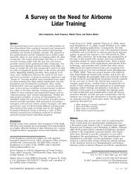
There are seven soil types <strong>in</strong> <strong>the</strong> catchment (Fig. 2b), and <strong>the</strong> top five are as follows:<br />
Shuidaotu (56%), Huanghetu (23.87%), Huangzongrangtu (9.93%), Cugutu (5.71%)<br />
and Shizhitu (3.23%%). Major land use/land cover classes are shown <strong>in</strong> Fig. 2a,<br />
<strong>in</strong>clud<strong>in</strong>g agriculture, <strong>for</strong>est and brush cover with sesbania and honey mesquite.<br />
Agriculture is <strong>the</strong> dom<strong>in</strong>ant land use, <strong>the</strong> majority of which is wheat (44.11%) and<br />
rice (16.29%) production.<br />
2.4 Input Data and <strong>Model</strong> Setup<br />
As a physically-based, distributed parameter watershed model, <strong>SWAT</strong> requires<br />
<strong>in</strong>tensive geospatial <strong>in</strong>put data to drive watershed dynamics (Table 1). The major<br />
geospatial <strong>in</strong>put data <strong>in</strong>clude, climate data, a terra<strong>in</strong> map, soil properties and a land<br />
use/land cover map. The follow<strong>in</strong>g datasets were prepared <strong>for</strong> <strong>the</strong> Xixian Watershed<br />
study: (1) a Digital Elevation <strong>Model</strong> (DEM) with a spatial resolution of 1 km<br />
(http://srtm.datamirror.csdb.cn/), (2) a year-2000 land-use map at a scale of 1:210,000<br />
(Table 2) provided by <strong>the</strong> government of X<strong>in</strong>yang city, (3) a soil map at a scale of<br />
1:100,000 <strong>in</strong> which <strong>the</strong> physical soil layer properties (<strong>in</strong>clud<strong>in</strong>g texture, bulk density,<br />
available water capacity, saturated conductivity, soil albedo and organic carbon)<br />
were collected ma<strong>in</strong>ly from Henan Soil Handbook and field observations, (4) daily<br />
climate data provided by from X<strong>in</strong>yang and Y<strong>in</strong>gshan wea<strong>the</strong>r stations (maximum<br />
and m<strong>in</strong>imum air temperature, w<strong>in</strong>d speed, solar radiation and relative humidity)<br />
and 67 ra<strong>in</strong> gauges (precipitation).
2600 P. Shi et al.<br />
a<br />
<strong>SWAT</strong> Land Cover<br />
AGRC<br />
FRST<br />
MESQ<br />
ORCD<br />
RICE<br />
RNGB<br />
RNGE<br />
SESB<br />
SWRN<br />
URHD<br />
WATR<br />
b<br />
Soil Class<br />
Cugutu<br />
Hongniantu<br />
Huanghetu<br />
Huangzongran<br />
Huichaotu<br />
Shajiangheitu<br />
Shizhit<br />
Shuidaotu<br />
Fig. 2 a Land cover and b soil maps <strong>in</strong> Xixian Bas<strong>in</strong><br />
In <strong>the</strong> del<strong>in</strong>eation of subbas<strong>in</strong>s with<strong>in</strong> <strong>the</strong> Xixian Watershed, <strong>the</strong> locations of<br />
stream stations and reservoirs were considered. Nanwan Resevoir and Shishankou<br />
Resevoir) have control areas of 1,090 and 327 km 2 , respectively. These two reservoirs<br />
and four stream stations, Dapol<strong>in</strong>g (DPL), Changtaiguan (CTG), Zhuganpu (ZGP)
<strong>Evaluat<strong>in</strong>g</strong> and Compar<strong>in</strong>g <strong>the</strong> <strong>SWAT</strong> <strong>Model</strong> with <strong>the</strong> XAJ <strong>Model</strong> 2601<br />
Table 1 Basic <strong>in</strong><strong>for</strong>mation on hydro-meteorological stations <strong>in</strong> <strong>the</strong> Xixian watershed<br />
Type of station Name Latitude Longitude Elevation Data series<br />
Meteorological station X<strong>in</strong>yang 32.117 114.083 759 1951–2005<br />
Y<strong>in</strong>gshan 31.617 113.767 933 1951–2005<br />
<strong>Hydrological</strong> station Dapol<strong>in</strong>g 32.417 113.750 107 1980–2005<br />
Changtaiguan 32.317 114.067 72 1981–2005<br />
Zhuganpu 32.167 114.650 47 1988–2005<br />
Xixian 32.333 114.733 41 1980–2005<br />
and Xixian (XX)), located with<strong>in</strong> <strong>the</strong> watershed served as subbas<strong>in</strong> outlets. In addition,<br />
to characterize <strong>the</strong> spatial variability of <strong>the</strong> watershed, a total of 33 subbas<strong>in</strong>s<br />
were del<strong>in</strong>eated (Fig. 2).<br />
2.5 <strong>Model</strong> Calibration and Validation<br />
The period from January 1, 1986 to December 31, 1986 served as a warm-up<br />
period <strong>for</strong> <strong>the</strong> model, allow<strong>in</strong>g state variables to assume realistic <strong>in</strong>itial values <strong>for</strong><br />
<strong>the</strong> calibration period. Daily runoff data from January 1, 1987 to December 31,<br />
1996 were used <strong>for</strong> calibration, and <strong>the</strong> rema<strong>in</strong><strong>in</strong>g data from January 1, 1997 to<br />
December 31, 2005 were used to validate model per<strong>for</strong>mance. Dur<strong>in</strong>g <strong>the</strong> periods<br />
of calibration, 1987, 1989, 1991 and 1996 were ra<strong>in</strong>y years, <strong>the</strong> annual precipitation<br />
were 1,515, 1,261, 1,279 and 1,279 mm, separately; 1988 was drought year, <strong>the</strong> annual<br />
precipitation was 823 mm; and <strong>the</strong> rema<strong>in</strong><strong>in</strong>g years were average years, <strong>the</strong> average<br />
annual precipitation was 1,000 mm.<br />
In this study, we followed Santhi et al. (2001) and Moriasi et al. (2007) by<br />
us<strong>in</strong>g <strong>the</strong> follow<strong>in</strong>g statistical evaluation tools: percent bias (PBIAS), coefficient of<br />
determ<strong>in</strong>ation (R 2 ), and Nash-Sutcliffe efficiency (NSE). PBIAS is calculated as:<br />
(<br />
∑ T<br />
( ) / )<br />
∑<br />
T<br />
PBIAS = Qs,t − Q m,t Q m,t × 100<br />
t=1<br />
Where Q s,t is <strong>the</strong> model simulated value at time unit t. Q m,t is <strong>the</strong> observed data<br />
value at time unit t, and t = 1,2,...,T. PBIAS measures <strong>the</strong> average tendency<br />
of <strong>the</strong> simulated data to be larger or smaller than <strong>the</strong>ir observed counterparts.<br />
PBIAS values with small magnitude are preferred. Positive values <strong>in</strong>dicate model<br />
overestimation bias while negative values <strong>in</strong>dicate underestimation (Gupta et al.<br />
1999).<br />
t=1<br />
Table 2 Xixian land use<br />
classes matched with <strong>the</strong><br />
<strong>SWAT</strong> land use classes<br />
Land use class<br />
Percentage of total<br />
catchment area<br />
AGRC (Agriculture land-close-grown) 44.11<br />
FRST (Forest-mixed) 33.66<br />
RICE (Rice) 16.29<br />
SESB (Sesbania) 5.27<br />
MESQ (Honey mesquite) 0.67
2602 P. Shi et al.<br />
The <strong>for</strong>mula <strong>for</strong> calculat<strong>in</strong>g coefficient R 2 is:<br />
⎧<br />
⎨ T∑<br />
R 2 ( )( ) /[ ] T 0.5 [<br />
∑ ( ) T<br />
] 0.5<br />
⎫<br />
2<br />
∑ ( ) ⎬ 2<br />
= Qm,t − ¯Q m Qs,t − ¯Q s Qm,t − ¯Q m Qs,t − ¯Q s<br />
⎩<br />
⎭<br />
t=1<br />
t=1<br />
t=1<br />
2<br />
where ¯Q m is mean observed data value <strong>for</strong> <strong>the</strong> entire evaluation time period, ¯Q s<br />
is <strong>the</strong> mean simulated data value <strong>for</strong> <strong>the</strong> entire evaluation time period. The o<strong>the</strong>r<br />
symbols have <strong>the</strong> same mean<strong>in</strong>g def<strong>in</strong>ed above. R 2 is equal to <strong>the</strong> square of Pearson’s<br />
product-moment correlation coefficient (Legates and McCabe 1999). It represents<br />
<strong>the</strong> proportion of total variance <strong>in</strong> <strong>the</strong> observed data that can be expla<strong>in</strong>ed by <strong>the</strong><br />
model. R 2 ranges between 0.0 and 1.0. Higher values mean better per<strong>for</strong>mance.<br />
NSE is calculated as:<br />
NSE = 1.0 −<br />
/<br />
T∑ ( ) 2<br />
∑ T<br />
( ) 2<br />
Qm,t − Q s,t Qm,t − ¯Q m<br />
t=1<br />
NSE <strong>in</strong>dicates how well <strong>the</strong> plot of observed values versus simulated values fits <strong>the</strong><br />
1:1 l<strong>in</strong>e and ranges from -∞ to 1 (Nash and Sutcliffe 1970). Larger NSE values are<br />
equivalent with better model per<strong>for</strong>mance.<br />
The orig<strong>in</strong>al design objective of <strong>the</strong> <strong>SWAT</strong> model was to operate <strong>in</strong> large-scale,<br />
ungauged bas<strong>in</strong>s with little or no calibration ef<strong>for</strong>ts (Arnold et al. 1998). Several<br />
studies have demonstrated that <strong>SWAT</strong> <strong>in</strong>put parameter values can be successfully<br />
estimated without calibration <strong>in</strong> a wide variety of hydrologic systems and geographic<br />
locations us<strong>in</strong>g readily available GIS databases that have been developed based on<br />
prior knowledge (Sr<strong>in</strong>ivasan et al. 1998; Arnold et al. 1999; Zhang et al. 2008a).<br />
Sr<strong>in</strong>ivasan et al. (2010) showed that, given appropriate <strong>in</strong>put data, <strong>SWAT</strong> was able<br />
to provide a satisfactory hydrologic model<strong>in</strong>g per<strong>for</strong>mance <strong>in</strong> <strong>the</strong> Upper Mississippi<br />
River Bas<strong>in</strong> without calibration. In contrast, previous studies (e.g., Zhang et al.<br />
2008a, 2009, 2011) showed that calibrat<strong>in</strong>g <strong>SWAT</strong> us<strong>in</strong>g automatic methods may<br />
bias parameter values towards optimization objectives, lead<strong>in</strong>g to un<strong>in</strong>tended per<strong>for</strong>mance<br />
<strong>in</strong> o<strong>the</strong>r hydrologic variables that are not used <strong>for</strong> calibration. There<strong>for</strong>e,<br />
<strong>in</strong> this study, we chose a multi-site, manual calibration of <strong>SWAT</strong> parameters with<strong>in</strong><br />
a small area of <strong>the</strong> Xixian Watershed. In <strong>the</strong> XAJ model, <strong>the</strong>re are 15 parameters<br />
related to runoff generation. However, determ<strong>in</strong><strong>in</strong>g <strong>the</strong>m us<strong>in</strong>g field measurements<br />
is never<strong>the</strong>less impractical (Zhao 1992). There<strong>for</strong>e, an optimization algorithm determ<strong>in</strong>ed<br />
many parameter values by match<strong>in</strong>g simulated and observed runoff.<br />
2.6 Parameter Sensitivity Analysis <strong>for</strong> <strong>SWAT</strong><br />
A sensitivity analysis was implemented to identify sensitive parameters <strong>for</strong> model<br />
calibration. S<strong>in</strong>ce we adopted a manual calibration approach, <strong>the</strong> sensitivity analysis<br />
plays a critical role <strong>in</strong> reduc<strong>in</strong>g parameter dimension. It helped us reduce time spent<br />
<strong>in</strong> model calibrated period. The sensitivity analysis method implemented <strong>in</strong> <strong>SWAT</strong> is<br />
Lat<strong>in</strong> Hypercube One-factor-At-a-Time (LH-OAT). The details of <strong>the</strong> method can<br />
be found <strong>in</strong> <strong>SWAT</strong>2005 Advanced Workshop (Griensven 2005).<br />
The sensitivity analysis resulted <strong>in</strong> a list of parameters ranked from most to least<br />
sensitive (Table 3). Based on this rank<strong>in</strong>g, we chose <strong>the</strong> n<strong>in</strong>e most sensitive parameters<br />
(CH_K2, SURLAG, ALPHA_BF, CN2, CH_N, SOL_AWC, GWQMN and<br />
t=1
<strong>Evaluat<strong>in</strong>g</strong> and Compar<strong>in</strong>g <strong>the</strong> <strong>SWAT</strong> <strong>Model</strong> with <strong>the</strong> XAJ <strong>Model</strong> 2603<br />
Table 3 Sensitivity analysis results<br />
Rank 1 2 3 4 5 6 7 8<br />
Parameter CH_K2 SURLAG ALPHA_BF CN2 CH_N SMFMX SOL_AWC SMTMP<br />
Rank 9 10 11 12 13 14 15 16<br />
Parameter GWQMN ESCO SLOPE SOL_K SLSUBBSN TIMP SOL_Z CANMX<br />
Rank 17 18 19 20 21 22 23 24<br />
Parameter SFTMP SMFMN BIOMIX EPCO BLAI GW_DELAY SOL_ALB GW_REVAP
2604 P. Shi et al.<br />
Table 4 <strong>SWAT</strong> flow-sensitive parameters and fitted values after calibration<br />
Parameter Def<strong>in</strong>ition DPL CTG ZGP XX<br />
CH_K2 Effective hydraulic conductivity <strong>in</strong> ma<strong>in</strong> channel 1.2 1.2 1.5 1.5<br />
SURLAG Surface runoff lag coefficient 2 2 2 2<br />
ALPHA_BF Baseflow alpha factor 0.55 0.45 0.6 0.6<br />
CN2 Curve number 14% 9% 5% 5%<br />
CH_N Mann<strong>in</strong>g’s “n” value 0.035 0.035 0.035 0.035<br />
SOL_AWC Available water capacity −0.1 −0.1 −0.1 −0.1<br />
GWQMN Threshold depth of water <strong>for</strong> return flow 100 100 100 100<br />
ESCO Soil evaporation compensation factor 0.65 0.8 0.9 0.9<br />
ESCO) with<strong>in</strong> <strong>the</strong> Xixian Watershed and <strong>the</strong>n adjusted <strong>the</strong>se parameters manually.<br />
Table 3 shows that two parameters, SMFMX and SMTMP, are more sensitive than<br />
GWQMN and ESCO, but <strong>the</strong>se two parameters represent snowmelt. Due to high<br />
temperatures, snowfall and snowmelt are not important hydrologic components <strong>in</strong><br />
our research, so we ignored <strong>the</strong>se two parameters. Sensitive parameters and postcalibration<br />
fitted values are listed <strong>in</strong> Table 4.<br />
3 Results and Discussion<br />
3.1 Mean Annual Streamflow<br />
Average annual streamflow simulated by <strong>SWAT</strong> and XAJ is listed <strong>in</strong> Table 5. The<br />
relative, simulated mean annual runoff errors of both XAJ and <strong>SWAT</strong> were less than<br />
15% at all four monitor<strong>in</strong>g stations <strong>for</strong> both calibration and validation periods. The<br />
difference between observed and simulated annual runoff volumes <strong>for</strong> XAJ ranged<br />
from −1.4% (station ZGP) to 12.1% (station DPL) <strong>for</strong> <strong>the</strong> validation period. For<br />
<strong>SWAT</strong>, <strong>the</strong> relative error <strong>in</strong> <strong>the</strong> annual runoff volumes ranged from 2.3% (station<br />
CTG) to −12.3% (station DPL) <strong>for</strong> <strong>the</strong> validation period. The accuracy of both<br />
models was similar <strong>for</strong> <strong>the</strong> calibration and validation periods. In general, both <strong>SWAT</strong><br />
and XAJ can capture long-term runoff yield <strong>in</strong> <strong>the</strong> Xixian watershed.<br />
Table 5 Observed and simulated annual runoff volumes <strong>in</strong> <strong>the</strong> Xixian Watershed<br />
Subwatershed Annual runoff volume (mm year −1 ) Relative error (%)<br />
Observed <strong>SWAT</strong> XAJ <strong>SWAT</strong> XAJ<br />
Calibration period<br />
DPL 492 446 520 −9.3 5.7<br />
CTG 430 467 440 8.6 2.3<br />
ZGP 438 450 453 2.7 3.4<br />
XX 320 322 338 0.6 5.6<br />
Validation period<br />
DPL 446 391 500 −12.3 12.1<br />
CTG 384 393 373 2.3 −2.9<br />
ZGP 495 481 488 −2.8 −1.4<br />
XX 345 323 350 −6.4 1.4
<strong>Evaluat<strong>in</strong>g</strong> and Compar<strong>in</strong>g <strong>the</strong> <strong>SWAT</strong> <strong>Model</strong> with <strong>the</strong> XAJ <strong>Model</strong> 2605<br />
3.2 Daily Streamflow<br />
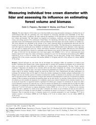
Figures 3 and 4 show <strong>SWAT</strong>-simulated time series of measured and simulated daily<br />
flow <strong>for</strong> all four river gaug<strong>in</strong>g stations dur<strong>in</strong>g calibration and validation periods.<br />
Both figures show that <strong>the</strong> observed and simulated flow discharge follows area<br />
ra<strong>in</strong>fall patterns. For example, higher discharge occurs between June and September,<br />
correspond<strong>in</strong>g to <strong>the</strong> ra<strong>in</strong>y season. Above 80% of annual flow occurs dur<strong>in</strong>g this<br />
period.<br />
Table 6 summarizes statistical per<strong>for</strong>mance measures <strong>for</strong> daily runoff volumes.<br />
Previous studies (Moriasi et al. 2007; Santhi et al. 2001) suggested that model<br />
simulation be judged as satisfactory if R 2 is greater than 0.6 and NSE is greater<br />
2000<br />
Zhuganpu<br />
0<br />
1600<br />
100<br />
flow (m3/s)<br />
flow (m3/2)<br />
1200<br />
800<br />
400<br />
0<br />
1988 1989 1990 1991 1992 1993 1994 1995 1996<br />
predicted flow measured flow ra<strong>in</strong>fall<br />
6000<br />
5000<br />
4000<br />
3000<br />
2000<br />
Xixian<br />
200<br />
300<br />
400<br />
500<br />
0<br />
100<br />
200<br />
300<br />
precipitation (mm) precipitation (mm)<br />
1000<br />
400<br />
0<br />
1987 1988 1989 1990 1991 1992 1993 1994 1995 1996<br />
predicted flow measured flow ra<strong>in</strong>fall<br />
Fig. 3 Calibration of streamflow at four gaug<strong>in</strong>g stations<br />
500
2606 P. Shi et al.<br />
4000<br />
Dapol<strong>in</strong>g<br />
0<br />
3500<br />
3000<br />
100<br />
flow (m3/s)<br />
2500<br />
2000<br />
1500<br />
200<br />
300<br />
precipitation (mm)<br />
1000<br />
500<br />
400<br />
0<br />
1987 1988 1989 1990 1991 1992 1993 1994 1995 1996<br />
predicted flow measured flow ra<strong>in</strong>fall<br />
500<br />
4000<br />
Changtaiguan<br />
0<br />
3500<br />
3000<br />
100<br />
flow (m3/s)<br />
2500<br />
2000<br />
1500<br />
200<br />
300<br />
precipitation (mm)<br />
1000<br />
500<br />
400<br />
0<br />
1987 1988 1989 1990 1991 1992 1993 1994 1995 1996<br />
predicted flow measured flow ra<strong>in</strong>fall<br />
Fig. 3 (cont<strong>in</strong>ued)<br />
500<br />
than 0.5. Comparisons between observed and simulated runoff values agreed well,<br />
<strong>in</strong>dicat<strong>in</strong>g that both <strong>SWAT</strong> and XAJ models represented observed runoff well at <strong>the</strong><br />
four gaug<strong>in</strong>g stations, DPL, CTG, ZGP and XX. For <strong>the</strong> calibration period, R 2 and<br />
NSE values obta<strong>in</strong>ed from XAJ at <strong>the</strong> four stations ranged from 0.77 to 0.87 and 0.72<br />
to 0.85, respectively. R 2 and NSE values obta<strong>in</strong>ed from <strong>SWAT</strong> were very similar,<br />
rang<strong>in</strong>g from 0.77 to 0.87 and 0.75 to 0.85, respectively. For <strong>the</strong> validation period,<br />
R 2 and NSE values obta<strong>in</strong>ed from XAJ at <strong>the</strong> four stations ranged from 0.72 to<br />
0.87 and 0.70 to 0.86, respectively. F<strong>in</strong>ally, R 2 and NSE values obta<strong>in</strong>ed from <strong>SWAT</strong><br />
ranged from 0.73 to 0.86 and 0.69 to 0.82, respectively. After <strong>the</strong> calibration of several<br />
parameters, both <strong>SWAT</strong> and XAJ models captured <strong>the</strong> study area’s hydrologic<br />
characteristics well and reproduced acceptable daily runoff simulations.
<strong>Evaluat<strong>in</strong>g</strong> and Compar<strong>in</strong>g <strong>the</strong> <strong>SWAT</strong> <strong>Model</strong> with <strong>the</strong> XAJ <strong>Model</strong> 2607<br />
2000<br />
Zhuganpu<br />
0<br />
1600<br />
100<br />
flow(m3/s)<br />
1200<br />
800<br />
200<br />
300<br />
precipitation(mm)<br />
400<br />
400<br />
0<br />
1997 1998 1999 2000 2001 2002 2003 2004 2005<br />
predicted flow measured flow ra<strong>in</strong>fall<br />
500<br />
7000<br />
Xixian<br />
0<br />
6000<br />
5000<br />
100<br />
flow(m3/s)<br />
4000<br />
3000<br />
2000<br />
1000<br />
200<br />
300<br />
400<br />
precipitation(mm)<br />
0<br />
1997 1998 1999 2000 2001 2002 2003 2004 2005<br />
predicted flow measured flow ra<strong>in</strong>fall<br />
500<br />
Fig. 4 Validation of streamflow at four gaug<strong>in</strong>g stations<br />
3.3 Runoff Components Simulated by <strong>SWAT</strong> and XAJ<br />
A reasonable representation of different runoff components is critical <strong>for</strong> captur<strong>in</strong>g<br />
<strong>the</strong> hydrologic cycle. To separate baseflow from total runoff, we used <strong>the</strong> digital<br />
baseflow filter (Arnold and Allen 1999), a program that has per<strong>for</strong>med well <strong>in</strong><br />
comparisons with measured field estimates <strong>in</strong> multiple watersheds. The results show<br />
that baseflow contributes about 48–49% of <strong>the</strong> streamflow. Table 7 shows Xixian<br />
Watershed runoff components simulated by both <strong>SWAT</strong> and XAJ. For <strong>the</strong> XAJ<br />
model, surface runoff contributes 52% and 47% to <strong>the</strong> water yield dur<strong>in</strong>g <strong>the</strong><br />
calibration and validation period respectively. Groundwater contributes 48% and<br />
53% to <strong>the</strong> water yield dur<strong>in</strong>g calibration and validation periods, respectively. For <strong>the</strong>
2608 P. Shi et al.<br />
2000<br />
Dapol<strong>in</strong>g<br />
0<br />
1600<br />
100<br />
flow(m3/s)<br />
1200<br />
800<br />
200<br />
300<br />
precipitation(mm)<br />
400<br />
400<br />
0<br />
1997 1998 1999 2000 2001 2002 2003 2004 2005<br />
predicted flow measured flow ra<strong>in</strong>fall<br />
500<br />
3500<br />
Changtaiguan<br />
0<br />
flow(m3/s)<br />
3000<br />
2500<br />
2000<br />
1500<br />
1000<br />
500<br />
100<br />
200<br />
300<br />
400<br />
precipitation(mm)<br />
0<br />
1997 1998 1999 2000 2001 2002 2003 2004 2005<br />
predicted flow measured flow ra<strong>in</strong>fall<br />
500<br />
Fig. 4 (cont<strong>in</strong>ued)<br />
<strong>SWAT</strong> model, results <strong>in</strong>dicate that surface runoff contributions dur<strong>in</strong>g calibration<br />
and validation periods are 53% and 56%, respectively, and groundwater contributes<br />
47% and 44% to <strong>the</strong> water yield <strong>for</strong> calibration and validation periods, respectively.<br />
Overall, both <strong>SWAT</strong> and XAJ provide reasonable surface runoff and baseflow<br />
contributions, <strong>in</strong>dicat<strong>in</strong>g <strong>the</strong>ir ability to represent <strong>the</strong> hydrologic cycle well.<br />
3.4 Comparison of <strong>Model</strong> Structure and Functions <strong>in</strong> <strong>SWAT</strong> and XAJ<br />
As <strong>in</strong>dicated <strong>in</strong> previous sections, <strong>SWAT</strong> and XAJ per<strong>for</strong>m similarly <strong>in</strong> runoff<br />
simulations. In order to provide <strong>in</strong>sight <strong>in</strong>to <strong>the</strong> suitability of each model <strong>for</strong>
<strong>Evaluat<strong>in</strong>g</strong> and Compar<strong>in</strong>g <strong>the</strong> <strong>SWAT</strong> <strong>Model</strong> with <strong>the</strong> XAJ <strong>Model</strong> 2609<br />
Table 6 Statistical comparison of observed and simulated daily runoff <strong>for</strong> <strong>the</strong> Xixian Watershed<br />
Subwatershed PBIAS (%) R 2 NSE<br />
XAJ <strong>SWAT</strong> XAJ <strong>SWAT</strong> XAJ <strong>SWAT</strong><br />
Calibration period<br />
DPL 5.53 −9.32 0.87 0.84 0.85 0.84<br />
CTG 2.46 −14.8 0.86 0.87 0.79 0.85<br />
ZGP 5.04 −1.30 0.77 0.81 0.73 0.79<br />
XX 5.58 1.75 0.78 0.77 0.72 0.75<br />
Validation period<br />
DPL 8.2 −12.3 0.87 0.82 0.86 0.82<br />
CTG −2.93 −3.9 0.74 0.86 0.72 0.79<br />
ZGP −1.52 −13.0 0.76 0.78 0.71 0.76<br />
XX 1.31 −6.41 0.72 0.73 0.70 0.69<br />
susta<strong>in</strong>able water resource management <strong>in</strong> <strong>the</strong> Xixian Watershed, Table 8 provides<br />
a comprehensive comparison of <strong>the</strong> models’ characteristics.<br />
Concern<strong>in</strong>g model structure, XAJ is a traditional, conceptual, lumped hydrologic<br />
model with simple structure. In contrast, <strong>SWAT</strong> is a distributed hydrologic model<br />
with a relatively complicated process-based model structure. Both of <strong>the</strong>se two<br />
models are widely used. XAJ is typically used <strong>for</strong> <strong>for</strong>ecast<strong>in</strong>g flood and runoff over<br />
a catchment scale. On <strong>the</strong> o<strong>the</strong>r hand, <strong>SWAT</strong> divides a watershed <strong>in</strong>to multiple<br />
subbas<strong>in</strong>s, which are <strong>the</strong>n fur<strong>the</strong>r subdivided <strong>in</strong>to HRUs to represent <strong>the</strong> heterogeneity<br />
of land use, management and soil characteristics. In XAJ, <strong>the</strong> catchment was<br />
represented as homogeneous. Human activities (e.g., urban, reservoir, agricultural<br />
activity, etc.) cannot be reflected directly <strong>in</strong> XAJ. To some extent, this limitation<br />
restricts <strong>the</strong> application doma<strong>in</strong> of XAJ to water quantity model<strong>in</strong>g only. Many<br />
human activities (e.g., <strong>in</strong>dustry discharge and fertilizer application on crop land)<br />
impact water quality and can be directly <strong>in</strong>put and simulated <strong>in</strong> <strong>the</strong> <strong>SWAT</strong> model.<br />
It is also worth not<strong>in</strong>g that, <strong>in</strong> order to successfully apply <strong>the</strong>se two models,<br />
<strong>in</strong>put data preparation ef<strong>for</strong>ts are substantially different. The <strong>in</strong>put data required by<br />
XAJ is relatively simple, <strong>in</strong>clud<strong>in</strong>g only areal mean precipitation and measured pan<br />
evaporation. However, <strong>in</strong>tensive data collection and process<strong>in</strong>g work are required<br />
to run <strong>the</strong> <strong>SWAT</strong> model. DEM, land use, soil type and human activity data must<br />
be provided. Although <strong>SWAT</strong>’s GIS <strong>in</strong>terface can reduce data preparation ef<strong>for</strong>ts,<br />
it takes much longer to run <strong>SWAT</strong> than XAJ. There<strong>for</strong>e, <strong>for</strong> flood <strong>for</strong>ecast<strong>in</strong>g<br />
and runoff simulation, XAJ is a preferred tool. In order to ma<strong>in</strong>ta<strong>in</strong> water susta<strong>in</strong>-<br />
Table 7 Annual water balance components <strong>for</strong> calibration and validation periods <strong>in</strong> <strong>the</strong> Xixian Bas<strong>in</strong><br />
(mm)<br />
Period <strong>Model</strong> Surface Ground Total Baseflow Baseflow<br />
flow flow flow ratio separation<br />
Calibration XAJ 176 162 338 0.48 0.48<br />
<strong>SWAT</strong> 172 150 322 0.47<br />
Validation XAJ 163 187 350 0.53 0.49<br />
<strong>SWAT</strong> 182 141 323 0.44
2610 P. Shi et al.<br />
Table 8 Comparison of <strong>SWAT</strong> and XAJ<br />
<strong>SWAT</strong><br />
<strong>Model</strong> Structure Processed-based Conceptual<br />
Spatial scale HRU with<strong>in</strong> subbas<strong>in</strong> Subbas<strong>in</strong><br />
Temporal scale Hourly and daily Hourly an daily<br />
Input data requirements Intensive data collection on Climate <strong>in</strong>puts and<br />
climate, soil, topography, land use, topography<br />
vegetation, hydrologic structures<br />
and human activities.<br />
Extendibility <strong>for</strong> water Includes sediment, nitrogen, phosphorus, No water quality model<strong>in</strong>g<br />
quality model<strong>in</strong>g bacteria, heavy metals,and pesticides functions<br />
Interface User friendly GIS <strong>in</strong>terface <strong>for</strong> No GIS <strong>in</strong>terface available<br />
preprocess<strong>in</strong>g and preprocess<strong>in</strong>g<br />
XAJ<br />
ability, two <strong>in</strong>herent two dimensions—quantity and quality—should be emphasized<br />
simultaneously. <strong>SWAT</strong>’s strong po<strong>in</strong>t is that it can simultaneously simulate water<br />
quantity and quality and evaluate <strong>the</strong> impacts of human activities on susta<strong>in</strong>able<br />
water resource management <strong>in</strong> <strong>the</strong> Xixian Watershed.<br />
4 Conclusion<br />
This research compared <strong>the</strong> runoff simulation per<strong>for</strong>mance of two widely used hydrologic<br />
models <strong>in</strong> <strong>the</strong> Xixian Watershed, located <strong>in</strong> <strong>the</strong> upper reaches of <strong>the</strong> Huaihe<br />
River Bas<strong>in</strong>. The results show that <strong>SWAT</strong> and XAJ per<strong>for</strong>m equally and both can<br />
simulate daily runoff satisfactorily. Compar<strong>in</strong>g simulated and observed daily flow<br />
at four monitor<strong>in</strong>g stations, both models produced R 2 and NSE values larger than<br />
0.69 and PBIAS values lower than 15% <strong>for</strong> both calibration and validation periods.<br />
These two models can also simulate runoff components well <strong>in</strong> comparison to <strong>the</strong><br />
results from <strong>the</strong> baseflow filter.<br />
The XAJ model is easy to use with m<strong>in</strong>imum <strong>in</strong>put data preparation. In order<br />
to run <strong>SWAT</strong>, many data-preparation ef<strong>for</strong>s must be made. For <strong>the</strong> purposes of<br />
flood <strong>for</strong>ecast<strong>in</strong>g and runoff simulation, XAJ is preferred. However, <strong>the</strong> complex,<br />
processes-based <strong>SWAT</strong> model can simultaneously simulate water quantity and<br />
quality and evaluate <strong>the</strong> impacts of land use changes and human activities. This<br />
makes <strong>SWAT</strong> a better tool <strong>for</strong> susta<strong>in</strong>able water resources management <strong>in</strong> <strong>the</strong> Xixian<br />
Watershed, where agricultural activities are <strong>in</strong>tensive.<br />
Acknowledgements The first author thanks <strong>the</strong> follow<strong>in</strong>g f<strong>in</strong>ancial support: <strong>the</strong> Special Fund<br />
of State Key Laboratory of Ch<strong>in</strong>a (2009586412); <strong>the</strong> Ph.D. Programs Foundation of M<strong>in</strong>istry of<br />
Education, Ch<strong>in</strong>a (20090094120008); <strong>the</strong> Fundamental Research Funds <strong>for</strong> <strong>the</strong> Central Universities;<br />
<strong>the</strong> National Natural Science Foundation of Ch<strong>in</strong>a (No. 41001011/40901015/51079038); <strong>the</strong> Commonweal<br />
Project Granted by <strong>the</strong> M<strong>in</strong>istry of Water Resources of <strong>the</strong> People’s Republic of Ch<strong>in</strong>a<br />
(No. 200701031); <strong>the</strong> National Natural Science Foundation of Ch<strong>in</strong>a (No. 40930635); <strong>the</strong> Program<br />
<strong>for</strong> Changjiang Scholars and Innovative Research Team <strong>in</strong> University (IRT0717) and <strong>the</strong> Ground<br />
Project Granted by <strong>the</strong> M<strong>in</strong>istry of Education of <strong>the</strong> People’s Republic of Ch<strong>in</strong>a (20064).
<strong>Evaluat<strong>in</strong>g</strong> and Compar<strong>in</strong>g <strong>the</strong> <strong>SWAT</strong> <strong>Model</strong> with <strong>the</strong> XAJ <strong>Model</strong> 2611<br />
References<br />
Abbott MB, Bathurst JC, Cunge JA, O’Connell PE, Rasmussen J (1986) An <strong>in</strong>troduction to <strong>the</strong><br />
European hydrological system-systeme hydrologique European ‘SHE’. 1: history and philosophy<br />
of a physically based distributed model<strong>in</strong>g system. J Hydrol 87:45–59<br />
Arnold JG, Allen PM (1999) Automated methods <strong>for</strong> estimat<strong>in</strong>g baseflow and ground water<br />
recharge from streamflow records. J Am Water Resour Assoc 35(2):411–424<br />
Arnold JG, Williams JR, Sr<strong>in</strong>ivasan R, K<strong>in</strong>g KW (1996) In soil and water assessment tool, user’s<br />
manual. USDA, Agriculture Research Service, Grassland, Soil and Water Research Laboratory,<br />
Temple<br />
Arnold JG, Sr<strong>in</strong>ivasan R, Muttiah RS, Williams JR (1998) Large area hydrologic model<strong>in</strong>g and<br />
assessment part I: model development. J Am Water Resour Assoc 34(1):73–89<br />
Arnold JG, Sr<strong>in</strong>ivasan R, Ramanarayanan TS, DiLuzio M (1999) Water resources of <strong>the</strong> Texas Gulf<br />
Bas<strong>in</strong>. Water Sci Technol 39(3):121–133<br />
Beasley DB, Hygg<strong>in</strong>s LF (1995) ANSWERS-User’s Manual. U.S. Environmental Protection Agency,<br />
Chicago, EPA-905/9-82-001, p54<br />
Cao W, Bowden WB, Davie T, Fenemor A (2009) <strong>Model</strong>l<strong>in</strong>g impacts of land cover change on<br />
critical water resources <strong>in</strong> <strong>the</strong> Motueka River catchment, New Zealand. Water Resour Manag<br />
23:137–151<br />
Debele B, Sr<strong>in</strong>ivasan R, Gosa<strong>in</strong> AK (2010) Comparsion of Process-Based and Temperature-Index<br />
Snowmelt <strong>Model</strong><strong>in</strong>g <strong>in</strong> <strong>SWAT</strong>. Water Resour Manag 24:1065–1088<br />
Griensven AV (2005) AV<strong>SWAT</strong>-X <strong>SWAT</strong>-2005 Advanced Workshop. In: <strong>SWAT</strong> 2005 3rd International<br />
Conference, Zurich, Switzerland<br />
Gupta HV, Sorooshian S, Yapo PO (1999) Status of automatic calibration <strong>for</strong> hydrologic models:<br />
Comparison with multilevel expert calibration. J Hydrol Eng 4(2):135–143<br />
Holvoet K, Gevaert V, Griensver AV, Seuntjens P, Vanrolleghem PA (2007) <strong>Model</strong>l<strong>in</strong>g <strong>the</strong><br />
effectiveness of agricultural measures to reduce <strong>the</strong> amount of pesticides enter<strong>in</strong>g surface waters.<br />
Water Resour Manag 21:2027–2035<br />
Johansen NB, Imhoff JC, Kittle JL, Donigian AS (1984) <strong>Hydrological</strong> Simulation Program-Fortran<br />
(HSPF): User’s Manual <strong>for</strong> Release 8. US Environmental Protection Agency, A<strong>the</strong>ns, EPA-<br />
600/3-84-066<br />
Legates DR, McCabe GJ (1999) <strong>Evaluat<strong>in</strong>g</strong> <strong>the</strong> use of “goodness of fit” measures <strong>in</strong> hydrologic and<br />
hydroclimatic model validation. Water Resour Res 35(1):233–241<br />
Moriasi DN, Arnold JG, Van Liew MU, B<strong>in</strong>ger RL, Harmel RD, Veith T (2007) <strong>Model</strong> evaluation<br />
guidel<strong>in</strong>es <strong>for</strong> systematic quantification of accuracy <strong>in</strong> watershed simulations. Trans ASABE<br />
50(3):885–900<br />
Nash JE, Sutcliffe JC (1970) River flow <strong>for</strong>ecast<strong>in</strong>g through conceptual models. Part I—A discussion<br />
of pr<strong>in</strong>ciples. J Hydrol 10:282–290<br />
Neitsch SL, Arnold JG, K<strong>in</strong>iry JR, Williams JR (2005a) <strong>SWAT</strong> <strong>the</strong>oretical documentation version<br />
2005. Grassland, Soil and Water Research Laboratory, Agricultural Research Service, Temple<br />
Neitsch SL, Arnold JG, K<strong>in</strong>iry JR, Williams JR (2005b) <strong>SWAT</strong> <strong>in</strong>put/output file documentation<br />
version 2005. Grassland, Soil and Water Research Laboratory, Agricultural Research Service,<br />
Temple<br />
Santhi C, Arnold JG, Williams JR, Dugas WA, Sr<strong>in</strong>ivasn R, Hauck LM (2001) Validation of <strong>the</strong><br />
<strong>SWAT</strong> model on a large river bas<strong>in</strong> with po<strong>in</strong>t and nonpo<strong>in</strong>t sources. J Am Water Resour Assoc<br />
37(5):1169–1188<br />
Shi P, Rui X, Qu S (2008) Calculat<strong>in</strong>g storage capacity with topographic <strong>in</strong>dex. Advances <strong>in</strong> Water<br />
Sci 19(2):264–267 (<strong>in</strong> Ch<strong>in</strong>ese)<br />
Sr<strong>in</strong>ivasan R, Ramanarayanan TS, Arnold JG, Bednarz ST (1998) Large area hydrologic model<strong>in</strong>g<br />
and assessment part II: model application. J Am Water Resour Assoc 34(1):91–101<br />
Sr<strong>in</strong>ivasan R, Zhang X, Arnold JG (2010) <strong>SWAT</strong> Ungauged: hydrologic and Biofuel Crops Prediction<br />
<strong>in</strong> <strong>the</strong> Upper Mississippi River Bas<strong>in</strong>. Trans ASABE 53(5):1533–1546<br />
Van Liew MW, Garbrecht JD (2003) Hydrologic simulation of <strong>the</strong> Little Washita River Experiment<br />
Watershed us<strong>in</strong>g <strong>SWAT</strong>. J Am Water Resour Assoc 39(2):413–426<br />
Van Liew MW, Veith TL, Bosch DD, Arnold JG (2007) Suitability of <strong>SWAT</strong> <strong>for</strong> <strong>the</strong> conservation<br />
effects assessment project: comparison on USDA agricultural research service Watersheds. J<br />
Hydrol Eng 12(2):173–189<br />
Young RA, Onstad CA, Bosch DD, Anderson WP (1987) AGNPS: an agricultural nonpo<strong>in</strong>t source<br />
pollution model: a large watershed analysis tool. Conservation Research Report 35. US Department<br />
of Agriculture, Wash<strong>in</strong>gton, DC, p77
2612 P. Shi et al.<br />
Zhang X, Sr<strong>in</strong>ivasan R, Debele B, Hao F (2008a) Runoff Simulation of <strong>the</strong> Headwaters of <strong>the</strong><br />
Yellow River Us<strong>in</strong>g <strong>the</strong> Swat <strong>Model</strong> with Three Snowmelt Algorithms. J Am Water Resour<br />
Assoc 44(1):48–61<br />
Zhang X, Sr<strong>in</strong>ivasan R, Van Liew M (2008b) Multi-Site Calibration of <strong>the</strong> <strong>SWAT</strong> <strong>Model</strong> <strong>for</strong> Hydrologic<br />
<strong>Model</strong><strong>in</strong>g. Trans ASABE 51(6):2039–2049<br />
Zhang X, Sr<strong>in</strong>ivasan R, Bosch D (2009) Calibration and uncerta<strong>in</strong>ty analysis of <strong>the</strong> <strong>SWAT</strong> model<br />
us<strong>in</strong>g Genetic Algorithms and Bayesian <strong>Model</strong> Averag<strong>in</strong>g. J Hydrol 374(3–4):307–317<br />
Zhang Y, Jun X, Tao L, Quanxi S (2010) Impact of water projects on river flow regimes and water<br />
quality <strong>in</strong> Huai River bas<strong>in</strong>. Water Resour Manag 24:889–908<br />
Zhang X, Sr<strong>in</strong>ivasan R, Arnold J, Izaurralde RC, Bosch D (2011) Simultaneous calibration of surface<br />
flow and baseflow simulations: a revisit of <strong>the</strong> <strong>SWAT</strong> model calibration framework. Hydrol<br />
Process 25. doi:10.1002/hyp.8058<br />
Zhao RJ (1992) X<strong>in</strong>anjiang model applied <strong>in</strong> Ch<strong>in</strong>a. J Hydrol 135(2):371–381<br />
Zhao RJ, Zuang Y, Fang L, Liu X, Zhang Q (1980) The X<strong>in</strong>anjiang <strong>Model</strong>. IAHS AISH Publ<br />
129:351–356<br />
Zhao RJ (1993) A non-l<strong>in</strong>ear system <strong>for</strong> bas<strong>in</strong> concentration. J Hydrol 142(7):477–482