Linear interpolation of histograms

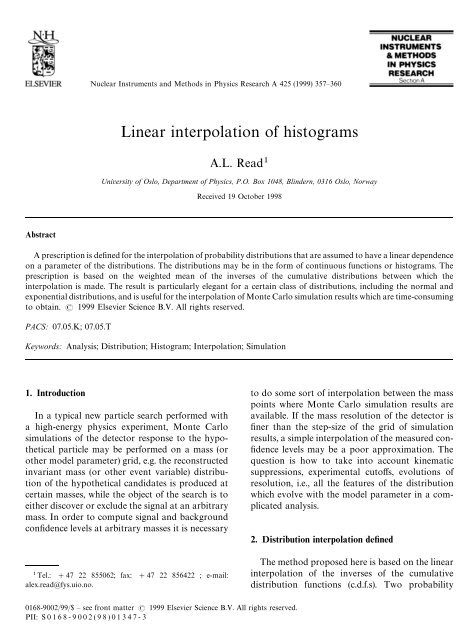
Nuclear Instruments and Methods in Physics Research A 425 (1999) 357—360
Linear interpolation of histograms
A.L. Read
University of Oslo, Department of Physics, P.O. Box 1048, Blindern, 0316 Oslo, Norway
Received 19 October 1998
Abstract
A prescription is defined for the interpolation of probability distributions that are assumed to have a linear dependence
on a parameter of the distributions. The distributions may be in the form of continuous functions or histograms. The
prescription is based on the weighted mean of the inverses of the cumulative distributions between which the
interpolation is made. The result is particularly elegant for a certain class of distributions, including the normal and
exponential distributions, and is useful for the interpolation of Monte Carlo simulation results which are time-consuming
to obtain. 1999 Elsevier Science B.V. All rights reserved.
PACS: 07.05.K; 07.05.T
Keywords: Analysis; Distribution; Histogram; Interpolation; Simulation
1. Introduction
In a typical new particle search performed with
a high-energy physics experiment, Monte Carlo
simulations of the detector response to the hypothetical
particle may be performed on a mass (or
other model parameter) grid, e.g. the reconstructed
invariant mass (or other event variable) distribution
of the hypothetical candidates is produced at
certain masses, while the object of the search is to
either discover or exclude the signal at an arbitrary
mass. In order to compute signal and background
confidence levels at arbitrary masses it is necessary
Tel.: #47 22 855062; fax: #47 22 856422 ; e-mail:
alex.read@fys.uio.no.
to do some sort of interpolation between the mass
points where Monte Carlo simulation results are
available. If the mass resolution of the detector is
finer than the step-size of the grid of simulation
results, a simple interpolation of the measured confidence
levels may be a poor approximation. The
question is how to take into account kinematic
suppressions, experimental cutoffs, evolutions of
resolution, i.e., all the features of the distribution
which evolve with the model parameter in a complicated
analysis.
2. Distribution interpolation defined
The method proposed here is based on the linear
interpolation of the inverses of the cumulative
distribution functions (c.d.f.s). Two probability
0168-9002/99/$ — see front matter 1999 Elsevier Science B.V. All rights reserved.
PII: S 0 1 6 8 - 9 0 0 2 ( 9 8 ) 0 1 3 4 7 - 3

358 A.L. Read / Nuclear Instruments and Methods in Physics Research A 425 (1999) 357—360
distribution functions (p.d.f.s) for the observable x, 3. Interpolating distributions of the form g((xx o )/k)
fM (x)" f (x ) f (x )
af (x )#bf (x ) . (8) fM (x)"g x!xN
kM
. (18)
f (x) and f (x) (defined in the physical region
x5!R), have corresponding c.d.f.s
The prescription for linear interpolation of p.d.f.s
defined in Eqs. (4)—(6) takes a particularly elegant
F (x)" (x)dx, (1)
form when the initial p.d.f.s can both be described
by the same function with different arguments of
f
F (x)" a particular form. Suppose that
(x)dx. (2)
f
f (x)"g
The goal is to obtain a new p.d.f. fM (x) with its
k
, (9)
corresponding c.d.f.
f (x)"g
FM (x)"
fM
k
, (10)
(x)dx (3)
G
that describe the new distribution. The first step of
k
" g
dx, (11)
k
the interpolation procedure is to find x and where x and k regulate the offset and scale features
of p.d.f. i. Eq. (4) takes the form
x where the cumulative distributions F and
F are equal for a given cumulative probability y,
G
F (x )"F (x )"y. (4)
!x
k
"G x !x "y. (12)
k
The cumulative probability for the new distribution
FM is set to the same value y at a linearly interpolated
This implies that the arguments in Eq. (12) have the
same value λ,
position x,
FM (x)"y, (5)
λ" x !x " !x . k k
(13)
x"ax #bx .
(6) Substitution of these results in Eq. (5) yields
The constants a and b express the interpolation FM (x)"G(λ), (14)
distance between the extreme values of the relevant
parameter for the two existing distributions (and by
construction satisfy a#b"1). For a new particle
search, for instance, this could be the relative position
i.e. the same function describes both the initial and
the interpolated cumulative distributions. Substitution
in Eq. (6) yields
of the mass hypothesis between two masses for
which the observable invariant mass distributions λ" x!x , have been computed in a Monte Carlo simulation.
kM
(15)
The p.d.f. fM (x) is obtained by inverting the cumulative
distributions in Eqs. (4) and (5), substituting
these results in Eq. (6),
where
xN
"ax #bx , (16)
FM (y)"aF
(y)#bF (y),
(7) kM "ak #bk .
(17)
deriving this with respect to y and solving for the
interpolated p.d.f. fM (x),
The interpolated p.d.f. fM (x) is then obtained by
derivation of G(λ),

A.L. Read / Nuclear Instruments and Methods in Physics Research A 425 (1999) 357—360 359
Fig. 1. Example of histogram interpolation. The reconstructed invariant mass distribution for a 60 GeV/c Higgs (solid line) has been
obtained by interpolation between the simulation results for 50 (dotted line) and 70 (dash-dotted line) GeV/c Higgs masses and is
overlaid with the simulation results of a 60 GeV/c Higgs (dashed line).
This means, for instance, that if both initial p.d.f.s
are normal distributions, the interpolated distribution
is also a normal distribution with both
the variance and mean linearly interpolated
between those of the initial distributions. For
exponential decay distributions (x
"0,k(0)
the decay constant of the interpolated distribution
is linearly interpolated between the decay constants
of the initial distributions. The same elegant
result is also obtained whenever both initial
distributions can be described by the same
power series in (x!x
)/k
.
between the 3 mass distributions (these distributions
were chosen to illustrate the interpolation
precisely because they have several, rapidly evolving
features which could be difficult to interpolate).
Since the interpolation is able to predict so well the
main features of the 60 GeV/c simulation results, it
is plausible that the smaller interpolation distances
(42.5 GeV/c) used in the DELPHI Higgs search
will lead to results superior to those obtained by
more simple means (for example simply using the
nearest available distribution or shifting it by
the difference between the mass hypothesis and the
simulated mass).
4. Interpolation of histograms
For a pair of initial distributions obtained by
histogramming the output of a complex physics
and detector simulation, it may not be practical to
identify a particular function which can describe
both initial distributions, but it is always possible
to carry out the computation in Eqs. (4)—(8)
on the histograms directly in order to obtain an
interpolated histogram. Fig. 1 shows how well the
interpolation procedure manages to describe the
reconstructed invariant mass distribution of a
hypothetical Standard Model Higgs boson with
mass m
"60 GeV/c decaying in the
ZHPeeH channel at center-of-mass energy
s"161 GeV based on simulations at m
" 50
and 70 GeV/c [1], despite the large differences
5. Conclusion
A method for linearly interpolating probability
distribution functions or histograms has been presented
here. The method gives particularly intuitive
results for certain well-known probability distribution
functions, such as the normal distribution,
where the mean and variance parameters are simply
linearly interpolated between those of the initial
pair of distributions. The method can also be applied
to histogrammed simulation data where the
distribution functions are not known and are very
different from each other, and surprisingly reasonable
results may be obtained.

360 A.L. Read / Nuclear Instruments and Methods in Physics Research A 425 (1999) 357—360
Acknowledgements
This work was supported by a grant from the
Norwegian Research Council. I would like to thank
my DELPHI colleagues for permission to use their
published Higgs search simulation results to illustrate
the histogram interpolation.
References
[1] DELPHI Collaboration, Search for neutral and charged
Higgs bosons in ee collisions at s"161 GeV and
172 GeV, Eur. Phys. J. C 2 (1998) 1.