LECTURES ON PSEUDO-HOLOMORPHIC CURVES AND THE ...
LECTURES ON PSEUDO-HOLOMORPHIC CURVES AND THE ...
LECTURES ON PSEUDO-HOLOMORPHIC CURVES AND THE ...

Create successful ePaper yourself
Turn your PDF publications into a flip-book with our unique Google optimized e-Paper software.
<strong>LECTURES</strong> <strong>ON</strong> <strong>PSEUDO</strong>-<strong>HOLOMORPHIC</strong> <strong>CURVES</strong> <strong>AND</strong> <strong>THE</strong><br />
SYMPLECTIC ISOTOPY PROBLEM<br />
BERND SIEBERT <strong>AND</strong> GANG TIAN<br />
Abstract. The purpose of these notes is a more self-contained presentation of<br />
the results of the authors in [SiTi3]. Some applications are also given.<br />
Contents<br />
Introduction 2<br />
1. Pseudo-holomorphic curves 3<br />
1.1. Almost complex and symplectic geometry 3<br />
1.2. Basic properties of pseudo-holomorphic curves 4<br />
1.3. Moduli spaces 5<br />
1.4. Applications 8<br />
1.5. Pseudo-analytic inequalities 10<br />
2. Unobstructedness I: Smooth and nodal curves 12<br />
2.1. Preliminaries on the ¯ ∂-equation 12<br />
2.2. The normal ¯ ∂-operator 13<br />
2.3. Immersed curves 16<br />
2.4. Smoothings of nodal curves 17<br />
3. The theorem of Micallef and White 18<br />
3.1. Statement of theorem 18<br />
3.2. The case of tacnodes 18<br />
3.3. The general case 20<br />
4. Unobstructedness II: The integrable case 20<br />
4.1. Motivation 20<br />
4.2. Special covers 21<br />
4.3. Description of deformation space 23<br />
4.4. The holomorphic normal sheaf 24<br />
4.5. Computation of the linearization 27<br />
4.6. A vanishing theorem 28<br />
4.7. The unobstructedness theorem 28<br />
5. Application to symplectic topology in dimension four 29<br />
5.1. Monodromy representations — Hurwitz equivalence 30<br />
5.2. Hyperelliptic Lefschetz fibrations. 31<br />
5.3. Braid Monodromy and the structure of hyperelliptic Lefschetz<br />
fibrations. 33<br />
5.4. Symplectic Noether-Horikawa surfaces. Conjectures 35<br />
6. The C 0 -compactness theorem for pseudo-holomorphic curves 37<br />
Date: December 11, 2005.<br />
1
2 BERND SIEBERT <strong>AND</strong> GANG TIAN<br />
6.1. Statement of theorem. Conventions. 37<br />
6.2. The monotonicity formula for pseudo-holomorphic maps. 38<br />
6.3. A removable singularities theorem. 40<br />
6.4. Proof of theorem. 41<br />
7. Second variation of the ¯ ∂J-equation and applications 45<br />
7.1. Comparisons of first and second variations 45<br />
7.2. Moduli spaces of pseudo-holomorphic curves with prescribed<br />
singularities 47<br />
7.3. The locus of constant deficiency 48<br />
7.4. Second variation at ordinary cusps 51<br />
8. The isotopy theorem 54<br />
8.1. Statement of theorem and discussion 54<br />
8.2. Pseudo-holomorphic techniques for the isotopy problem 55<br />
8.3. The Isotopy Lemma 56<br />
8.4. Sketch of proof 58<br />
References 61<br />
Introduction<br />
This text is an expanded version of the lectures delivered by the authors at the CIME<br />
summer school ”Symplectic 4-manifolds and algebraic surfaces”, Cetraro (Italy),<br />
September 2–10, 2003. The aim of these lectures were mostly to introduce graduate<br />
students to pseudo-holomorphic techniques for the study of the problem of isotopy<br />
of symplectic submanifolds in dimension four. We tried to keep the style of the<br />
lectures by emphasizing the basic reasons for the correctness of a result rather than<br />
by providing full details.<br />
Essentially none of the content claims any originality, but most of the results are<br />
scattered in the literature in sometimes hard-to-read locations. For example, we<br />
give a hands-on proof of the smooth parametrization of the space of holomorphic<br />
cycles on a complex surface under some positivity assumption. This is usually<br />
derived by the big machinery of deformation theory together with Banach-analytic<br />
methods. For an uninitiated person it is hard not only to follow the formal arguments<br />
needed to deduce the result from places in the literature, but also, and maybe<br />
more importantly, to understand why it is true. While our treatment here has<br />
the disadvantage to consider only a particular situation that does not even quite<br />
suffice for the proof of the Main Theorem (Theorem 8.1) we hope that it is useful<br />
for enhancing the understanding of this result outside the community of hardcore<br />
complex analysts and abstract algebraic geometers.<br />
One lecture was devoted to the beautiful theorem of Micallef and White on the<br />
holomorphic nature of pseudo-holomorphic curve singularities. The original paper is<br />
quite well written and this might be the reason that a proof of this theorem has not<br />
appeared anywhere else until very recently, in the excellent monograph [McSa3]. It<br />
devotes an appendix of 40 pages length to a careful derivation of this theorem and<br />
of most of the necessary analytical tools. Following the general principle of these<br />
lecture notes our purpose here is not to give a complete and necessarily technical<br />
proof, but to condense the original proof to the essentials. We tried to achieve
SYMPLECTIC ISOTOPY 3<br />
this goal by specializing to the paradigmical case of tacnodal singularities with a<br />
“half-integrable” complex structure.<br />
Another section treats the compactness theorem for pseudo-holomorphic curves.<br />
A special feature of the presented proof is that it works for sequences of almost<br />
complex structures only converging in the C 0 -topology. This is essential in the<br />
application to the symplectic isotopy problem.<br />
We also give a self-contained presentation of Shevchishin’s study of moduli spaces<br />
of equisingular pseudo-holomorphic maps and of second variations of pseudo-holomorphic<br />
curves. Here we provide streamlined proofs of the two results from [Sh] that<br />
we use by only computing the second variation in the directions actually needed for<br />
our purposes.<br />
The last section discusses the proof of the main theorem, which is also the main<br />
result from [SiTi3]. The logic of this proof is a bit involved, involving several reduction<br />
steps and two inductions, and we are not sure if the current presentation really<br />
helps in understanding what is going on. Maybe somebody else has to take this up<br />
again and add new ideas into streamlining this bit!<br />
Finally there is one section on the application to symplectic Lefschetz fibrations.<br />
This makes the link to the other lectures of the summer school, notably to those by<br />
Auroux and Smith.<br />
1. Pseudo-holomorphic curves<br />
1.1. Almost complex and symplectic geometry. An almost complex structure<br />
on a manifold M is a bundle endomorphism J : TM → TM with square − idTM . In<br />
other words, J makes TM into a complex vector bundle and we have the canonical<br />
decomposition<br />
TM ⊗R C = T 1,0 0,1<br />
M ⊕ TM = TM ⊕ TM<br />
into real and imaginary parts. The second equality is an isomorphism of complex<br />
vector bundles and TM is just another copy of TM with complex structure −J. For<br />
switching between complex and real notation it is important to write down the latter<br />
identifications explicitly:<br />
TM −→ T 1,0<br />
M<br />
� �<br />
1 , X ↦−→ X − iJX ,<br />
and similarly with X+iJX for T 0,1<br />
M . Standard examples are complex manifolds with<br />
J(∂xµ) = ∂yµ, J(∂yµ) = −∂xµ for holomorphic coordinates zµ = xµ + iyµ. Then the<br />
above isomorphism sends ∂xµ,∂yµ ∈ TM to ∂zµ,i∂zµ ∈ T 1,0<br />
M and to ∂¯zµ,i∂¯zµ ∈ T 0,1<br />
M<br />
respectively. Such integrable almost complex structures are characterized by the<br />
vanishing of the Nijenhuis tensor, a (2,1)-tensor depending only on J. In dimension<br />
two an almost complex structure is nothing but a conformal structure and hence it<br />
is integrable by classical theory. In higher dimensions there are manifolds having<br />
almost complex structures but no integrable ones. For example, any symplectic<br />
manifold (M,ω) possesses an almost complex structure, as we will see instantly, but<br />
there are symplectic manifolds not even homotopy equivalent to a complex manifold,<br />
see e.g. [OzSt].<br />
The link between symplectic and almost complex geometry is by the notion of<br />
tameness. An almost complex structure J is tamed by a symplectic form ω if<br />
ω(X,JY ) > 0 for any X,Y ∈ TM \ {0}. The space J ω of ω-tamed almost complex<br />
2
4 BERND SIEBERT <strong>AND</strong> GANG TIAN<br />
structures is contractible. In fact, one first proves this for the space of compatible almost<br />
complex structures, which have the additional property ω(JX,JY ) = ω(X,Y )<br />
for all X,Y . These are in one-to-one correspondence with Riemannian metrics g via<br />
g(X,Y ) = ω(X,JY ), and hence form a contractible space. In particular, a compatible<br />
almost complex structure J0 in (M,ω) exists. Then the generalized Cayley<br />
transform<br />
J ↦−→ (J + J0) −1 ◦ (J − J0)<br />
produces a diffeomorphism of J ω with the space of J0-antilinear endomorphisms A<br />
of TM with �A� < 1 (this is the mapping norm for g0 = ω(.,J0 .)).<br />
A differentiable map ϕ : N → M between almost complex manifolds is pseudoholomorphic<br />
if Dϕ is complex linear as map between complex vector bundles. If ϕ is<br />
an embedding this leads to the notion of pseudo-holomorphic submanifold ϕ(N) ⊂<br />
M. If the complex structures are integrable then pseudo-holomorphicity specializes<br />
to holomorphicity. However, there are many more cases:<br />
Proposition 1.1. For any symplectic submanifold Z ⊂ (M,ω) the space of J ∈<br />
J ω (M) making Z into a pseudo-holomorphic submanifold is contractible.<br />
The proof uses the same arguments as for the contractibility of J ω outlined<br />
above. Another case of interest for us is the following, which can be proved by<br />
direct computation.<br />
Proposition 1.2. [SiTi3, Proposition 1.2] Let (M,ω) be a closed symplectic 4manifold<br />
and p : M → B a smooth fiber bundle with all fibers symplectic. Then<br />
for any symplectic form ωB on B and any almost complex structure J on M making<br />
the fibers of p pseudo-holomorphic, ωk := ω + k p ∗ (ωB) tames J for k ≫ 0.<br />
The Cauchy-Riemann equation is over-determined in dimensions greater than<br />
two and hence the study of pseudo-holomorphic maps ϕ : N → M promises to be<br />
most interesting for dim N = 2. Then N is a (not necessarily connected) Riemann<br />
surface, that we write Σ with almost complex structure j understood. The image<br />
of ϕ is then called pseudo-holomorphic curve, or J-holomorphic curve if one wants<br />
to explicitly refer to an almost complex structure J on M. A pseudo-holomorphic<br />
curve is irreducible if Σ is connected, otherwise reducible. If ϕ does not factor nontrivially<br />
over a holomorphic map to another Riemann surface we call ϕ reduced or<br />
non-multiply covered, otherwise non-reduced or multiply covered.<br />
1.2. Basic properties of pseudo-holomorphic curves. Pseudo-holomorphic<br />
curves have a lot in common with holomorphic curves:<br />
1) Regularity. If ϕ : Σ → (M,J) is of Sobolev class W 1,p , p > 2 (one weak derivative<br />
in Lp ) and satisfies the Cauchy-Riemann equation 1<br />
2 (Dϕ + J ◦ Dϕ ◦ j) = 0 weakly,<br />
then ϕ is smooth (C ∞ ; we assume J smooth). Note that by the Sobolev embedding<br />
theorem W 1,p (Σ,M) ⊂ C0 (Σ,N), so it suffices to work in charts.<br />
2) Critical points. The set of critical points crit(ϕ) ⊂ Σ of a pseudo-holomorphic<br />
map ϕ : Σ → M is discrete.<br />
3) Intersections and identity theorem. Two different irreducible pseudo-holomorphic<br />
curves intersect discretely and, if dim M = 4, with positive, finite intersection indices.<br />
4) Local holomorphicity. Let C ⊂ (M,J) be a pseudo-holomorphic curve with finitely
SYMPLECTIC ISOTOPY 5<br />
many irreducible components and P ∈ C. Then there exists a neighborhood U ⊂ M<br />
of P and a C 1 -diffeomorphism Φ : U → Φ(U) ⊂ C n such that Φ(C) is a holomorphic<br />
curve near Φ(P).<br />
This is the content of the theorem of Micallef and White that we discuss in detail<br />
in Section 3. Note that this implies (2) and (3).<br />
5) Removable singularities. Let ∆∗ ⊂ C denote the pointed unit disk and ϕ : ∆∗ →<br />
�(M,J)<br />
a pseudo-holomorphic map. Assume that ϕ has bounded energy, that is<br />
∆∗ |Dϕ| 2 < ∞ for any complete Riemannian metric on M. Then ϕ extends to a<br />
pseudo-holomorphic map ∆ → M.<br />
If ω tames the almost complex structure the energy can be bounded by the symplectic<br />
area: �<br />
∆∗ |Dϕ| 2 < c· �<br />
Σ ϕ∗ω. Note that �<br />
Σ ϕ∗ω is a topological entity provided<br />
Σ is closed.<br />
6) Local existence. For any X ∈ TM of sufficiently small length there exists a<br />
pseudo-holomorphic map ϕ : ∆ → M with Dϕ |0(∂t) = X. Here t is the standard<br />
holomorphic coordinate on the unit disk.<br />
The construction is by application of the implicit function theorem to appropriate<br />
perturbations of the exponential map. Therefore it also works in families. In particular,<br />
any almost complex manifold can locally be fibered into pseudo-holomorphic<br />
disks. In dimension 4 this implies the local existence of complex (-valued) coordinates<br />
z,w such that z = const is a pseudo-holomorphic disk with w restricting to a<br />
holomorphic coordinate. There exist then complex functions a,b with<br />
T 0,1<br />
M = C · (∂¯z + a∂z + b∂w) + C · ∂ ¯w.<br />
Conversely, any choices of a,b lead to an almost complex structure with z,w having<br />
the same properties. This provides a convenient way to work with almost complex<br />
structures respecting a given fibration of M by pseudo-holomorphic curves.<br />
1.3. Moduli spaces. The real use of pseudo-holomorphic curves in symplectic geometry<br />
comes from looking at whole spaces of them rather than single elements.<br />
There are various methods to set up the analysis to deal with such spaces. Here<br />
we follow the treatment of [Sh], to which we refer for details. Let Tg be the Teichmüller<br />
space of complex structures on a closed oriented surface Σ of genus g. The<br />
advantage of working with Tg rather than with the Riemann moduli space is that<br />
Tg parametrizes an actual family of complex structures on a fixed closed surface Σ.<br />
Let G be the holomorphic automorphism group of the identity component of any<br />
j ∈ Tg, that is G = PGL(2, C) for g = 0, G = U(1) × U(1) for g = 1 and G = 0<br />
for g ≥ 2. Then Tg is an open ball in C 3g−3+dimC G , and it parametrizes a family of<br />
G-invariant complex structures. Let J be the Banach manifold of almost complex<br />
structures on M, of class C l for some integer l > 2 fixed once and for all. The<br />
particular choice is insignificant. The total moduli space M of pseudo-holomorphic<br />
maps Σ → M is then a quotient of a subset of the Banach manifold<br />
B := Tg × W 1,p (Σ,M) × J .<br />
The local shape of this Banach manifold is exhibited by its tangent spaces<br />
T B,(j,ϕ,J) = H 1 (TΣ) × W 1,p (ϕ ∗ TM) × C l (End TM).
6 BERND SIEBERT <strong>AND</strong> GANG TIAN<br />
Here H 1 (TΣ) is the cohomology with values in TΣ, viewed as holomorphic line bundle<br />
over Σ. In more classical notation H 1 (TΣ) may be replaced by the space of holomorphic<br />
quadratic differentials. In any case, the tangent space to Tg is also a subspace<br />
of C ∞ (End(TΣ)) via variations of j and this is how we are going to represent its<br />
elements. To describe M consider the Banach bundle E over B with fibers<br />
E (j,ϕ,J) = L p (Σ,ϕ ∗ (TM,J) ⊗C Λ 0,1 ),<br />
where Λ 0,1 is our shorthand notation for (T 0,1<br />
Σ )∗ and where we wrote (TM,J) to<br />
emphasize that TM is viewed as a complex vector bundle via J. Consider the section<br />
s : B → E defined by the condition of complex linearity of Dϕ:<br />
s(j,ϕ,J) = Dϕ + J ◦ Dϕ ◦ j.<br />
Thus s(j,ϕ,J) = 0 iff ϕ : (Σ,j) → (M,J) is pseudo-holomorphic. We call the<br />
operator defined by the right-hand side the nonlinear ¯ ∂-operator. If M = Cn with<br />
its standard complex structure this is just twice the usual ¯ ∂-operator applied to<br />
the components of ϕ. Define Mˆ as the zero locus of s minus those (j,ϕ,J) defining<br />
a multiply covered pseudo-holomorphic map. In other words, we consider only<br />
generically injective ϕ. This restriction is crucial for transversality to work, see<br />
Lemma 1.4. There is an obvious action of G on B by composing ϕ with biholomorphisms<br />
of (Σ,j). The moduli space of our interest is the quotient M := ˆ M/G of<br />
the induced action on Mˆ ⊂ B.<br />
Proposition 1.3. ˆ<br />
M ⊂ B is a submanifold and G acts properly and freely.<br />
Sketch of proof. A torsion-free connection ∇ on M induces connections on ϕ ∗ TM<br />
(also denoted ∇) and on E (denoted ∇ E ). For (j ′ ,v,J ′ ) ∈ T (j,ϕ,J) and w ∈ TΣ a<br />
straightforward computation gives, in real notation<br />
� ∇ E (j ′ ,v,J ′ ) s � w = ∇wv + J ◦ ∇ j(w)v + ∇vJ ◦ D j(w)ϕ + J ′ ◦ D j(w)ϕ + J ◦ D j ′ (w)ϕ.<br />
Replacing w by j(w) changes signs, so ∇ E (j ′ ,v,J ′ ) s lies in Lp (ϕ ∗ TM ⊗C Λ 0,1 ) = E (j,ϕ,J)<br />
as it should. The last two terms treat the variations of J and j respectively. The<br />
first three terms compute the derivative of s for fixed almost complex structures.<br />
They combine to a first order differential operator on ϕ ∗ TM denoted by<br />
Dϕ,Jv = ∇v + J ◦ ∇ j(.)v + ∇vJ ◦ D j(.)ϕ.<br />
This operator is not generally J-linear, but has the form<br />
Dϕ,J = 2 ¯ ∂ϕ,J + R,<br />
with a J-linear differential operator ¯ ∂ϕ,J of type (0,1) and with the J-antilinear part<br />
R of order 0. (With our choices R = NJ(.,Dϕ ◦ j) for NJ the Nijenhuis tensor of<br />
J.) Then ¯ ∂ϕ,J defines a holomorphic structure on ϕ ∗ TM, and this ultimately is the<br />
source of the holomorphic nature of pseudo-holomorphic maps. It is then standard<br />
to deduce that Dϕ,J is Fredholm as map from W 1,p (ϕ ∗ TM) to L p (ϕ ∗ TM ⊗ Λ 0,1 ). To<br />
finish the proof apply the implicit function theorem taking into account the following<br />
Lemma 1.4, whose proof is an exercise.<br />
The statements on the action of G are elementary to verify. �<br />
Lemma 1.4. If ϕ : Σ → M is injective over an open set in Σ, then coker Dϕ,J can<br />
be spanned by terms of the form J ′ ◦ Dϕ ◦ j for J ′ ∈ TJJ = C l (End(TM)). �
SYMPLECTIC ISOTOPY 7<br />
The proof of the proposition together with the Riemann-Roch count (index theorem)<br />
for the holomorphic vector bundle (ϕ ∗ TM, ¯ ∂ϕ,J) give the following.<br />
Corollary 1.5. The projection π : ˆ<br />
M → Tg × J is Fredholm of index<br />
ind(Dϕ,J) = ind( ¯ ∂ϕ,J) = 2(deg ϕ ∗ TM + dimC M · (1 − g))<br />
= 2(c1(M) · ϕ∗[Σ] + dimC M · (1 − g))<br />
A few words of caution are in order. First, for g = 0,1 the action of G on B<br />
is not differentiable, although it acts by differentiable transformations. The reason<br />
is that differentiating along a family of biholomorphisms costs one derivative and<br />
hence leads out of any space of finite differentiability. A related issue is that the<br />
differentiable structure on B depends on the choice of map from Tg to the space of<br />
complex structures on Σ. Because of elliptic regularity all of these issues disappear<br />
after restriction to M, ˆ so we may safely take the quotient by G there. One should<br />
also be aware that there is still the mapping class group of Σ acting on M. Only<br />
the quotient is the set of isomorphism classes of pseudo-holomorphic curves on M.<br />
However, this quotient does not support a universal family of curves anymore, at<br />
least not in the anïve sense. As our interest in M is for Sard-type results it is<br />
technically simpler to work with M rather than with this discrete quotient.<br />
Moreover, for simplicity we henceforth essentially ignore the action of G. This<br />
merely means that we drop some correction terms in the dimension counts for g =<br />
0,1.<br />
Remark 1.6. 1) The derivative of a section of a vector bundle E over a manifold<br />
B does not depend on the choice of a connection after restriction to the zero locus.<br />
In fact, if v ∈ Ep lies on the zero locus, then TE ,v = TM,p ⊕ Ep canonically, and this<br />
decomposition is the same as induced by any connection. Thus Formula (1.1) has<br />
intrinsic meaning along M. ˆ In particular, Ds defines a section of Hom(TB,E )| Mˆ<br />
that we need later on.<br />
2) The projection π : Mˆ → Tg × J need not be proper — sequences of pseudoholomorphic<br />
maps can have reducible or lower genus limits. Here are two typical<br />
examples in the integrable situation.<br />
(a) A family of plane quadrics degenerating to two lines.<br />
Let Σ = CP 1 , M = CP 2 and ϕε([t,u]) = [εt 2 ,tu,εu 2 ]. Then im(ϕε) is the<br />
zero locus V (xz − ε 2 y 2 ) = {[x,y,z] ∈ CP 2 |xz − ε 2 y 2 = 0}. For ε → 0 the<br />
image Hausdorff converges to the union of two lines xz = 0. Hence ϕε can<br />
not converge in any sense to a pseudo-holomorphic map Σ → M.<br />
(b) A drop of genus by occurrence of cusps.<br />
For ε �= 0 the cubic curve V (x 2 z − y 3 − εz 3 ) ⊂ CP 2 is a smooth holomorphic<br />
curve of genus 1, hence the image of a holomorphic map ϕε from Σ = S 1 ×S 1 .<br />
For ε → 0 the image of ϕε converges to the cuspidal cubic V (x 2 z −y 3 ), which<br />
is the bijective image of<br />
CP 1 → CP 2 , [t,u] → [t 3 ,t 2 u,u 3 ].<br />
The Gromov compactness theorem explains the nature of this non-compactness precisely.<br />
In its modern form it states the compactness of a Hausdorff enlargement of the<br />
�
8 BERND SIEBERT <strong>AND</strong> GANG TIAN<br />
space of isomorphism classes of pseudo-holomorphic curves over any compact subset<br />
of the space of almost complex structures J . The elements of the enlargement are<br />
so-called stable maps, which are maps with domains nodal Riemann surfaces. For a<br />
detailed discussion see Section 6.<br />
1.4. Applications.<br />
1.4.1. Ruled surfaces. In complex geometry a ruled surface is a holomorphic CP 1 -<br />
bundle. They are all Kähler. A ruled surface is rational (birational to CP 2 ) iff the<br />
base of the fibration is CP 1 . A symplectic analogue are S 2 -bundles with a symplectic<br />
structure making all fibers symplectic. The fibers are then symplectic spheres with<br />
self-intersection 0. Conversely, a result of McDuff says that a symplectic manifold<br />
with a symplectic sphere C ⊂ M with C · C ≥ 0 is either CP 2 with the standard<br />
structure (and C is a line or a conic) or a symplectic ruled surface (and C is a fiber<br />
or, in the rational case, a positive section), up to symplectic blowing-up [MD]. The<br />
proof employs pseudo-holomorphic techniques similar to what follows.<br />
Now let p : (M 4 ,I) → (S 2 ,i) be a holomorphic rational ruled surface. In the<br />
notation we indicated the complex structures by I and i. Let ω be a Kähler form on<br />
M and J ω the space of ω-tamed almost complex structures. The following result<br />
was used in [SiTi3] to reduce the isotopy problem to a fibered situation.<br />
Proposition 1.7. For any J ∈ J ω , M arises as total space of an S 2 -bundle<br />
p ′ : M → S 2 with all fibers J-holomorphic. Moreover, p ′ is homotopic to p through<br />
a homotopy of S 2 -bundles.<br />
Sketch of proof. By connectedness of J ω there exists a path (Jt) t∈[0,1] connecting<br />
I = J0 with J = J1. By a standard Sard-type argument<br />
M (Jt) := [0,1] ×J M = {(t,j,ϕ,J) ∈ [0,1] × M |J = Jt}<br />
is a manifold for an appropriate (“general”) choice of (Jt). Let MF,Jt ⊂ M (Jt) be<br />
the subset of Jt-holomorphic curves homologous to a fiber F ⊂ M of p. The exact<br />
sequence of complex vector bundles over the domain Σ = S 2 of such a Jt-holomorphic<br />
curve (see §2.2)<br />
0 −→ TΣ −→ TM |Σ −→ N Σ|M −→ 0<br />
gives c1(M) · [F] = c1(TΣ) · [Σ] + F · F = 2. Then the dimension formula from<br />
Corollary 1.5 shows<br />
dimC M F,(Jt) = c1(M) · [F] + dimC M · (1 − g) − dimG = 2 + 2 − 3 = 1.<br />
Moreover, MF,Jt is compact by the Gromov compactness theorem since [F] is a<br />
primitive class in {A ∈ H2(M, Z) | �<br />
[A] ω > 0}. In fact, by primitivity any pseudoholomorphic<br />
curve C representing [F] has to be irreducible. Moreover, the genus<br />
formula (Proposition 2.2 below) implies that any irreducible pseudo-holomorphic<br />
curve representing [F] has to be an embedded sphere. We will see in Proposition 2.4<br />
that then the deformation theory of any C ∈ MF,Jt is unobstructed.<br />
Next, the positivity of intersection indices of pseudo-holomorphic curves implies<br />
that any two curves in MF,Jt are either disjoint or equal. Together with unobstructedness<br />
we find that through any point P ∈ M passes exactly one Jt-holomorphic<br />
curve homologous to F. Define<br />
pt : M → MF,Jt, P ↦−→ C, C the curve passing through P.
SYMPLECTIC ISOTOPY 9<br />
Since MF,J0 ≃ S2 via C ↔ p −1 (x) we may identify p0 = p. A computation on<br />
the map of tangent spaces shows that pt is a submersion for any t. Finally, for<br />
homological reasons MF,Jt ≃ S 2 for any t. The proof is finished by setting p ′ =<br />
p1. �<br />
1.4.2. Isotopy of symplectic surfaces. The main topic of these lectures is the isotopy<br />
classification of symplectic surfaces. We are now ready to explain the relevance of<br />
pseudo-holomorphic techniques for this question. Let (M 4 ,I,ω) be a Kähler surface.<br />
We wish to ask the following question.<br />
If B ⊂ M is a symplectic surface then is B isotopic to a holomorphic curve?<br />
By isotopy we mean connected by a path inside the space of smooth symplectic<br />
submanifolds. In cases of interest the space of smooth holomorphic curves representing<br />
[B] ∈ H2(M, Z) is connected. Hence a positive answer to our question shows<br />
uniqueness of symplectic submanifolds homologous to B up to isotopy.<br />
The use of pseudo-holomorphic techniques is straightforward. By the discussion<br />
in Subsection 1.2 there exists a tamed almost complex structure J making B<br />
a pseudo-holomorphic curve. As in 1.4.1 choose a generic path (Jt) t∈[0,1] in J ω<br />
connecting J with the integrable complex structure I. Now try to deform B as<br />
pseudo-holomorphic curve together with J. In other words, we want to find a family<br />
(Bt) t∈[0,1] of submanifolds with Bt pseudo-holomorphic for Jt and with B0 = B.<br />
There are two obstructions to carrying this through. Let M B,(Jt) be the moduli<br />
space of pseudo-holomorphic submanifolds C ⊂ M homologous to B and pseudoholomorphic<br />
for some Jt. The first problem arises from the fact that the projection<br />
M B,(Jt) → [0,1] may have critical points. Thus if (Bt) t∈[0,t0] is a deformation of<br />
B with the requested properties over the interval [0,t0] with t0 a critical point, it<br />
might occur that Bt0 does not deform to a Jt-holomorphic curve for any t > t0.<br />
We will see in Section 2 that this phenomenon does indeed not occur under certain<br />
positivity conditions on M. The second reason is non-properness of the projection<br />
M B,(Jt) → [0,1]. It might happen that a family (Bt) exists on [0,t0), but does not<br />
extend to t0. In view of the Gromov compactness theorem a different way to say<br />
this is to view M B,(Jt) as an open subset of a larger moduli space ˜<br />
MB,(Jt) of pseudo-<br />
holomorphic cycles. Then the question is if the closed subset of singular cycles does<br />
locally disconnect ˜<br />
MB,(Jt) or not. Thus for this second question one has to study<br />
deformations of singular pseudo-holomorphic cycles.<br />
1.4.3. Pseudo-holomorphic spheres with prescribed singularities. Another variant of<br />
the above technique allows the construction of pseudo-holomorphic spheres with<br />
prescribed singularities. The following is from [SiTi3], Proposition 7.1.<br />
Proposition 1.8. Let p : (M,I) → CP 1 be a rational ruled surface and<br />
ϕ : ∆ −→ M<br />
an injective holomorphic map. Let J be an almost complex structure on M making<br />
p pseudo-holomorphic and agreeing with I in a neighborhood of ϕ(0).<br />
Then for any k > 0 there exists a J-holomorphic sphere<br />
approximating ϕ to k-th order at 0:<br />
ψk : CP 1 −→ M<br />
dM(ϕ(τ),ψk(τ)) = o(|τ| k ).
10 BERND SIEBERT <strong>AND</strong> GANG TIAN<br />
Here dM is the distance function for any Riemannian metric on M. This result<br />
says that any plane holomorphic curve singularity arises as the singularity of a Jholomorphic<br />
sphere, for J with the stated properties. The proof relies heavily on the<br />
fact that M is a rational ruled surface. Note that the existence of a J-holomorphic<br />
sphere not homologous to a fiber excludes ruled surfaces over a base of higher genus.<br />
Sketch of proof. It is not hard to see that J can be connected to I by a path of<br />
almost complex structures with the same properties as J. Therefore the idea is again<br />
to start with a holomorphic solution to the problem and then to deform the almost<br />
complex structure. Excluding the trivial case p ◦ ϕ = const write<br />
ϕ(τ) = (τ m ,h(τ))<br />
in holomorphic coordinates on M \ (F ∪ H) ≃ C 2 , F a fiber and H a positive<br />
holomorphic section of p (H · H ≥ 0). Then h is a holomorphic function. Now<br />
consider the space of pseudo-holomorphic maps CP 1 → M of the form<br />
τ ↦−→ � τ m ,h(τ) + o(|τ| l ) � .<br />
For appropriate l the moduli space of such maps has expected dimension 0. Then<br />
for a generic path (Jt) t∈[0,1] of almost complex structures the union of such moduli<br />
spaces over this path is a differentiable one-dimensional manifold q : M ϕ,(Jt) → [0,1]<br />
without critical points over t = 0,1. By a straightforward dimension estimate the<br />
corresponding moduli spaces of reducible pseudo-holomorphic curves occurring in<br />
the Gromov compactness theorem are empty. Hence the projection q : M ϕ,(Jt) →<br />
[0,1] is proper. Thus M ϕ,(Jt) is a compact one-dimensional manifold with boundary<br />
and all boundary points lie over {0,1} ⊂ [0,1]. The closed components of M ϕ,(Jt)<br />
do not contribute to the moduli spaces for t = 0,1. The other components have two<br />
ends each, and they either map to the same boundary point of [0,1] or to different<br />
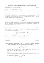
ones. In any case the parity of the cardinality of q −1 (0) and of q −1 (1) are the same,<br />
as illustrated in the following figure.<br />
t = 0 t = 1<br />
Figure 1.1: A one-dimensional cobordism<br />
Finally, an explicit computation shows that in the integrable situation the moduli<br />
space has exactly one element. Therefore q −1 (1) can not be empty either. An<br />
element of this moduli space provides the desired J-holomorphic approximation of<br />
ϕ. �<br />
1.5. Pseudo-analytic inequalities. In this section we lay the foundations for the<br />
study of critical points of pseudo-holomorphic maps. As this is a local question we<br />
take as domain the unit disk, ϕ : ∆ → (M,J). The main point of this study is that<br />
any singularity bears a certain kind of holomorphicity in itself, and the amount of<br />
holomorphicity indeed increases with the complexity of the singularity. The reason
SYMPLECTIC ISOTOPY 11<br />
for this to happen comes from the following series of results on differential inequalities<br />
for the ¯ ∂-operator. For simplicity of proof we formulate these only for functions with<br />
values in R rather than R n as needed and then comment on how to generalize to<br />
larger n.<br />
Lemma 1.9. Let f ∈ W 1,2 (∆) fulfill |∂¯zf| ≤ φ·|f| almost everywhere for φ ∈ L p (∆),<br />
p > 2. Then either f = 0 or there exist a uniquely determined integer µ and<br />
g ∈ W 1,p (∆), g(0) �= 0 with<br />
f(z) = z µ · g(z) almost everywhere.<br />
Proof. A standard elliptic bootstrapping argument shows f ∈ W 1,p (∆), see for example<br />
[IvSh1], Lemma 3.1.1,i. This step requires p > 2. Next comes a trick � attrib-<br />
�<br />
uted to Carleman to reduce to the holomorphic situation: By hypothesis � ∂¯zf<br />
�<br />
�<br />
� ≤ φ.<br />
We will recall in Proposition 2.1 below that ∂¯z : W 1,p (∆) → Lp (∆) is surjective.<br />
Hence there exists ψ ∈ W 1,p (∆) solving ∂¯zψ = ∂¯zf<br />
f . Then<br />
∂¯z(e −ψ f) = e −ψ (−∂¯zψ)f + e −ψ ∂¯zf = 0<br />
shows that e −ψ f is a holomorphic function (Carleman similarity principle). Now<br />
complex function theory tells us that e −ψ f = z µ ·h for h ∈ O(∆)∩W 1,p (∆), h(0) �= 0.<br />
Putting g = e ψ · h gives the required representation of f. �<br />
Remark 1.10. 1) As for an intrinsic interpretation of µ note that it is the intersection<br />
multiplicity of the graph of h with the graph of the zero function inside ∆×C at point<br />
(0,0). Multiplication by e ψ induces a homeomorphism of ∆ × C and transforms the<br />
graph of h into the graph of f. Hence µ is a topologically defined entity depending<br />
only on f.<br />
2) The Carleman trick replaces the use of a general removable singularities theorem<br />
for solutions of differential inequalities due to Harvey and Polking that was employed<br />
in [IvSh1], Lemma 3.1.1. Unlike the Carleman trick this method generalizes to maps<br />
f : ∆ → C n with n > 1. Another possibility that works also n > 1 is to use the<br />
Hartman-Wintner theorem on the polynomial behavior of solutions of certain partial<br />
differential equations in two variables, see e.g. [McSa3]. A third approach appeared<br />
in the printed version [IvSh2] of [IvSh1]; here the authors noticed that one can<br />
deduce a Carleman similarity principle also for maps f : ∆ → C n by viewing f as<br />
a holomorphic section of ∆ × C n , viewed as holomorphic vector bundle with nonstandard<br />
¯ ∂-operator. This is arguably the easiest method to deduce the result for<br />
all n. �<br />
A similar looking lemma of quite different flavor deduces holomorphicity up to<br />
some order from a polynomial estimate on |∂¯zf|. Again we took this from [IvSh1],<br />
but the proof given there makes unnecessary use of Lemma 1.9.<br />
Lemma 1.11. Let f ∈ L 2 (∆) fulfill |∂¯zf| ≤ φ · |z| ν almost everywhere for some<br />
φ ∈ L p (∆), p > 2 and ν ∈ N. Then either f = 0 or there exists P ∈ C[z], deg P ≤ ν<br />
and g ∈ W 1,p (∆), g(0) = 0 with<br />
f(z) = P(z) + z ν · g(z) almost everywhere.<br />
Proof. By induction over ν, the case ν = 0 being trivial. Assume the case ν − 1 is<br />
true. Elliptic regularity gives f ∈ W 1,p (∆). By the Sobolev embedding theorem f<br />
f
12 BERND SIEBERT <strong>AND</strong> GANG TIAN<br />
is Hölder continuous of exponent α = 1 − 2<br />
p ∈ (0,1). Hence f1 =<br />
� �<br />
� �<br />
|∂¯zf1| = � �<br />
� � ≤ φ · |z|ν−1 .<br />
∂¯zf<br />
z<br />
f − f(0)<br />
z<br />
is L 2 and<br />
Therefore induction applies to f1 and we see f1 = P1 +z ν−1 ·g with g of the required<br />
form. Plugging in the definition of f1 gives f = (f(0)+zP1)+z ν ·g, so P = f(0)+zP1<br />
is the correct definition of P.<br />
Remark 1.12. The lemma generalizes in a straightforward manner to maps f : ∆ →<br />
C n . In this situation the line C · P(0) has a geometric interpretation as complex<br />
tangent line of im(f) in f(0), which by definition is the limit of lines C·(f(z)−f(0)) ∈<br />
CP n−1 for z �= 0, z → 0. �<br />
Combining the two lemmas gives the following useful result, which again generalizes<br />
to maps f : ∆ → C n .<br />
Proposition 1.13. Let f ∈ L2 (∆) fulfill |∂¯zf| ≤ φ|z| ν |f| almost everywhere for<br />
φ ∈ Lp (∆), p > 2 and ν ∈ N. Then either f = 0 or there exist uniquely determined<br />
µ,ν ∈ N and P ∈ C[z], deg P ≤ ν, P(0) �= 0, g ∈ W 1,p (∆), g(0) = 0 with<br />
f(z) = z µ� P(z) + z ν · g(z) �<br />
almost everywhere.<br />
Proof. Lemma 1.9 gives f = z µ g. Now by hypothesis g also fulfills the stated<br />
estimate:<br />
�<br />
�<br />
|∂¯zg| = �<br />
∂¯zf<br />
� z µ<br />
� �<br />
� �<br />
�<br />
� ≤ φ|z|ν �<br />
f<br />
�z<br />
µ<br />
�<br />
�<br />
�<br />
� = φ|zν | · |g|.<br />
Thus replacing f by g reduces to the case f(0) �= 0 and µ = 0. The result then<br />
follows by Lemma 1.11 applied to f with φ replaced by φ · |f|. �<br />
2. Unobstructedness I: Smooth and nodal curves<br />
2.1. Preliminaries on the ¯ ∂-equation. The crucial tool to study the ¯ ∂-equation<br />
analytically is the inhomogeneous Cauchy integral formula. It says<br />
(2.1)<br />
∂∆<br />
f = Hf + T(∂¯zf)<br />
for all f ∈ C 1 (∆) with integral operators<br />
Hf(z) = 1<br />
�<br />
�<br />
f(w)<br />
1<br />
dw , Tg(z) =<br />
2πi w − z 2πi<br />
∆<br />
g(w)<br />
dw ∧ d ¯w .<br />
w − z<br />
(All functions in this section are C-valued.) The first operator H maps continuous<br />
functions defined on S 1 = ∂∆ to holomorphic functions on ∆. Continuity of Hf<br />
along the boundary is not generally true if f is just continuous. To understand this<br />
note that any f ∈ C 0 (S 1 ) can be written as a Fourier series �<br />
n∈Z anz n and then<br />
Hf = �<br />
n∈N anz n is the projection to the space of functions spanned by non-negative<br />
Fourier modes. This function need not be continuous.<br />
The integrand of the second integral operator T looks discontinuous, but in fact<br />
it is not as one sees in polar coordinates with center w = z. For differentiability<br />
properties one computes ∂¯zT = id from (2.1), while ∂zT = S with S the singular<br />
integral operator<br />
Sg(z) = 1<br />
2πi lim<br />
�<br />
g(w)<br />
dw ∧ d ¯w .<br />
ε→0 ∆\Bε(z) (w − z) 2
SYMPLECTIC ISOTOPY 13<br />
The Calderon-Zygmund theorem says that S is a continuous map from Lp (∆) to<br />
itself for 1 < p < ∞. Recall also that the Sobolev space W 1,p (∆) consists of Lp- functions with weak partial derivatives in Lp too. For p > 2 it holds 1 − 2<br />
p > 0,<br />
so the Sobolev embedding theorem implies that any f ∈ W 1,p (∆) has a continuous<br />
representative. Moreover, the map W 1,p (∆) → C0 (∆) thus defined is continuous.<br />
Thus (2.1) holds for f ∈ W 1,p (∆) for any p > 2. Summarizing the discussion, the<br />
Cauchy integral formula induces the following remarkable direct sum decomposition<br />
of W 1,p (∆).<br />
Proposition 2.1. Let 2 < p < ∞. Then (H, ¯ ∂) : W 1,p (∆) −→ � O(∆) ∩W 1,p (∆) � ×<br />
L p (∆) is an isomorphism. In particular, for any g ∈ L p (∆) there exists f ∈ W 1,p (∆)<br />
with ∂¯zf = g.<br />
Thus any f ∈ W 1,p (∆) can be written in the form h+T(∂¯zf) with h holomorphic<br />
in ∆ and continuously extending to ∆ and T(∂¯zf)|∂∆ gathering all negative Fourier<br />
coefficients of f| ∆ .<br />
2.2. The normal ¯ ∂-operator. We have already described pseudo-holomorphic<br />
maps by a non-linear PDE. One trivial variation of a pseudo-holomorphic map is<br />
by reparametrization. It is sometimes useful to get rid of this part, especially if one<br />
is interested in pseudo-holomorphic curves rather than pseudo-holomorphic maps.<br />
This is achieved by the normal ¯ ∂-operator that we now introduce.<br />
Recall that for a pseudo-holomorphic map ϕ : Σ → M the operator ¯ ∂ϕ,J from<br />
(1.1) in §1.3 defines a natural holomorphic structure on ϕ ∗ TM compatible with the<br />
holomorphic structure on TΣ. In fact, a straightforward computation shows<br />
Dϕ ◦ ¯ ∂TΣ = ¯ ∂ϕ,J ◦ Dϕ.<br />
If ϕ is an immersion we thus obtain a short exact sequence of holomorphic vector<br />
bundles over Σ<br />
0 −→ TΣ −→ ϕ ∗ (TM) −→ N −→ 0.<br />
This sequence defines the normal bundle N along ϕ. If ϕ has critical points it is<br />
still possible to define a normal bundle as follows. For a complex vector bundle V<br />
denote by O(V ) the sheaf of holomorphic sections of V . While at critical points<br />
Dϕ : TΣ → ϕ ∗ TM is not injective the map of sheaves O(TΣ) → O(ϕ ∗ TM) still is.<br />
As an example consider ϕ(t) = (t 2 ,t 3 ) as map from ∆ to C 2 with standard complex<br />
structure. Then<br />
(2.2)<br />
Dϕ(∂t) = 2t ∂z + 3t 2 ∂w,<br />
and as germ of holomorphic function the right-side is non-zero. Thus in any case we<br />
obtain a short exact sequence of sheaves of OΣ-modules<br />
(2.3)<br />
0 −→ O(TΣ) Dϕ<br />
−→ O(ϕ ∗ TM) −→ N −→ 0.<br />
From the definition, N is just some coherent sheaf on Σ. But on a Riemann surface<br />
any coherent sheaf splits uniquely into a skyscraper sheaf (discrete support) and the<br />
sheaf of sections of a holomorphic vector bundle. Thus we may write<br />
N = N tor ⊕ O(N)<br />
for some holomorphic vector bundle N. We call N the normal sheaf along ϕ and<br />
N the normal bundle. The skyscraper sheaf N tor is the subsheaf of N generated<br />
by sections that are annihilated by multiplication by some non-zero holomorphic
14 BERND SIEBERT <strong>AND</strong> GANG TIAN<br />
function (“torsion sections”). In our example ϕ(t) = (t 2 ,t 3 ) the section v = 2∂z +<br />
3t ∂w of ϕ ∗ TM is contained in the image of O(TΣ) for t �= 0, but not at t = 0,<br />
while tv = Dϕ(∂t). In fact, N tor is isomorphic to a copy of C over t = 0 generated<br />
by the germ of v at 0. Then N is the holomorphic line bundle generated by any<br />
a(t)∂z + b(t)∂w with b(0) �= 0.<br />
As a simple but very powerful application of the normal sequence (2.3) we record<br />
the genus formula for pseudo-holomorphic curves in dimension four.<br />
Proposition 2.2. Let (M,J) be an almost complex 4-manifold and C ⊂ M an<br />
irreducible pseudo-holomorphic curve. Then<br />
with equality if and only if C is smooth.<br />
2g(C) − 2 ≤ c1(M) · C + C · C,<br />
Proof. Let ϕ : Σ → M be the pseudo-holomorphic map with image C. Since<br />
deg TΣ = 2g(C) − 2 the normal sequence (2.3) shows<br />
2g(C) − 2 = deg ϕ ∗ TM + deg N + lg N tor = c1(M) · C + deg N + lg N tor .<br />
Here lg N tor is the sum of the C-vector space dimensions of the stalks of N. This<br />
term vanishes iff N = 0, that is, iff ϕ is an immersion. The degree of N equals C ·C<br />
if C is smooth and drops by the self-intersection number of ϕ in the immersed case.<br />
By the PDE description of the space of pseudo-holomorphic maps from a unit disk<br />
to M, it is not hard to show that locally in Σ any pseudo-holomorphic map Σ → M<br />
can be perturbed to a pseudo-holomorphic immersion. At the expense of changing<br />
J away from the singularities of C slightly this statement globalizes. This process<br />
does not change any of g(C), c1(M) · C and C · C. Hence the result for general C<br />
follows from the immersed case. �<br />
To get rid of N tor it is convenient to go over to meromorphic sections of TΣ with<br />
poles of order at most ordP Dϕ in a critical point P of Dϕ. In fact, the sheaf<br />
of such meromorphic sections is the sheaf of holomorphic sections of a line bundle<br />
that we conveniently denote TΣ[A], where A is the divisor �<br />
P ∈crit(ϕ) (ordP Dϕ) · P.<br />
Then TΣ[A] = kern(ϕ ∗ TM → N) and hence we obtain the short exact sequence of<br />
holomorphic vector bundles<br />
0 −→ TΣ[A] Dϕ<br />
−→ ϕ ∗ TM −→ N −→ 0.<br />
Thus by (2.2) together with R◦Dϕ = 0 the operator Dϕ,J = ¯ ∂ϕ,J+R : W 1,p (ϕ ∗ TM) →<br />
L p (ϕ ∗ TM ⊗ Λ 0,1 ) fits into the following commutative diagram with exact rows.<br />
0 −−−−→ W 1,p (TΣ[A]) −−−−→ W 1,p (ϕ∗TM) −−−−→ W 1,p (N) −−−→ 0<br />
⏐<br />
⏐<br />
⏐<br />
⏐<br />
⏐<br />
⏐<br />
¯∂TΣ �<br />
�Dϕ,J<br />
�DN ϕ,J<br />
0 −−−−→ L p (TΣ[A] ⊗ Λ 0,1 ) −−−−→ L p (ϕ ∗ TM ⊗ Λ 0,1 ) −−−−→ L p (N ⊗ Λ 0,1 ) −−−→ 0<br />
This defines the normal ¯ ∂J-operator D N ϕ,J . As with Dϕ,J we have the decomposition<br />
D N ϕ,J = ¯ ∂N + RN into complex linear and a zero order complex anti-linear part. By<br />
the snake lemma the diagram readily induces the long exact sequence<br />
0 −−−−→ H 0 (TΣ[A]) −−−−→ kern Dϕ,J −−−−→ kern D N ϕ,J<br />
−−−−→ H 1 (TΣ[A]) −−−−→ coker Dϕ,J −−−−→ coker D N ϕ,J<br />
−−−→ 0
SYMPLECTIC ISOTOPY 15<br />
The cohomology groups on the left are Dolbeault cohomology groups for the holomorphic<br />
vector bundle TΣ[A] or sheaf cohomology groups of the corresponding coherent<br />
sheaves. Forgetting the twist by A then gives the following exact sequence.<br />
(2.4)<br />
0 −−−→ H 0 (TΣ) −−−−→ kern Dϕ,J −−−−→ kern D N ϕ,J ⊕ H0 (N tor )<br />
−−−→ H 1 (TΣ) −−−−→ coker Dϕ,J −−−−→ coker D N ϕ,J −−−→ 0<br />
The terms in this sequence have a geometric interpretation. Each column is associated<br />
to a deformation problem. The left-most column deals with deformations of<br />
Riemann surfaces: H0 (TΣ) is the space of holomorphic vector fields on Σ. It is trivial<br />
except in genera 0 and 1, where it gives infinitesimal holomorphic reparametrizations<br />
of ϕ. As already mentioned in §1.3, the space H1 (TΣ) is isomorphic to the<br />
space of holomorphic quadratic differentials via Serre-duality and hence describes<br />
the tangent space to the Riemann or Teichmüller space of complex structures on Σ.<br />
Every element of this space is the tangent vector of an actual one-parameter family<br />
of complex structures on Σ — this deformation problem is unobstructed.<br />
The middle column covers the deformation problem of ϕ as pseudo-holomorphic<br />
curve with almost complex structures both on M and on Σ fixed. In fact, Dϕ,J is the<br />
linearization of the Fredholm map describing the space of pseudo-holomorphic maps<br />
(Σ,j) → (M,J) with fixed almost complex structures (see proof of Proposition 1.3).<br />
If coker Dϕ,J �= 0 this moduli space might not be smooth of the expected dimension<br />
ind(Dϕ,J), and this is then an obstructed deformation problem.<br />
The maps from the left column to the middle column also have an interesting<br />
meaning. On the upper part, H0 (TΣ) → kern Dϕ,J describes infinitesimal holomorphic<br />
reparametrizations as infinitesimal deformations of ϕ. On the lower part, the<br />
image of H1 (TΣ) in coker Dϕ,J exhibits those obstructions of the deformation problem<br />
of ϕ with fixed almost complex structures that can be killed by variations of the<br />
complex structure of Σ.<br />
The right column is maybe the most interesting. First, there are no obstructions<br />
to the deformations of ϕ as J-holomorphic map iff coker DN ϕ,J = 0, provided we allow<br />
variations of the complex structure of Σ. Thus when it comes to the smoothness<br />
of the moduli space relative J then coker D N ϕ,J<br />
is much more relevant than the<br />
more traditional coker Dϕ,J. Finally, the term on the upper right corner consists<br />
of two terms, with H0 (N tor ) reflecting deformations of the singularities. In fact,<br />
infinitesimal deformations with vanishing component on this part can be realized<br />
by sections of ϕ∗TM with zeros of the same orders as those of Dϕ. This follows<br />
directly from the definition of N tor . Such deformations are exactly those keeping<br />
the number of critical points of ϕ. Note that while N tor does not explicitly show up in<br />
the obstruction space coker DN ϕ,J , it does influence this space by lowering the degree<br />
of N. The exact sequence also gives the (non-canonical) direct sum decomposition<br />
kern D N ϕ,J ⊕ H0 (N tor ) = � kern Dϕ,J/H 0 (TΣ) � ⊕ kern � H 1 �<br />
(TΣ) → coker Dϕ,J .<br />
The decomposition on the right-hand side mixes local and global contributions. The<br />
previous discussion gives the following interpretation: kern Dϕ,J/H 0 (TΣ) is the space<br />
of infinitesimal deformations of ϕ as J-holomorphic map modulo biholomorphisms;<br />
kern � H1 �<br />
(TΣ) → coker Dϕ,J is the tangent space to the space of complex structures<br />
on Σ that can be realized by variations of ϕ as J-holomorphic map.<br />
Summarizing this discussion, it is the right column that describes the moduli<br />
space of pseudo-holomorphic maps for fixed J. In particular, if coker DN ϕ,J = 0 then
16 BERND SIEBERT <strong>AND</strong> GANG TIAN<br />
the moduli space MJ ⊂ M of J-holomorphic maps Σ → M for arbitrary complex<br />
structures on Σ is smooth at (ϕ,J,j) with tangent space<br />
T MJ,(ϕ,J,j) = kern D N ϕ,J ⊕ H 0 (N tor ).<br />
2.3. Immersed curves. If dim M = 4 and ϕ : Σ → M is an immersion then N is<br />
a holomorphic line bundle and<br />
N ⊗ TΣ ≃ ϕ ∗ (det TM).<br />
Here TM is taken as complex vector bundle. From this we are going to deduce a<br />
cohomological criterion for surjectivity of<br />
By elliptic theory the cokernel of D N ϕ,J<br />
operator<br />
D N ϕ,J = ¯ ∂ + R : W 1,p (N) −→ L p (N ⊗ Λ 0,1 ).<br />
is dual to the kernel of its formal adjoint<br />
(D N ϕ,J )∗ : W 1,p (N ∗ ⊗ Λ 1,0 ) −→ L p (N ∗ ⊗ Λ 1,1 ).<br />
Note that (D N ϕ,J )∗ = ¯ ∂ −R ∗ is also of Cauchy-Riemann type. Now in dimension 4 the<br />
bundle N is a holomorphic line bundle over Σ. In a local holomorphic trivialization<br />
(D N ϕ,J )∗ therefore takes the form f ↦→ ¯ ∂f +αf +β ¯ f for some functions α,β. Solutions<br />
of such equations are called pseudo-analytic. While related this notion predates<br />
pseudo-holomorphicity and should not be mixed up with it.<br />
Lemma 2.3. Let α,β ∈ L p (∆) and let f ∈ W 1,p (∆) \ {0} fulfill<br />
∂¯zf + αf + β ¯ f = 0.<br />
Then all zeros of f are isolated and positive.<br />
Proof. This is another application of the Carleman trick, cf. proof of Lemma 1.9.<br />
Replacing α by α + β · ¯ f/f reduces to the case β = 0. Note that ¯ f/f is bounded, so<br />
β · ¯ f/f stays in L p . By Proposition 2.1 there exists g ∈ W 1,p (∆) solving ∂¯zg = α.<br />
Then<br />
∂¯z(e g f) = e g (∂¯zg · f + ∂¯zf) = e g (αf + ∂¯zf) = 0.<br />
Thus the diffeomorphism Ψ : (z,w) ↦→ (z,e g(z) w) transforms the graph of f into the<br />
graph of a holomorphic function. �<br />
Here is the cohomological unobstructedness theorem for immersed curves.<br />
Proposition 2.4. Let (M,J) be a 4-dimensional almost complex manifold,and ϕ :<br />
Σ → M an immersed J-holomorphic curve with c1(M) · [C] > 0. Then the moduli<br />
space MJ of J-holomorphic maps to M is smooth at (j,ϕ,J).<br />
Proof. By the previous discussion the result follows once we show the vanishing of<br />
kern(D N ϕ,J )∗ . An element of this space is a section of the holomorphic line bundle<br />
N ∗ ⊗ Λ 1,0 over Σ of degree<br />
deg(N ∗ ⊗ Λ 1,0 ) = deg(det T ∗ M |C) = −c1(M) · [C] < 0.<br />
In a local holomorphic trivialization it is represented by a pseudo-analytic function.<br />
Thus by Lemma 2.3 and the degree computation it has to be identically zero. �
SYMPLECTIC ISOTOPY 17<br />
2.4. Smoothings of nodal curves. A pseudo-holomorphic curve C ⊂ M is a<br />
nodal curve if all singularities of C are transversal unions of two smooth branches.<br />
It is natural to consider a nodal curve as the image of an injective map from a<br />
nodal Riemann surface. A nodal Riemann surface is a union of Riemann surfaces<br />
Σi with finitely many disjoint pairs of points identified. The identification map<br />
ˆΣ := �<br />
i Σi → Σ from the disjoint union is called normalization. (This notion<br />
has a more precise meaning in complex analysis.) A map ϕ : Σ → M is pseudoholomorphic<br />
if it is continuous and if the composition ˆϕ : ˆ Σ → Σ → M is pseudoholomorphic.<br />
Analogously one defines W 1,p-spaces for p > 2.<br />
For a nodal curve C it is possible to extend the above discussion to include<br />
topology change by smoothing the nodes, as in zw = t for (z,w) ∈ ∆ × ∆ and t<br />
the deformation parameter. This follows from the by now well-understood gluing<br />
construction for pseudo-holomorphic maps. There are various ways to achieve this,<br />
see for example [LiTi], [Si]. They share a formulation by a family of non-linear<br />
Fredholm operators<br />
�<br />
i<br />
H 1 (TΣi ) × W 1,p (ϕ ∗ TM) −→ L p (ϕ ∗ TM ⊗ Λ 0,1 ),<br />
parametrized by l = ♯nodes gluing parameters (t1,...,tl) ∈ C l of sufficiently small<br />
norm. (The definitions of W 1,p and L p near the nodes vary from approach to approach.)<br />
Thus fixed (t1,...,tl) gives the deformation problem with given topological<br />
type as discussed above, and putting ti = 0 means keeping the i-th node. The<br />
linearization D ′ ϕ,J of this operator for (t1,...,tl) = 0 and fixed almost complex<br />
structures fits into a diagram very similar to the one above:<br />
0 −−−−→ W 1,p (TΣ[A]) −−−−→ W 1,p (ϕ ∗ TM) −−−−→ W 1,p (N ′ ) −−−−→ 0<br />
⏐ ¯∂TΣ �<br />
⏐<br />
�D ′ ϕ,J<br />
⏐<br />
�D<br />
0 −−−−→ L p (TΣ[A] ⊗ Λ 0,1 ) −−−−→ L p (ϕ ∗ TM ⊗ Λ 0,1 ) −−−−→ L p (N ′ ⊗ Λ 0,1 ) −−−−→ 0.<br />
In the right column N ′ denotes the image of N under the normalization map:<br />
N ′ := �<br />
i<br />
ϕ ∗ i TM/Dϕi(TΣi ).<br />
Thus N ′ is a holomorphic line bundle on Σ only away from the nodes, while near<br />
a node it is a direct sum of line bundles on each of the two branches. Note that<br />
surjectivity of W 1,p (Σ,ϕ ∗ TM) → W 1,p (Σ,N ′ ) is special to the nodal case in dimension<br />
4 since it requires the tangent spaces of the branches at a node P ∈ ϕ(C) to<br />
generate TM,P. A crucial observation then is that the obstructions to this extended<br />
deformation problem can be computed on the normalization:<br />
N ′<br />
coker Dϕ,J = coker DNˆϕ,J .<br />
This follows by chasing the diagrams. Geometrically the identity can be understood<br />
by saying that it is the same to deform ϕ as pseudo-holomorphic map or to deform<br />
each of the maps Σi → M separately. In fact, the position of the identification points<br />
of the Σi are uniquely determined by the maps to M. In view of the cohomological<br />
unobstructedness theorem and the implicit function theorem relative J × C l we<br />
obtain the following strengthening of Proposition 2.4.<br />
N ′<br />
ϕ,J
18 BERND SIEBERT <strong>AND</strong> GANG TIAN<br />
Proposition 2.5. [Sk] Let C ⊂ M be a nodal J-holomorphic curve on an almost<br />
complex 4-manifold (M,J), C = � Ci. Assume that c1(M)·Ci > 0 for every i. Then<br />
the moduli space of J-holomorphic curves homologous to C is a smooth manifold of<br />
real dimension c1(M) · C + C · C. The subset parametrizing nodal curves is locally a<br />
transversal union of submanifolds of real codimension 2. In particular, there exists<br />
a sequence of smooth J-holomorphic curves Cn ⊂ M with Cn → C in the Hausdorff<br />
sense (C can be smoothed), and such smoothings are unique up to isotopy through<br />
smooth J-holomorphic curves. �<br />
3. The theorem of Micallef and White<br />
3.1. Statement of theorem. In this section we discuss the theorem of Micallef<br />
and White on the holomorphicity of germs of pseudo-holomorphic curves up to C 1 -<br />
diffeomorphism. The precise statement is the following.<br />
Theorem 3.1. (Micallef and White [MiWh], Theorem 6.2.) Let J be an almost<br />
complex structure on a neighborhood of the origin in R 2n with J |0 = I, the standard<br />
complex structure on C n = R 2n . Let C ⊂ R 2n be a J-holomorphic curve with 0 ∈ C.<br />
Then there exists a neighborhood U of 0 ∈ R 2n and a C 1 -diffeomorphism Φ : U →<br />
V ⊂ C n , Φ(0) = 0, DΦ |0 = id, such that Φ(C) ⊂ V is defined by complex polynomial<br />
equations. In particular, Φ(C) is a holomorphic curve.<br />
The proof in loc. cit. might seem a bit computational on first reading, but the<br />
basic idea is in fact quite elegant and simple. As it is one substantial ingredient in<br />
our proof of the isotopy theorem, we include a discussion here. For simplicity we<br />
restrict to the two-dimensional, pseudo-holomorphically fibered situation, just as in<br />
§1.4.1. In other words, there are complex coordinates z,w with (z,w) ↦→ z pseudoholomorphic.<br />
Then w can be chosen in such a way that T 1,0<br />
M = C ·(∂¯z +b∂w)+C·∂ ¯w<br />
for a C-valued function b with b(0,0) = 0. This will be enough for our application<br />
and it still captures the essentials of the fully general proof.<br />
3.2. The case of tacnodes. Traditionally a tacnode is a higher order contact point<br />
of a union of smooth holomorphic curves, its branches. The same definition makes<br />
sense pseudo-holomorphically. We assume this tangent to be w = 0. Then the i-th<br />
branch of our pseudo-holomorphic tacnode is the image of<br />
∆ −→ C 2 , t ↦−→ (t,fi(t)),<br />
with fi(0) = 0, Dfi|0 = 0. The pseudo-holomorphicity equation takes the form<br />
∂¯tfi = b(t,fi(t)). For i �= j this gives the equation<br />
0 = � ∂¯tfj − b(t,fj) � − � ∂¯tfi − b(t,fi) �<br />
= ∂¯t(fj − fi) − b(t,fj) − b(t,fi)<br />
· (fj − fi).<br />
fj − fi<br />
Now � b(t,fj) − b(t,fi) � /(fj − fi) is bounded, and hence fj − fi is another instance<br />
of a pseudo-analytic function. The Carleman trick in Lemma 2.3 now implies that<br />
fi and fj osculate only to finite order. (This also follows from Aronszajn’s unique<br />
continuation theorem [Ar].)<br />
On the other hand, if fj −fi = O(|t| n ) then |∂¯t(fj −fi)| = � � b(t,fi(t))−b(t,fj(t)) � � =<br />
O(|t| n ) by pseudo-holomorphicity and hence, by Lemma 1.11<br />
(3.1)<br />
fj(t) − fi(t) = at n + o(|t| n ).
SYMPLECTIC ISOTOPY 19<br />
The polynomial leading term provides the handle to holomorphicity. The diffeomorphism<br />
Φ will be of the form<br />
Φ(z,w) = (z,w − E(z,w)).<br />
To construct E(z,w) consider the approximations<br />
fi,n = M.V. � �<br />
fj<br />
�fj − fi = o(|t| n ) �<br />
to fi, for every i and n ≥ 1. M.V. stands for the arithmetic mean. Because we<br />
are dealing with a tacnode, fi,1 = fj,1 for every i,j, and by finiteness of osculation<br />
orders, there exists N with fi,n = fi for every n ≥ N. Now (3.1) gives ai,n ∈ C and<br />
functions Ei,n with<br />
Summing from n = 1 to N shows<br />
(3.2)<br />
fi,n − fi,n−1 = ai,nt n + Ei,n(t), Ei,n(t) = o(|t| n ).<br />
fi =<br />
N�<br />
ai,nt n + fi,1(t) +<br />
n=2<br />
N�<br />
Ei,n(t).<br />
The rest is a matter of merging the various Ei,n into E(z,w) to achieve Φ(t,fi(t)) =<br />
(t, �N n=2 ai,ntn ). We are going to set E = �N i=1 Ei with Ei(z,w) = Ei,n(z) in a strip<br />
osculating to order n to the graph of fi,n. More precisely, choose a smooth cut-off<br />
function ρ : R≥0 → [0,1] with ρ(s) = 1 for s ∈ [0,1/2] and ρ(s) = 0 for s ≥ 1. Then<br />
for n = 1 define<br />
�<br />
|w|<br />
E1(z,w) = ρ<br />
|z| 3/2<br />
�<br />
· fi,1(z).<br />
The exponent 3/2 may be replaced by any number in (1,2). For n ≥ 2 take<br />
⎧ �<br />
⎨ |w − fi,n(z)|<br />
ρ<br />
En(z,w) = ε|z|<br />
⎩<br />
n<br />
�<br />
· Ei,n(z), |w − fi,n(z)| ≤ ε|z| n<br />
0, otherwise.<br />
To see that this is well-defined for ε and |z| sufficiently small note that by construction<br />
fi,n and fj,n osculate polynomially to dominant order. If this order is larger<br />
than n then fi,n = fj,n. Otherwise |fj,n(z) − fi,n(z)| > ε|z| n for ε and |z| sufficiently<br />
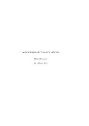
small. See Figure 3.1 for illustration.<br />
supp E4<br />
supp E1<br />
Figure 3.1: The supports of En. Figure 3.2: Different tangent lines.<br />
n=2
20 BERND SIEBERT <strong>AND</strong> GANG TIAN<br />
The distinction between the cases n = 1 and n > 1 at this stage could be avoided by<br />
formally setting Ei,1 = fi,1. However, to also treat branches with different tangents<br />
later on, we want Φ to be the identity outside a region of the form |z| ≤ |w| a with<br />
a > 1.<br />
Finally note that by construction En(t,fi(t)) = Ei,n(t), and hence<br />
Φ(t,fi(t)) = � t,fi(t) − �<br />
En(t,fi(t)) �<br />
= � t,fi(t) −<br />
n<br />
N�<br />
n=2<br />
Ei,n(t) − fi,1(t) � (3.2)<br />
= (t,<br />
N�<br />
n=1<br />
ai,nt n ).<br />
This finishes the proof of Theorem 3.1 for the case of tacnodes under the made<br />
simplifying assumptions.<br />
As for differentiability it is clear that Φ is smooth away from (0,0). But ∂wEn<br />
involves the term<br />
���� �<br />
|w − fi,n|<br />
∂ ¯wρ<br />
ε · |z| n<br />
�� �<br />
�� = 1<br />
|z| n · o(|z|n ) = o(1).<br />
Thus ϕ may only be C 1 .<br />
3.3. The general case. In the general case the branches of C are images of pseudoholomorphic<br />
maps<br />
∆ −→ C 2 , t ↦−→ (t Qi ,fi(t)),<br />
for some Qi ∈ N. Note our simplifying assumption that the projection onto the first<br />
coordinate be pseudo-holomorphic. By composing with branched covers t ↦→ tmi we may assume Qi = Q for all i. The pseudo-holomorphicity equation then reads<br />
∂¯tfi = Q¯t Qb(t,fi(t)). The proof now proceeds as before but we deal with multivalued<br />
functions Ei,n of z. A simple way to implement this is by enlarging the set<br />
of functions fi by including compositions with t ↦→ ζt for all Q-th roots of unity ζ.<br />
The definition of En(z,w) then reads<br />
⎧ �<br />
⎨ |w − fi,n(t)|<br />
ρ<br />
En(z,w) = ε|t|<br />
⎩<br />
n<br />
�<br />
· Ei,n(t), |w − fi,n(t)| ≤ ε|z| n<br />
0, otherwise,<br />
for any t with t Q = z. This is well-defined as before since the set of functions fi is<br />
invariant under composition with t ↦→ ζt whenever ζ Q = 1.<br />
Finally, if C has branches with different tangent lines do the construction for the<br />
union of branches with given tangent line separately. The diffeomorphisms obtained<br />
in this way are the identity outside of trumpet-like sets osculating to the tangent<br />
lines as in Figure 3.2. Hence their composition maps each branch to an algebraic<br />
curve as claimed in the theorem.<br />
4. Unobstructedness II: The integrable case<br />
4.1. Motivation. We saw in Section 2 that if c1(M) evaluates strictly positively<br />
on a smooth pseudo-holomorphic curve in a four-manifold then this curve has unobstructed<br />
deformations. The only known generalizations to singular curves rely on<br />
parametrized deformations. These deformations preserve the geometric genus and,<br />
by the genus formula, lead at best to a nodal curve. Unobstructedness in this restricted<br />
class of deformations is a stronger statement, which thus requires stronger
SYMPLECTIC ISOTOPY 21<br />
assumptions. In particular, the types of the singular points enter as a condition, and<br />
this limits heavily the usefulness of such results for the isotopy problem. Note these<br />
problems do already arise in the integrable situation. For example, not every curve<br />
on a complex surface can be deformed into a curve of the same geometric genus with<br />
only nodes as singularities. This is a fact of life and can not be circumvented by<br />
clever arguments.<br />
Thus we need to allow an increase of geometric genus. There are two points of<br />
views for this. The first one looks at a singular pseudo-holomorphic curve as the<br />
image of a pseudo-holomorphic map from a nodal Riemann surface, as obtained<br />
by the Compactness Theorem (Section 6). While this is a good point of view for<br />
many general problems such as defining Gromov-Witten invariants, we are now<br />
dealing with maps from a reducible domain to a complex two-dimensional space.<br />
This has the effect that (total) degree arguments alone as in Section 2 do not give<br />
good unobstructedness results. For example, unobstructedness fails whenever the<br />
limit stable map contracts components of higher genus. Moreover, it is not hard to<br />
show that not all stable maps allowed by topology can arise. There are subtle and<br />
largely ununderstood analytical obstructions preventing this. Again both problems<br />
are inherited from the integrable situation. A characterization of holomorphic or<br />
algebraic stable maps that can arise as limit is an unsolved problem in algebraic<br />
geometry. There is some elementary discussion on this in the context of stable<br />
reduction in [HaMo]. If a good theory of unobstructedness in the integrable case<br />
from the point of view of stable maps was possible it would likely generalize to the<br />
pseudo-holomorphic setting. Unfortunately, such theory is not in sight.<br />
The second point of view considers deformations of the limit as a cycle. The<br />
purpose of this section is to prove unobstructedness in the integrable situation under<br />
the mere assumption that every component evaluates strictly positively on c1(M).<br />
This is the direct analogue of Proposition 2.4. Integrability is essential here as<br />
the analytic description of deformations of pseudo-holomorphic cycles becomes very<br />
singular under the presence of multiple components, see [SiTi2].<br />
4.2. Special covers. We now begin with the proper content of this section. Let<br />
X be a complex surface, not necessarily compact but without boundary. In our<br />
application X will be a tubular neighborhood of a limit pseudo-holomorphic cycle<br />
in a rational ruled almost complex four-manifold M, endowed with a different, integrable<br />
almost complex structure. Let C = �<br />
i miCi be a compact holomorphic cycle<br />
of complex dimension one. We assume C to be effective, that is mi > 0 for all i.<br />
There is a general theory on the existence of moduli spaces of compact holomorphic<br />
cycles of any dimension, due to Barlet [Bl]. For the case at hand it can be greatly<br />
simplified and this is what we will do in this section.<br />
The approach presented here differs from [SiTi3], §4 in being strictly local around<br />
C. This has the advantage to link the linearization of the modeling PDE to cohomology<br />
on the curve very directly. However, such a treatment is not possible if C<br />
contains fibers of our ruled surface M → S2 , and then the more global point of view<br />
of [SiTi3] becomes necessary.<br />
The essential simplification is the existence of special covers of a neighborhood of<br />
|C| = �<br />
i Ci.<br />
Hypothesis 4.1. There exists an open cover U = {Uµ} of a neighborhood of C in<br />
M with the following properties:
22 BERND SIEBERT <strong>AND</strong> GANG TIAN<br />
(1) cl(Uµ) ≃ Aµ × ¯ ∆, where Aµ is a compact, connected Riemann surface with<br />
non-empty boundary and ¯ ∆ ⊂ C is the closed unit disk.<br />
(2) (Aµ × ∂∆) ∩ |C| = ∅.<br />
(3) Uκ ∩Uµ ∩Uν = ∅ for any pairwise different κ,µ,ν. The fiber structures given<br />
by projection to Aµ are compatible on overlaps. �<br />
The symbol “≃” denotes biholomorphism. The point of these covers is that on Uµ<br />
there is a holomorphic projection Uµ → inn(Aµ) with restriction to |C| proper and<br />
with finite fibers, hence a branched covering. Such cycles in Aµ × C of degree b over<br />
Aµ have a description by b holomorphic functions via Weierstraß polynomials, see<br />
below. Locally this indeed works in any dimension. But it is generally impossible<br />
to make the projections match on overlaps as required by (3), not even locally and<br />
for smooth C. The reason is that the analytic germ of M along C need not be<br />
isomorphic to the germ of the holomorphic normal bundle along the zero section.<br />
This almost always fails in the positive (“ample”) case that we are interested in, see<br />
[La]. For our application to cycles in ruled surfaces, however, we can use the bundle<br />
projection, provided C does not contain fiber components. Without this assumption<br />
the arguments below still work but require a more difficult discussion of change of<br />
projections, as in [Bl]. As the emphasis of these lectures is on explaining why things<br />
are true rather than generality we choose to impose this simplifying assumption.<br />
Another, more severe, simplification special to one-dimensional C is that we do<br />
not allow triple intersections. This implies that Aµ can not be contractible for all µ<br />
unless all components of C are rational, and hence our charts have a certain global<br />
flavor. Under the presence of triple intersections it seems impossible to get our direct<br />
connection of the modeling of the moduli space with cohomological data on C.<br />
Lemma 4.2. Assume there exists a map p : M → S with dim S = 1 such that p is<br />
a holomorphic submersion near |C| and no component of |C| contains a connected<br />
component of a fiber of p. Then Hypothesis 4.1 is fulfilled.<br />
Proof. Denote by Z ⊂ M the finite set of singular points of |C| and of critical points<br />
of the projection |C| → S. Add finitely many points to Z to make sure that Z<br />
intersects each irreducible component of |C|. For P ∈ |C| let F = p −1 (p(P)) be the<br />
fiber through P. Then F ∩ |C| is an analytic subset of F that by hypothesis does<br />
not contain a connected component of F. Since F is complex one-dimensional P is<br />
an isolated point of F ∩ C. Because p is a submersion there exists a holomorphic<br />
chart (z,w) : U(P) → C 2 in a neighborhood of P in M with (z,w)(P) = 0 and<br />
z = const describing the fibers of p. We may assume U(P) to be so small that |C|<br />
is the zero locus of a holomorphic function h defined on all of U(P). Let ε > 0<br />
be such that F ∩ w −1 (Bε(0)) = {P }. Then min � |f(0,w)| � � |w| = ε � > 0. Hence<br />
for δ > 0 sufficiently small min{|f(z,w)| | |w| = ε, |z| ≤ δ} remains nonzero. This<br />
shows |C| ∩ (z,w) −1 (Bδ(0) × ∂Bε(0)) = ∅. This verifies Hypothesis 4.1,1 and 2 for<br />
U(P), while the compatibility of fiber structures in 4.1,3 holds by construction. This<br />
defines elements U1,... ,U♯Z of the open cover U intersecting Z.<br />
To finish the construction we define one more open set U0 as follows. This construction<br />
relies on Stein theory, see e.g. [GrRe] or [KpKp] for the basics. (With<br />
some effort this can be replaced by more elementary arguments, but it does not<br />
seem worthwhile doing here for a technical result like this.) Choose a Riemannian<br />
metric on M. Let δ be so small that B2δ(Z) ⊂ �<br />
ν≥1 Uν. Since we have chosen Z to<br />
intersect each irreducible component of |C|, the complement |C|\cl Bδ(Z) is a union
SYMPLECTIC ISOTOPY 23<br />
of open Riemann surfaces. Thus |C|\cl Bδ(Z) is a Stein submanifold of M \cl Bδ(Z),<br />
hence has a Stein neighborhood W ⊂ M \ cl Bδ(Z). Now every hypersurface in a<br />
Stein manifold is defined by one global holomorphic function, say f in our case. So<br />
f is a global version of the fiber coordinate w before. Then for δ sufficiently small<br />
the projection<br />
U0 := � P ∈ W \ cl B 3δ/2(Z) � � |f(P)| < δ � p<br />
−→ S<br />
factors holomorphically through π : U0 → |C| \ cl B3δ/2(Z). This is an instance<br />
of so-called Stein factorization, which contracts the connected components of the<br />
fibers of a holomorphic map. Choosing δ even smaller this factorization gives a<br />
biholomorphism<br />
(π,f)<br />
U0 −→ |C| \ cl Bδ(Z) × ∆<br />
extending to cl(U0). Hence U0,U1,... ,U♯Z provides the desired open cover U . �<br />
4.3. Description of deformation space. Having a cover fulfilling Hypothesis 4.1<br />
it is easy to describe the moduli space of small deformations of C as the fiber of<br />
a holomorphic, non-linear Fredholm map. We use Čech notation Uµν = Uµ ∩ Uν,<br />
Uκµν = Uκ ∩ Uµ ∩ Uν. Write Vµ = inn(Aµ). Fix p > 2 and denote by O p (Vµ)<br />
the space of holomorphic functions on inn(Vµ) of class L p . This is a Banach space<br />
with the L p -norm defined by a Riemannian metric on Aµ, chosen once and for all.<br />
Similarly define O p (Vµν) and O p (Vκµν).<br />
To describe deformations of C let us first consider the local situation on Vµ ×∆ ⊂<br />
M. For this discussion we drop the index µ. Denote by w the coordinate on the unit<br />
disk. For any holomorphic cycle C ′ on V ×∆ with |C ′ |∩(V ×∂∆) = ∅ the Weierstraß<br />
preparation theorem gives bounded holomorphic functions a1,... ,ab ∈ O p (V ) with<br />
w b +a1w b−1 +...+ab = 0 describing C ′ , see e.g. [GrHa]. Here b is the relative degree<br />
of C ′ over V , and everything takes multiplicities into account. The tuple (a1,...,ab)<br />
should be thought of as a holomorphic map from V to the b-fold symmetric product<br />
Sym b C of C with itself.<br />
Digression on Sym b C. By definition Sym b C is the quotient of C × ... × C by the<br />
permutation action of the symmetric group Sb on b letters. Quite generally, if a<br />
finite group acts on a complex manifold or complex space X then the topological<br />
space X/G has naturally the structure of a complex space by declaring a function<br />
on X/G holomorphic whenever its pull-back to X is holomorphic. For the case of<br />
the permutation action on the coordinates of C b we claim that the map<br />
Φ : Sym d C −→ C d<br />
induced by (σ1,...,σb) : Cb → Cb is a biholomorphism. Here<br />
σk(w1,... ,wb) =<br />
�<br />
1≤i1
24 BERND SIEBERT <strong>AND</strong> GANG TIAN<br />
are two holomorphic coordinates on an open set W ⊂ C then the induced holomorphic<br />
coordinates σi,σ ′ i , i = 1,... ,b, are related by a biholomorphic transformation.<br />
Note however that something peculiar is happening to the differentiable structure:<br />
Not every Sb-invariant smooth function on Cb leads to a smooth function on Symb C<br />
for the differentiable structure coming from holomorphic geometry. As an example<br />
consider b = 2 and the function f(w1,w2) = (w1 − w2)( ¯w1 − ¯w2) = |w1 − w2| 2 . This<br />
is the pull-back of |σ2 1 −σ2|, which is only a Lipschitz function on Sym2 C. Another,<br />
evident feature of symmetric products is that a neighborhood of a point �<br />
i miPi of<br />
Sym b C with the Pi pairwise disjoint, is canonically biholomorphic to an open set in<br />
�<br />
i Symmi C. End of digression.<br />
From this discussion it follows that we can compare Weierstraß representations<br />
with compatible projections. Let (aµ : Vµ → Sym bµ C) ∈ O p (Vµ) bµ be the Weierstraß<br />
representations for the given cycle C. Let V b µν ⊂ Vµν be the union of connected<br />
components where the covering degree is equal to b. Note that V b µν = ∅ whenever<br />
b > min{bµ,bν}. For a ′ µ sufficiently close to aµ in L p there is a cycle C ′ µ in Uµ with<br />
Weierstraß representation a ′ µ . Denote by Fµ a sufficiently small neighborhood of aµ<br />
in O p (Vµ) bµ where this is the case. For every µ,ν,b let F b µν = O p (V b µν) b , viewed as<br />
space of maps V b µν → Sym b C. The above discussion gives comparison maps<br />
Define the gluing map by<br />
Θ : �<br />
Fµ −→ �<br />
(4.1)<br />
µ<br />
µ
SYMPLECTIC ISOTOPY 25<br />
f − �<br />
i ∂xi f(P) · xi ∈ (m ∞ ) 2 , and hence any linear map m ∞ P /(m∞ p )2 → R is determined<br />
by its values on xi. This gives the well-known canonical identification<br />
TM,P = HomR(m ∞ P /(m ∞ p ) 2 , R).<br />
If M is a complex manifold then the holomorphic tangent space at P can similarly<br />
be described by considering holomorphic functions and C-linear maps.<br />
Now if Z ⊂ M is a submanifold the same philosophy applies to the normal bundle.<br />
For this and what follows we will inevitably need some elementary sheaf theory that<br />
we are also trying to explain briefly.<br />
An (abelian) sheaf is an association of an abelian group F(U) (the sections of<br />
F over U) to every open subset U ⊂ M, together with restriction homomorphisms<br />
ρV U : F(U) → F(V ) whenever V ⊂ U. The restriction maps must be compatible<br />
with composition. Moreover, the following sheaf axioms must hold for every covering<br />
{Ui} of an open set U ⊂ M. Write Uij = Ui ∩ Uj.<br />
(S1) (local-global principle) If s ∈ F(U) and ρUiU(s) = 0 for all i then s = 0.<br />
(S2) (gluing axiom) Given si ∈ F(Ui) with ρUijUi (si) = ρUijUj (sj) for every i,j<br />
there exists s ∈ F(U) with si = ρUiU(s).<br />
The following are straightforward examples:<br />
(1) C ∞ M : U ↦→ {f : U → R smooth} with restriction of functions defining the<br />
restriction maps.<br />
(2) For E ↓ M a fiber bundle the sheaf C ∞ (E) of smooth sections of E.<br />
(3) For M a complex manifold, OM : U ↦→ {f : U → C holomorphic}. This is a<br />
subsheaf of the sheaf of complex valued smooth functions on M.<br />
(4) For G an abelian group the constant sheaf<br />
GM : U ↦→ {f : U → G locally constant},<br />
ρV U the restriction. The sections of this sheaf over any connected open set<br />
are identified with elements of G.<br />
A homomorphism of sheaves F → G is a system of homomorphisms F(U) → G(U)<br />
compatible with restriction.<br />
Returning to the normal bundle of Z ⊂ M let I ∞ Z<br />
be the sheaf of smooth functions<br />
vanishing along Z. Then a normal vector field ν along Z on U ⊂ Z induces a welldefined<br />
map<br />
I ∞ Z (U) −→ C ∞ Z (U), f ↦−→ � ˜ν(f) �� � Z ,<br />
where ˜ν is a lift of ν to a vector field on M defined on a neighborhood of U in M.<br />
As we restrict to Z after evaluation and since f vanishes along Z the result does not<br />
depend on the choice of lift. Now as with TM,P one checks that (I ∞ Z (U))2 maps to<br />
zero and that the map of sheaves<br />
C ∞ (N Z|M) −→ HomC ∞ Z (I∞ Z /(I ∞ Z ) 2 ,C ∞ Z )<br />
is an isomorphism. A section over U of the Hom-sheaf on the right is a (C ∞ Z )|Ulinear<br />
sheaf homomorphism (I∞ Z /(I∞ Z )2 )|U → (C ∞ Z )|U. Note that multiplication of<br />
sections I∞ Z /(I∞ Z )2 by sections of C ∞ Z is well-defined, so this makes sense.<br />
Generally one has to be careful here where to put the brackets because the notions<br />
of quotient and Hom-sheaves are a bit delicate. For example, if F → G is a sheaf<br />
homomorphism the sheaf axioms need not hold for Q : U ↦→ G(U)/F(U). The<br />
standard example for this is the inclusion ZM → C ∞ M with M = R2 \ {0} or any<br />
other non-simply connected space. On the complements of the positive and negative
26 BERND SIEBERT <strong>AND</strong> GANG TIAN<br />
real half-axes 1/2π of the angle in polar coordinates give sections of C ∞ M agreeing<br />
on R 2 \ R modulo integers, but they do not glue to a single-valued function on M.<br />
In any case, there is a canonical procedure to force the sheaf axioms, by taking<br />
the sheaf of continuous sections of the space of stalks<br />
Ét(Q) := �<br />
P ∈M<br />
lim Q(U)<br />
−→<br />
U∋P<br />
(étale space) of Q. Every s ∈ Q(U) induces a section of Ét(Q) over U, and the<br />
images of these sections are taken as basis for the topology of Ét(Q). In writing<br />
down quotient or Hom-sheaves it is understood to apply this procedure. This is the<br />
general definition that we will need for the holomorphic situation momentarily, but<br />
it is in fact not needed for sheaves that allow partitions of unity (fine sheaves) such as<br />
I ∞ Z . So a section of HomC ∞ Z (I∞ Z /(I∞ Z )2 ,C ∞ Z ) over U is indeed just a C ∞ Z (U)-linear<br />
map of section spaces I ∞ Z (U)/(I∞ Z (U))2 → C ∞ Z (U).<br />
Now if M is a complex manifold and Z ⊂ M is a complex submanifold then N Z|M<br />
is a holomorphic vector bundle. Let IZ ⊂ OM be the sheaf of holomorphic functions<br />
on M vanishing along Z. Then the natural map<br />
O(N Z|M) −→ HomOZ (IZ/I 2 Z, OZ)<br />
is an isomorphism. Explicitly, if Z is locally given by one equation f = 0 then f<br />
generates IZ/I 2 Z as an OZ-module. Hence a section ϕ of the Hom-sheaf on the right<br />
is uniquely defined by ϕ(f), a holomorphic function on Z. This provides an explicit<br />
local identification of O(N Z|M) with OZ, which is nothing but a local holomorphic<br />
trivialization of N Z|M.<br />
Now the whole point of this discussion is that it generalizes well to the nonreduced<br />
situation. Let us discuss this in the most simple situation of a multiple<br />
point mP in M = C. Taking P the origin and w for the coordinate on C (z will<br />
have a different meaning below) we have ImP = OC · w m and OmP = OC/ImP is an<br />
m-dimensional complex vector space with basis 1,w,... ,w m−1 . A homomorphism<br />
ImP/(ImP) 2 → OmP is uniquely defined by (α0,...,αm) ∈ C m via<br />
w m ↦−→ α0 + α1w + ... + αm−1w m−1 .<br />
This fits well with limits as follows. Consider mP as the limit of m pairwise different<br />
points Zt := {P1(t),... ,Pm(t)}, t > 0, given by the vanishing of ft := wm +<br />
a1(t)wm−1 +...+am(t) where ai(t) t→0<br />
−→ 0. Then IZ(t)/(IZ(t)) 2 = �<br />
i IPi(t)/ (IPi(t)) 2<br />
�<br />
is the sheaf with one copy of C at each point of Z(t) (a “skyscraper sheaf”). Thus<br />
i TPi(t) = Hom(IZ(t)/(IZ(t)) 2 , OZ(T)). Now IZ(t)/(IZ(t)) 2 is globally generated<br />
over OZ(T) by ft, and 1,w,... ,wm−1 are a basis for the sections of OZ(T) as a<br />
complex vector space. This gives an identification of �<br />
i TPi(t) with polynomials<br />
α0 + α1w + ... + αm−1wm−1 , so this is compatible with the description at t = 0!<br />
Note that a family of vector fields along Z(t) has a limit for t → 0 if and only if it<br />
extends to a continuous family of holomorphic vector fields in a neighborhood of P.<br />
The limit is then the limit of (m − 1)-jets of this family.<br />
It therefore makes sense to define, for any subspace Z ⊂ M defined by an ideal<br />
sheaf IZ ⊂ OM, reduced or not, the holomorphic normal sheaf<br />
NZ|M := HomOZ (IZ/I 2 Z , OZ),
SYMPLECTIC ISOTOPY 27<br />
where OZ = OM/IZ is the sheaf of holomorphic functions on Z. In our application<br />
we have Z the generally non-reduced subspace of M defined by the onecodimensional<br />
cycle C. By abuse of notation we use C both to denote the cycle and<br />
this subspace. Explicitly, IC is the sheaf locally generated by �<br />
i fmi<br />
i if C = �<br />
i miCi<br />
and fi vanishes to first order along Ci. Note that such a choice of generator of IC<br />
gives a local identification of NC|M with OC.<br />
The importance of the normal sheaf for us comes from its relation with local<br />
deformations of holomorphic cycles.<br />
Lemma 4.3. Let V be a complex manifold and consider the open subset M ⊂<br />
O p (V,Sym b C) of tuples (a1,... ,ab) such that the zero set of f (a1,...,ab)(z,w) := w b +<br />
a1(z)w b−1 +...+ab(z) is contained in V ×∆. Then there is a canonical isomorphism<br />
T (a1,...,ab)M ≃ Γ(C, N C|V ×∆),<br />
for C the holomorphic cycle in V × ∆ defined by f (a1,...,ab).<br />
Proof. The map sends d<br />
�<br />
� (a1(t),... ,ab(t)) = (α1,... ,αb) to the section<br />
t=0<br />
dt<br />
f (a1,...,ab) ↦−→ w b + α1w b−1 + ... + αb.<br />
By the above discussion every global holomorphic function on C has a unique representative<br />
of the form w b +α1w b−1 +...+αb. Hence this map is an isomorphism. �<br />
4.5. Computation of the linearization. If F is an abelian sheaf on a topological<br />
space X and U = {Ui} is an open cover of X the Čech cohomology groups ˇ Hk (U , F)<br />
are the cohomology groups of the Čech complex (C• (U , F)) with cochains<br />
C k (U , F) = �<br />
Γ(Ui0 ∩ ... ∩ Uik , F),<br />
and differentials<br />
i0
28 BERND SIEBERT <strong>AND</strong> GANG TIAN<br />
4.6. A vanishing theorem. For this paragraph we assume some familiarity with<br />
sheaf cohomology and Serre duality on singular curves. So this section will be (even)<br />
harder to read for somebody without training in complex geometry. Unfortunately<br />
we could not find a more elementary treatment.<br />
It is well-known that the Čech cohomology groups ˇ H i (C ∩V , N C|M)) are finite dimensional<br />
and canonically isomorphic to the sheaf cohomology groups H i (C, N C|M),<br />
see [GrHa] and the references given there. In particular, Θ is a non-linear Fredholm<br />
map. Our aim in this paragraph is to prove surjectivity of its linearization by the<br />
following result.<br />
Proposition 4.5. Let C = � r<br />
i=0 miCi be a compact holomorphic cycle on a complex<br />
surface M. Assume that c1(M) · Ci > 0 and Ci · Ci ≥ 0 for every i. Then<br />
H 1 (C, N C|M) = 0.<br />
Proof. In view of the identification N C|M = OC(C) a stronger statement is the vanishing<br />
of H 1 (C, OC ′(C)) for every effective subcycle C′ ⊂ C. This latter formulation<br />
allows an induction over the sum of the multiplicities of C ′ .<br />
As an auxiliary statement we first show the vanishing of H 1 (OCi (C′′ )) for every<br />
i and every subcycle C ′′ of C containing Ci. Serre duality (see e.g. [BtPeVe], Theorem<br />
II.6.1) shows that H1 (OCi (C′′ )) is dual to H0 (HomOC (OCi i (C′′ ), OCi ) ⊗ ωCi ).<br />
Here ωCi is the dualizing sheaf of Ci. If KM denotes the sheaf of holomorphic sections<br />
of detT ∗ M then it can be computed as ωCi = KM ⊗ NCi|M = KM ⊗ OCi (Ci).<br />
Therefore<br />
Hom(OCi (C′′ ), OCi ) ⊗ ωCi ≃ OCi (−C′′ ) ⊗ ωCi ≃ KM ⊗ OCi (Ci − C ′′ ).<br />
But KM ⊗ OCi (Ci − C ′′ ) is the sheaf of sections of a holomorphic line bundle over<br />
Ci of degree c1(T ∗ M ) · Ci − Ci · (C ′′ − Ci) ≤ −c1(M) · Ci < 0. Here we use that C ′′<br />
contains Ci and Ci · Ci ≥ 0. Because Ci is reduced and irreducible this implies that<br />
any global section of this line bundle is trivial. Hence H 1 (OCi (C′′ )) = 0.<br />
Putting C ′ = Ci for some i starts the induction. For the induction step assume<br />
H1 (C, OC ′(C)) = 0 and let i be such that C′ + Ci is still a subcycle of C. Let<br />
IC ′ |C ′ +Ci be the ideal sheaf of C′ in C ′ +Ci. Because IC ′ +Ci = IC ′·ICi multiplication<br />
induces an isomorphism OCi (−C′ ) = IC ′ ⊗ (OM/ICi ) ≃ IC ′ |C ′ +Ci . Thus we have a<br />
restriction sequence<br />
0 −→ OC ′ +Ci (C) ⊗ OCi (−C′ ) −→ OC ′ +Ci (C) −→ OC ′(C) −→ 0.<br />
Observing OC ′ +Ci (C) ⊗ OCi (−C′ ) ≃ OCi (C − C′ ) the long exact cohomology sequence<br />
reads<br />
... −→ H 1 (OCi (C − C′ )) −→ H 1 (OC ′ +Ci (C)) −→ H1 (OC ′(C)) −→ ...<br />
The term on the right vanishes by induction hypothesis, while the term on the left<br />
vanishes by the auxiliary result applied to C ′′ = C − C ′ . Hence H1 (OC ′ +Ci (C)) = 0<br />
proving the induction step. �<br />
4.7. The unobstructedness theorem. Under the assumptions of Proposition 4.5<br />
and Hypothesis 4.1 we now have a description of deformations of C by the fiber<br />
of a holomorphic map between complex Banach manifolds whose linearization is<br />
surjective with finite dimensional kernel. Applying the implicit function theorem<br />
gives the main theorem of this lecture.
SYMPLECTIC ISOTOPY 29<br />
Theorem 4.6. Let M be a complex surface and C = �<br />
i miCi a compact holomorphic<br />
1-cycle with c1(M) · Ci > 0 and Ci · Ci ≥ 0 for all i. Assume that a covering<br />
U of a neighborhood of |C| in M exists satisfying Hypotheses 4.1, 1–3. Then the<br />
space of holomorphic cycles in M is a complex manifold of dimension Γ(N C|M) in<br />
a neighborhood of C. Moreover, analogous statements hold for a family of complex<br />
structures on M preserving the data described in Hypothesis 4.1.<br />
Remark 4.7. The hypotheses of the theorem do not imply that the cycle C is the<br />
limit of smooth cycles. For example, Γ(N C|M) may still be trivial and then C<br />
does not deform at all. Smoothability only follows with the additional requirement<br />
that N C|M is globally generated. This statement can be checked by a transversality<br />
argument inside symmetric products of C, cf. [SiTi3], Lemma 4.8.<br />
The proof of global generatedness at some P ∈ M in our fibered situation p :<br />
M → S 2 follows from comparing dimensions of Γ(N C|M) and Γ(N C|M(−F)) where<br />
F = p −1 (p(P)). These dimensions differ maximally, namely by the sum of the fibers<br />
of N C|M over |C| ∩ F if also H 1 (N C|M(−F)) = 0. This is true by the same method<br />
as seen because also (c1(M) − H).Ci > 0. See [SiTi3], Lemma 4.4 for details.<br />
In any case, if C is the limit of smooth curves then the subset of the moduli<br />
space parametrizing singular cycles is a proper analytic subset of the moduli space,<br />
which is smooth, and hence does not locally disconnect the moduli space at C.<br />
In particular, any two smoothings of C are isotopic through a family of smooth<br />
holomorphic curves staying close to C.<br />
5. Application to symplectic topology in dimension four<br />
One point of view on symplectic topology is as an area somewhere between complex<br />
geometry and differential topology. On one hand symplectic constructions<br />
sometimes have the same or almost the flexibility as constructions in differential<br />
topology. As an example think of Gompf’s symplectic normal sum [Go]. It requires<br />
two symplectic manifolds M1,M2 with symplectic hypersurfaces D1 ⊂ M1,<br />
D2 ⊂ M2 (real codimension two) and a symplectomorphism Φ : D1 → D2 with a<br />
lift to an isomorphism of symplectic line bundles ˜ Φ : ND1|M1 → Φ∗ (N ∗ ). The<br />
D2|M2<br />
result is a well-defined one-parameter family of symplectic manifolds M1 ∐Φ,ε M2;<br />
each of its elements is diffeomorphic to the union of Mi \ Ui, where Ui is a tubular<br />
neighborhood of Di and the boundaries ∂Ui are identified via ˜ Φ. So the difference<br />
to a purely differential-topological construction is that 1) the bundle isomorphism<br />
Φ needs to preserve the symplectic normal structure along Di and 2) there is a<br />
finite-dimensional parameter space to the construction.<br />
Compare this with the analogous problem in complex geometry. Here Di ⊂ Mi is<br />
a divisor and one can form a singular complex space M1 ∐Φ M2 by gluing M1 and<br />
M2 via an isomorphism Φ : D1 ≃ D2. The singularity looks locally like Di times the<br />
union of coordinate lines zw = 0 in C2 . However, even if the holomorphic line bundles<br />
ND1|M1 and Φ∗N ∗ are isomorphic there need not exist a smoothing of this<br />
D2|M2<br />
space [PsPi]. A smoothing would locally replace zw = 0 by zw = ε in appropriate<br />
holomorphic coordinates. Should this smoothing problem be unobstructed, it has as<br />
local parameter space the product of a complex disk for the smoothing parameter<br />
ε and some finite-dimensional space dealing with deformations of the singular space<br />
M1 ∐Φ M2. Note how the deformation parameter ε reappears on the symplectic side
30 BERND SIEBERT <strong>AND</strong> GANG TIAN<br />
as gluing parameter. The most essential difference to the symplectic situation is the<br />
appearance of obstructions.<br />
The correspondence between complex and symplectic geometry can be expected<br />
to be especially interesting in dimension four, where a great deal is known classically<br />
on the complex side and where differential topology is so rich. In this context it is<br />
quite natural to consider the question when a symplectic submanifold in CP 2 is<br />
isotopic to a holomorphic curve, which is the main topic of these lectures. An<br />
even stronger motivation is explained in the contribution by Auroux and Smith<br />
to this volume [AuSm], where they discuss how closely related the classification of<br />
symplectic manifolds is to the classification of symplectic surfaces in CP 2 . (These<br />
surfaces can have classical singularities, that is, nodes and cusps.)<br />
The purpose of this section is to give a slightly different view on the relation<br />
between complex and symplectic geometry via Lefschetz fibrations. We will see that<br />
a certain class of Lefschetz fibrations called hyperelliptic arises as two-fold covers of<br />
rational ruled surfaces, and that our isotopy theorem for symplectic submanifolds of<br />
S 2 -bundles over S 2 gives a classification of a subclass of such Lefschetz fibrations.<br />
This point of view also has an interpretation via representations of the braid group,<br />
a topic of independent interest.<br />
5.1. Monodromy representations — Hurwitz equivalence. A symplectic Lefschetz<br />
fibration of an oriented four-manifold (M,ω) is a proper differentiable surjection<br />
q : M → S 2 with only finitely many critical points in pairwise disjoint<br />
fibers with local model C 2 → C, (z,w) ↦→ zw. Here z,w and the coordinate on S 2<br />
are complex-valued and compatible with the orientations. With the famous exception<br />
of certain genus-one fiber bundles without sections, for example a Hopf-surface<br />
S 3 × S 1 → S 2 , see [McSa2], Expl. 6.5 for a discussion. M then has a distinguished<br />
deformation class of symplectic structures characterized by the property that each<br />
fiber is symplectic [GoSt]. Note that if ω has this property then this is also the case<br />
for q ∗ ω S 2 + εω for any ε > 0. In particular, this deformation class of symplectic<br />
structures has q ∗ ω S 2 in its closure.<br />
For a general discussion of Lefschetz fibrations we refer to the lectures of Auroux<br />
and Smith. From this discussion recall that any symplectic four-manifold (M,ω)<br />
with [ω] ∈ H 2 (M, Q) arises as total space of a Lefschetz fibration after blowing up<br />
finitely many disjoint points and with fibers Poincaré dual to the pull-back of k[ω]<br />
for k ≫ 0 [Do]. The fibration structure is unique up to isotopy for each k ≫ 0. In<br />
other words, for each ray Q>0ω of symplectic structures with rational cohomology<br />
one can associate a sequence of Lefschetz fibrations, which is unique up to taking<br />
subsequences. However, the sequence depends heavily on the choice of [ω], and it<br />
also seems difficult to control the effect of increasing k on the fibration structure.<br />
Conversely, it is also difficult to characterize Lefschetz fibrations arising in this way.<br />
Necessary conditions are the existence of sections with self-intersection number −1<br />
and irreducibility of all singular fibers for k ≫ 0 [Sm2], but these conditions are<br />
certainly not sufficient. So at the moment the use of this point of view for an<br />
effective classification of symplectic four-manifolds is limited.<br />
On the other hand, in algebraic geometry Lefschetz fibrations have been especially<br />
useful for low degrees, that is, for low genus of the fibers. This is the point of view<br />
taken up in this section symplectically.
SYMPLECTIC ISOTOPY 31<br />
5.2. Hyperelliptic Lefschetz fibrations. Auroux and Smith explain in their lectures<br />
that a symplectic Lefschetz fibration π : M → S 2 with singular fibers over<br />
s1,... ,sµ ∈ S 2 is characterized by its monodromy representation into the mapping<br />
class group<br />
ρ : π1(S 2 \ {s1,...,sµ},s0) −→ π0 Diff + (π −1 (Σ)).<br />
Here s0 ∈ S2 \ {s1,... ,sµ} is some fixed non-critical point in the base and Σ =<br />
π−1 (s0). For each loop running around only one critical point once the monodromy<br />
is a Dehn twist. There is even a one-to-one correspondence between isomorphism<br />
classes of Lefschetz fibrations with µ singular fibers along with a diffeomorphism<br />
π−1 (s0) ≃ Σ, and such representations [Ka].<br />
If one chooses a generating set of µ loops γ1,... ,γµ intersecting only in s0 and<br />
running around only one of the critical points then ρ is uniquely determined by<br />
the tuple (τ1,...,τµ) of µ Dehn twists τi = ρ(γi) of Σ. Conversely, any such tuple<br />
with the property �<br />
i τi = 1 arises from such a representation. This gives a description<br />
of symplectic Lefschetz fibrations up to isomorphism by finite algebraic data,<br />
namely by the word τ1 ...τµ of Dehn twists in the genus-g mapping class group<br />
MCg ≃ π0 Diff + (π−1 (Σ)). This description is unique up to an overall conjugation<br />
(coming from the choice of isomorphism MCg ≃ π0 Diff + (π−1 (Σ))) and up to socalled<br />
Hurwitz equivalence. The latter accounts for the choice of γ1,...,γµ. It is<br />
generated by transformations of the form<br />
(Hurwitz move) where (τr)τr+1<br />
τ1 ... τrτr+1 ... τµ −→ τ1 ...τr+1(τr)τr+1 ...τµ,<br />
= τ −1<br />
r+1 τrτr+1. Note that the set of Dehn twists is<br />
stable under conjugation, and hence the word on the right-hand side still consists of<br />
Dehn twists.<br />
We now want to look at a special class of Lefschetz fibrations called hyperelliptic.<br />
By definition their monodromy representations take values in the hyperelliptic mapping<br />
class group HMCg ⊂ MCg. Recall that a hyperelliptic curve of genus g is an<br />
algebraic curve that admits a two-fold cover κ : Σ → CP 1 branched in 2g +2 points.<br />
The hyperelliptic mapping class group is the subgroup of MCg of isotopy classes of<br />
diffeomorphisms of Σ respecting κ. So each σ ∈ HMCg induces a diffeomorphism of<br />
S 2 fixing the branch set, well-defined up to isotopy. This defines a homomorphism<br />
HMCg −→ MC(S 2 ,2g + 2)<br />
to the mapping class group of S 2 marked with a set of 2g + 2 points. The kernel is<br />
generated by the hyperelliptic involution that swaps the two points in the fibers of κ.<br />
For genus two it happens that HMCg = MCg, otherwise the inclusion HMCg ⊂ MCg<br />
is strict. For all this a good reference is the book [Bi].<br />
Of course, given a closed surface Σ of genus g there are many involutions with<br />
2g+2 fixed points exhibiting Σ as two-fold cover of S 2 , and each will give a different<br />
copy of HMCg in MCg. The definition of hyperelliptic Lefschetz fibrations requires<br />
that im ρ ⊂ HMCg for one such choice of involution.<br />
One method to produce a hyperelliptic Lefschetz fibration M → S 2 is as composition<br />
of a two-fold cover with an S 2 -bundles p : P → S 2 , with branch locus a<br />
so-called Hurwitz curve B ⊂ P of degree 2g + 2 over S 2 . Recall from the lectures of<br />
Auroux and Smith that a smooth submanifold B ⊂ P is a Hurwitz curve if near the<br />
critical points of the composition B → P → S 2 there are local complex coordinates<br />
(z,w) on P such that p(z,w) = z and B is locally given by w = z 2 . Then B → S 2
32 BERND SIEBERT <strong>AND</strong> GANG TIAN<br />
is a branched cover of degree 2g + 2 with only simple branch points. The critical<br />
points of this projection will then produce singular fibers as follows. In the local<br />
coordinates (z,w) introduced above M is locally the solution set of v 2 − w 2 + z.<br />
This four-dimensional manifold has complex coordinates v ′ = v − w, w ′ = v + w because<br />
one can eliminate z. The projection to the z-coordinate then has the standard<br />
description (v ′ ,w ′ ) ↦→ v ′ w ′ of a Lefschetz fibration near a singular point.<br />
This construction yields hyperelliptic Lefschetz fibrations with only irreducible<br />
singular fibers. But there are relatively minimal hyperelliptic Lefschetz fibrations<br />
with reducible fibers. (To be relatively minimal means that we have not introduced<br />
reducible fibers artificially by blowing up the total space. Technically this leads to<br />
spheres contained in fibers with self-intersection number −1, and “relatively minimal”<br />
means there are no such spheres.) After a slight perturbation of the Lefschetz<br />
fibration any fiber contains at most one critical point (some take this as a condition<br />
in the definition of Lefschetz fibrations), and then any reducible fiber is a union of<br />
two surfaces, of genera h and g − h for some 0 < h < [g/2].<br />
Now how can one construct hyperelliptic Lefschetz fibrations with reducible fibers?<br />
Here is the construction of the model for a neighborhood of a singular fiber with<br />
irreducible components of genera h and g − h. Let ∆ ⊂ C be the unit disk, and<br />
consider in ∆ × CP 1 the holomorphic curve ¯ B given by<br />
(5.1)<br />
(w − α1) · ... · (w − α 2(g−h)+1) · (w − β1z 2 ) · ... · (w − β2h+1z 2 ) = 0.<br />
Here z is the coordinate on ∆, w is the affine coordinate on C ⊂ CP 1 , and both the<br />
αi and the βj are pairwise disjoint and non-zero. So ¯ B consists of 2g + 2 irreducible<br />
components, each projecting isomorphically to ∆. There is one singular point at<br />
(0,0), a tacnode with tangent line w = 0 and contained in 2h + 1 branches of ¯ B.<br />
Figure 5.1, left, depicts the case g = 2, h = 1.<br />
B<br />
ρ1<br />
Figure 5.1: Producing reducible fibers (g = 2, h = 1).<br />
–1<br />
E<br />
–1<br />
Now let ρ1 : P1 → ∆ × CP1 be the blow up at (0,0). This replaces the fiber F over<br />
z = 0 by two (−1)-spheres, the strict transform F1 of F and another one E contracted<br />
under ρ1. By taking the strict transform B1 of ¯ B (the closure of ρ −1<br />
1 ( ¯ B) \ E) the<br />
tacnode of ¯ B transforms to an ordinary singular point of multiplicity 2h + 1 lying<br />
on E \ F. Another blow up ρ2 : ˜ P → P1 in this singular point desingularizes B1.<br />
The strict transform Γ of E is a sphere of self-intersection −2. So the fiber over 0 of<br />
˜P → ∆ is a union of two (−1)-spheres and one (−2)-sphere intersecting as depicted<br />
in Figure 5.1 on the right. Denote by B2 the strict transform of B1 under the second<br />
blow-up.<br />
B1<br />
ρ2<br />
–2<br />
–1<br />
–1<br />
Γ<br />
Γ´<br />
F<br />
B2
SYMPLECTIC ISOTOPY 33<br />
It is not hard to check that, viewed as divisor, B2 + Γ is divisible by 2 up to<br />
rational equivalence, just as ¯ B. Hence there exists a holomorphic line bundle L on<br />
˜P with a section s with zero locus B2 + Γ. The solution set to u 2 = s with u ∈ L<br />
is a two-fold cover of ˜ P branched over B2 + Γ. This is an instance of the standard<br />
construction of cyclic branched covers with given branch locus.<br />
The projection ˜ M → ∆ is a local model for a genus-g Lefschetz fibration. The<br />
singular fiber over 0 ∈ ∆ is a chain of three components, of genera g − h, 0 and h,<br />
respectively. Since Γ is a (−2)-sphere in the branch locus the rational component<br />
˜κ −1 (Γ) has self-intersection number −1 and hence can be contracted. The result is a<br />
manifold M with the projection to ∆ the desired local model of a relatively minimal<br />
Lefschetz fibration with a reducible fiber with components of genera h and g − h. It<br />
is obviously hyperelliptic by construction.<br />
One interesting remark is that the covering involution of ˜M descends to M. This<br />
action has one fixed point at the unique critical point of the fibration M → ∆.<br />
In local holomorphic coordinates it looks like (u,v) ↦→ (−u, −v), and the ring of<br />
invariant holomorphic functions is generated by x = u 2 , y = v 2 , z = uv (this can be<br />
chosen to agree with the z from before). The generators fulfill the relation z 2 = xy,<br />
so the quotient is isomorphic to the two-fold cover of C 2 branched over the coordinate<br />
axes. This is called the A1-singularity, and we have just verified the well-known fact<br />
that this singularity is what one obtains locally by contracting the (−2)-curve Γ on<br />
˜P. Alternatively, and maybe more appropriately, one should view the singular space<br />
P obtained by this contraction as the orbifold M/(Z/2).<br />
5.3. Braid Monodromy and the structure of hyperelliptic Lefschetz fibrations.<br />
We have now found a way to construct a hyperelliptic Lefschetz fibration<br />
starting from certain branch surfaces ¯ B in S 2 -bundles ¯p : ¯ P → S 2 . This surface<br />
may have tacnodal singularities with non-vertical tangent line, and these account<br />
for reducible singular fibers in the resulting Lefschetz fibration. Otherwise the projection<br />
¯ B → S 2 is a simply branched covering with the simple branch points leading<br />
to irreducible singular fibers.<br />
Theorem 5.1. [SiTi1] Any hyperelliptic Lefschetz fibration arises in this way.<br />
The case of genus-two has also been proved in [Sm1], and a slightly more topological<br />
proof is contained in [Fu]. The key ingredients of our proof are to describe B<br />
by its monodromy in the braid group B(S 2 ,2g + 2) of the sphere on 2g + 2 strands,<br />
and to observe that B(S 2 ,2g + 2) is also a Z/2-extension of MC(S 2 ,2g + 2), just as<br />
HMCg. While nevertheless B(S 2 ,2g + 2) and HMCg are not isomorphic, there is a<br />
one-to-one correspondence between the set of half-twists in the braid group on one<br />
side and the set of Dehn-twists in HMCg on the other side. This correspondence<br />
identifies the two kinds of monodromy representations. We now give some more<br />
details.<br />
For a topological space X the braid group on d strands B(X,d) can be defined as<br />
the fundamental group of the configuration space<br />
X [d] := (X × ... × X \ ∆)/Sd.<br />
Here ∆ = {(x1,... ,xd) ∈ X d | ∃i �= j,xi = xj} is the generalized diagonal and S d<br />
acts by permutation of the components. So a braid takes a number of fixed points<br />
on X, moves them with t ∈ [0,1] such that at no time t two points coincide, and<br />
such that at t = 1 we end up with a permutation of the tuple we started with.
34 BERND SIEBERT <strong>AND</strong> GANG TIAN<br />
If X is a two-dimensional oriented manifold and γ : [0,1] → X \{P1,... ,Pk} is an<br />
embedded differentiable path connecting two different Pj,Pk then there is a braid<br />
exchanging Pj and Pk as in the following figure.<br />
Pj<br />
Figure 5.2: A half-twist.<br />
Any such braid is called a half-twist. Note that the set of half-twists is invariant<br />
under the action of the group of homeomorphisms on X fixing {P1,...,Pk}.<br />
The classical Artin braid group Bd := B(R 2 ,k) can be explicitly described as<br />
follows. Take as points Pj := e 2π√ −1j/k the k-th roots of unity. Then define σj as<br />
the half-twist associated to the line segment connecting Pj and Pj+1 for 1 ≤ j < d.<br />
In the following we take the index j modulo d. Then Bk is the group generated by<br />
the σj subject to the famous braid relations<br />
Pk<br />
σjσk = σkσj for |j − k| ≥ 2,<br />
σjσj+1σj = σjσj+1σj for all j.<br />
It is important to note that there are infinitely many different sets of generators<br />
such as the σj, one for each self-intersection free path running through all the Pj.<br />
This is responsible for some of the complications when dealing with the braid group.<br />
Now given one of our branch surfaces p : ¯ B ⊂ ¯ P with critical set {s1,... ,sµ} ⊂ S 2<br />
a closed path γ in S 2 \ {s1,...,sµ} defines a braid in S 2 by trivializing ¯ P over γ and<br />
by interpreting the pull-back of B over γ as the strands of the braid. This defines<br />
the monodromy representation<br />
ρ ′ : π1(S 2 \ {s1,... ,sµ},s0) −→ B(S 2 ,2g + 2),<br />
which characterizes ¯ B uniquely up to isotopy. Note that the braid group on the<br />
right is really the braid group of the fiber ¯p −1 (s0) with the point set ¯ B ∩ ¯p −1 (s0).<br />
The following possibilities arise for the monodromy around a loop γ enclosing only<br />
one of the si. If ¯ B is smooth over si then ¯ B → S 2 has a simple branch point over si.<br />
In this case ρ ′ (γ) is the half-twist swapping the two branches of B coming together<br />
at the branch point. Otherwise ¯ B has a tacnode mapping to si. Then the local<br />
standard form (5.1) gives the following description of ρ ′ (γ). There is an embedded<br />
loop S 1 ֒→ S 2 = ¯p −1 (s0) passing through a subset Pi1 ,...,Pi2h+1 of ¯ B ∩ ¯p −1 (s0) and<br />
not enclosing any other Pj. Now ρ ′ (γ) is given by a full counterclockwise rotation<br />
of these points along the loop, and by the identity on all other points.<br />
The point now is that in the hyperelliptic case any Dehn twist arises as a twofold<br />
cover of a distinguished braid of the described form once a choice of a north<br />
pole ∞ ∈ S 2 has been made. In fact, the three groups HMCg, MC(S 2 ,2g + 2)<br />
and B(S 2 ,2g + 2) all have 2g + 2 generators σ1,... ,σ2g+1 fulfilling the Artin braid<br />
relations, and in addition<br />
(1) MC(S 2 ,2g + 2): I = 1, T = 1,
SYMPLECTIC ISOTOPY 35<br />
(2) HMCg: I 2 = 1, T = 1, and I is central (Iσi = σiI for all i),<br />
(3) B(S 2 ,2g + 2): I = 1, and this implies T 2 = 1 and T central,<br />
where<br />
I = σ1 ... σ2g+1σ2g+1 ...σ1, T = (σ1 ...σ2g+1) 2g+2<br />
Geometrically, I ∈ HMCg is the hyperelliptic involution; it induces the trivial element<br />
in MC(S 2 ,2g +2), and it can not be produced from braids via two-fold covers.<br />
On the other hand, T is the full-twist along a loop passing through all the points;<br />
its square is the trivial braid as one sees by “pulling the bundle of strands across<br />
∞ ∈ S 2 ”, and again it induces the trivial element in both MC(S 2 ,2g + 2) and in<br />
HMCg.<br />
Thus given a hyperelliptic Lefschetz fibration one can produce a branch surface ¯ B<br />
uniquely up to isotopy by going via braid monodromy. There are two minor global<br />
issues with this, one being the extension of ¯ B over one point at infinity, the other<br />
homological two-divisibility of ¯ B. The latter follows by an a priori computation of<br />
the possible numbers of singular fibers of each type, of the critical points of ¯ B and<br />
their relation to the homology class of ¯ B. The first issue can be resolved by closing<br />
up ¯ B either in the trivial or in the non-trivial S 2 -bundle over S 2 .<br />
5.4. Symplectic Noether-Horikawa surfaces. Conjectures. A simple, but<br />
important observation is that any of the branch surfaces ˜ B ⊂ ˜ P are symplectic with<br />
respect to ω ˜ P + k˜p ∗ ω S 2, for k ≫ 0. Here ω ˜ P and ω S 2 are any Kähler structures<br />
on ˜ P and on S 2 , and ˜ P → P resolves the tacnodes of ¯ B ⊂ P. Thus the question<br />
whether a hyperelliptic Lefschetz fibrations is isomorphic (as a Lefschetz fibration)<br />
to a holomorphic one, is equivalent to asking if ˜ B can be deformed to a holomorphic<br />
curve within the class of branch surfaces in ˜ P.<br />
For the understanding of symplectic Lefschetz fibrations this point of view is<br />
certainly limited for the following two reasons. One, it is not true that any hyperelliptic<br />
Lefschetz fibration is isomorphic to a holomorphic one. For example, [OzSt]<br />
shows that fiber sums of two copies of a certain genus-2 Lefschetz fibration produce<br />
infinitely many pairwise non-homeomorphic symplectic 4-manifolds of which only<br />
finitely many can be realized as complex manifolds. And two, the general classification<br />
of holomorphic branch curves up to isotopy, hence of hyperelliptic holomorphic<br />
Lefschetz fibrations, is complicated, see e.g. [Ch].<br />
On the other hand, the complex geometry becomes regular in a certain stable<br />
range, when the deformation theory of the branch curve is always unobstructed.<br />
This is the case when the total number µ of singular fibers is much larger than the<br />
number t of reducible singular fibers. In the genus-2 case, the discussions in [Ch]<br />
suggest µ > 18t as this stable range. The example of [OzSt] has µ = 4t. So in our<br />
opinion, the holomorphic point of view is appropriate for a classification in a certain<br />
stable range.<br />
Conjecture 5.2. For any g there exists an integer Ng such that any hyperelliptic<br />
symplectic genus-g Lefschetz fibration with µ singular fibers of which t are reducible,<br />
and such that<br />
µ > Ngt,<br />
is isomorphic to a holomorphic one.<br />
The holomorphic classification in the stable range should in turn be simple. We<br />
expect that there is only a very small number of deformation classes of holomorphic
36 BERND SIEBERT <strong>AND</strong> GANG TIAN<br />
genus-g Lefschetz fibrations with fixed numbers and types of singular fibers (given<br />
by the genera of its irreducible components), distinguished by topological invariants<br />
of the total space such as Euler characteristic and signature.<br />
The conjecture in particular says that any hyperelliptic Lefschetz fibration with<br />
reducible fibers is holomorphic. By the discussion above this is equivalent to saying<br />
that each smooth branch surface (no tacnodes) in a rational ruled surface is isotopic<br />
as branch surface to a holomorphic curve. The main theorem of these lectures<br />
Theorem 8.1 says that this is true for connected ¯ B provided deg( ¯ B → S 2 ) ≤ 7. If ¯ B<br />
is disconnected it is either a product, or it has precisely two components and one of<br />
them is a section. In the disconnected case the monodromy representation does not<br />
act transitively on the set of strands, while this is true in the case with connected<br />
¯B. (With hindsight we will even see that in the connected case the monodromy<br />
representation is surjective.) In any case, we say the case with connected ¯ B has<br />
transitive monodromy. Then we have the following:<br />
Theorem 5.3. [SiTi3] A Lefschetz fibration with only irreducible singular fibers<br />
of genus two, or of genus one with a section, and with transitive monodromy is<br />
isomorphic to a holomorphic Lefschetz fibration.<br />
By the standard technique of degeneration to nodal curves (see [Te] for a survey)<br />
it is not hard to compute the braid monodromy for smooth algebraic branch curves<br />
in CP 1 -bundles over CP 1 , i.e. in Hirzebruch surfaces Fk. [Ch].<br />
Proposition 5.4. The braid monodromy word of a smooth algebraic curve ¯ B ⊂ Fk<br />
of degree d and with µ critical points is Hurwitz-equivalent to one of the following:<br />
(1) (σ1 ...σd−1σd−1 ...σ1) µ<br />
2d−2 ( ¯ B connected and k even).<br />
(2) (σ1 ...σd−1σd−1 ...σ1) µ−d(d−1)<br />
2d−2 (σ1 ...σd−1) d ( ¯ B connected and k odd).<br />
(3) (σ1 ...σd−2) µ<br />
d−2 ( ¯ B disconnected; k = 2d).<br />
Taken together this gives a complete classification of symplectic Lefschetz fibrations<br />
with only irreducible singular fibers and transitive monodromy in genus two.<br />
In the non-hyperelliptic case it is not clear what an analogue of Conjecture 5.2<br />
should be. Any symplectic manifold arises as total space of a symplectic Lefschetz<br />
fibration without reducible singular fibers, after blowing up finitely many points<br />
[Do],[Sm2]. Thus the absence of reducible singular fibers alone certainly do not<br />
suffice as obstruction to holomorphicity.<br />
By purely braid-theoretic methods Auroux very recently achieved the following<br />
beautiful stable classification result:<br />
Theorem 5.5. [Au2] For each g there exists a universal genus-g Lefschetz fibration<br />
π 0 g with the following property: Given two genus-g Lefschetz fibrations πi : Mi → S 2 ,<br />
i = 1,2, with the same numbers of reducible fibers then the fiber connected sums of<br />
πi with sufficiently many copies of π 0 g are isomorphic Lefschetz fibrations, provided<br />
(1) there exist sections Σi ⊂ Mi with the same self-intersection numbers, and<br />
(2) M1 and M2 have the same Euler number.<br />
This refines a previous, slightly simpler result by the same author for the genus 2<br />
case [Au1] building on Theorem 5.3.
SYMPLECTIC ISOTOPY 37<br />
6. The C 0 -compactness theorem for pseudo-holomorphic curves<br />
In this section we discuss a compactness theorem for J-holomorphic maps in the<br />
case that J is only assumed to be continuous. Such a compactness theorem was<br />
first due to Gromov [Gv] and was further discussed by Parker-Wolfson, Pansu, Ye<br />
and Ruan-Tian ([PrWo], [Pn], [Ye], [RuTi]). For the reader’s convenience, we will<br />
present a proof of this compactness theorem and emphasize that it depends only<br />
on the C 0 -norm of the involved almost complex structures. Our proof basically<br />
follows [Ti], where further smoothness was discussed. We should point out that the<br />
dependence on a weaker norm for the almost complex structures is crucial in our<br />
study of the symplectic isotopy problem.<br />
6.1. Statement of theorem. Conventions. First we note that in this section by<br />
a J-holomorphic map we mean a Hölder continuous (C 0,α , 0 < α < 1) map from a<br />
Riemann surface Σ into M whose derivative is L 2 -bounded and which satisfies the Jholomorphicity<br />
equation in the distributional sense. Explicitly, the last phrase says<br />
that for any smooth vector field X on M with compact support in a neighborhood<br />
of f(Σ) and any smooth vector field v with compact support in Σ,<br />
�<br />
Σ<br />
g � X,Df(v) + J · Df(jΣ(v)) � dz = 0,<br />
where jΣ denotes the conformal structure of Σ. This coincides with the standard<br />
J-holomorphicity equation whenever f is smooth. By our assumption on f, any<br />
L 2 -section of f ∗ TM over Σ can be approximated in the L 2 -topology by a smooth<br />
vector field, so it follows that the above equation for f also holds when X is replaced<br />
by any L 2 -section of f ∗ TM.<br />
As before, we denote by (M,ω) a compact symplectic manifold and by g a fixed<br />
Riemannian metric. Let Ji be a sequence of continuous almost complex structures<br />
on M converging to J∞ in the C 0 -topology that are uniformly tamed in the following<br />
sense: There exists a constant c > 0 such that for any X ∈ TM and any i<br />
(6.1) cg(X,X) ≤ ω(X,JiX) ≤ c −1 g(X,X).<br />
Here is the main result of this section.<br />
Theorem 6.1. Let (M,ω) and g be as above. Assume that Σi is a sequence of<br />
Riemann surfaces of fixed genus and fi : Σi → M are Ji-holomorphic with uniformly<br />
bounded homology classes fi∗[Σi] ∈ H2(M, Z).<br />
Then there is a connected singular Riemann surface Σ∞ with finitely many irreducible<br />
components Σ∞,a, and smooth maps φi : Σi → Σ∞ such that the following<br />
holds.<br />
(1) φi is invertible on the pre-image of the regular part of Σ∞.<br />
(2) A subsequence of fi ◦ φ −1<br />
i converges to a J∞-holomorphic map f∞ on the<br />
regular part of Σ∞ in the C 0 -topology.<br />
(3) Each f∞|Σ∞,a extends to a J∞-holomorphic map from Σ∞,a into M, and the<br />
homology classes fi∗[Σi] converge to f∞∗[Σ∞] in H2(M, Z).<br />
The rest of this section is devoted to the proof. We start with the monotonicity<br />
formula for pseudo-holomorphic maps.
38 BERND SIEBERT <strong>AND</strong> GANG TIAN<br />
6.2. The monotonicity formula for pseudo-holomorphic maps. For notational<br />
simplicity we will denote by J one of the almost complex structures Ji or<br />
J∞. Let I and gstan denote the standard almost complex structure and standard<br />
flat Riemannian metric on R 2n , respectively. By (6.1), for any η > 0 there is a<br />
uniform δη such that for any geodesic ball BR(p) (p ∈ M and R ≤ δη), there is a<br />
C 1 -diffeomorphism φ : BR(p) → BR(0) ⊂ R 2n such that<br />
(6.2) �J − φ ∗ I� C 0 (BR(p)) ≤ η,<br />
where norms are taken with respect to g. We may further assume that �g −<br />
φ ∗ gstan� C 0 ≤ C for some uniform constant C.<br />
Denote by ∆r the disk in C with center at the origin and radius r, and ∆ = ∆1.<br />
Throughout the proof c will be a uniform constant whose actual value may vary.<br />
Lemma 6.2. There is an ǫ > 0 such that for any α ∈ (0,1) and any J-holomorphic<br />
map f : ∆r → M (r > 0) with �<br />
∆r |Df|2g dz ≤ ǫ, we have<br />
�<br />
(6.3)<br />
|Df| 2 gdz ≤ cαr ′2α , ∀q ∈ ∆r/2 and r ′ ≤ r/4,<br />
Moreover, we have<br />
B r ′(q)<br />
√<br />
(6.4) diamf(∆r ′ /2) ≤ cα ǫ<br />
� r ′<br />
Here cα is a uniform constant which may depend on α.<br />
r<br />
� α<br />
.<br />
Proof. Since all estimates are scaling-invariant, we may assume r = 1. Let η > 0 be<br />
a sufficiently small positive number and let δη be given as in (6.2). (Later we will use<br />
the cases η = 1/6 and η = 1−α<br />
3 .) For simplicity, we will write δ for δη and identify<br />
BR(p), p = f(0), with BR(0) ⊂ R2n by the diffeomorphism φ in (6.2). Because g<br />
and φ∗gstan are uniformly equivalent we may then also replace |.|g in the statement<br />
by the standard norm |.| in Rn . Choose any ρ0 ≤ 1<br />
2 so that f(B2ρ0 (0)) ⊂ Bδ(p).<br />
As input in Morrey’s Lemma (see e.g. [GiTr], Lemma 12.2) we now derive a growth<br />
condition for the local L2-norm of Df at a fixed y ∈ Bρ0 (0), see (6.6).<br />
In polar coordinates (r,θ) centered at y, the Cauchy-Riemann equation becomes<br />
∂f<br />
∂r<br />
1 ∂f<br />
+ J<br />
r ∂θ<br />
= 0,<br />
and |Df| 2 = |∂rf| 2 + |r −1 ∂θf| 2 . In particular, both |∂rf| 2 and |r −1 ∂θf| 2 are close<br />
to 1<br />
2 |Df|2 :<br />
�<br />
� 2|∂rf| 2 − |Df| 2� � = � �|I∂rf| 2 − |r −1 ∂θf| 2� �<br />
≤ � � (J − I)∂rf � � 2 + � � |J∂rf| 2 − |r −1 ∂θf| 2� � ≤ η|Df| 2 ,<br />
(6.5)��2|r −1 ∂θf| 2 − |Df| 2� � ≤ η|Df| 2 .<br />
We also obtain the pointwise estimate<br />
0 = � �∂rf + r −1 J∂θf � � 2 = � �∂rf + r −1 I∂θf + r −1 (J − I)∂θf � � 2<br />
= � � ∂rf + r −1 I∂θf � � 2 + 2 � ∂rf + r −1 I∂θf,r −1 (J − I)∂θf � + � � r −1 (J − I)∂θf � � 2<br />
≥ � � ∂rf � � 2 + 2 � ∂rf,r −1 I∂θf � + � � r −1 I∂θf � � 2 − 2η · � |∂rf| + |r −1 ∂θf| � |∂θf|<br />
= (1 − 2η) � � Df � � 2 + 2 � ∂rf,r −1 I∂θf � .
SYMPLECTIC ISOTOPY 39<br />
Then integrating by parts twice, we have for ρ ≤ ρ0 and any constant vector λ ∈ Rn ,<br />
�<br />
�<br />
0 = �<br />
Bρ(y)<br />
∂f 1 ∂f �<br />
+ J �<br />
∂r r ∂θ<br />
2 rdrdθ<br />
�<br />
�<br />
� � ρ � 2π<br />
≥ (1 − 2η) �Df�2 �∂f<br />
rdrdθ + 2<br />
Bρ(y)<br />
0 0 ∂r ,I(∂f<br />
∂θ )�drdθ �<br />
�<br />
� � 2π<br />
= (1 − 2η) �Df�2 � ∂f<br />
rdrdθ + 2 f − λ,I(<br />
∂θ )� (ρ,θ)dθ<br />
−2<br />
Bρ(y)<br />
� ρ � 2π<br />
0<br />
0<br />
�<br />
= (1 − 2η)<br />
Bρ(y)<br />
� ρ � 2π<br />
� ∂<br />
f − λ,I( 2f ∂r∂θ )�drdθ � �<br />
�Df�2 rdrdθ + 2<br />
0<br />
� 2π<br />
0<br />
� f − λ,I( ∂f<br />
∂θ )� (ρ,θ)dθ<br />
�∂f<br />
+2<br />
0 0 ∂θ ,I(∂f<br />
∂r )�drdθ. The last term gives another (1 − 2η) � �<br />
�Df � �2 rdrdθ by the following:<br />
Bρ(y)<br />
2r −1� ∂θf,I∂rf � = � r −1 ∂θf,I∂rf � + � r −1 I∂θf,∂rf �<br />
It follows that<br />
�<br />
(1 − 2η)<br />
Now choose<br />
Bρ(y)<br />
≥ −2 � � Df � � 2 · η + � r −1 ∂θf,J∂rf � + � r −1 J∂θf,∂rf �<br />
= −2 � � Df � � 2 · η + � �r −1 ∂θf � � 2 + � � ∂rf � � 2 = (1 − 2η) � � Df � � 2 .<br />
� 2π<br />
� �<br />
�Df�2 rdrdθ ≤ − 〈f − λ,I(<br />
0<br />
∂f<br />
∂θ )�dθ. �<br />
≤<br />
� 2π<br />
|f − λ|<br />
0<br />
2 �1/2 �<br />
dθ ·<br />
� � � 2π �<br />
�<br />
∂f �<br />
�<br />
�<br />
0 ∂θ �<br />
� 2π<br />
λ = 1<br />
fdθ.<br />
2π 0<br />
Then by the Poincaré inequality on the unit circle, we have<br />
� 2π<br />
|f − λ| 2 � � � 2π �<br />
dθ ≤ �<br />
∂f �2<br />
�<br />
�∂θ<br />
� dθ ≤ ρ 2<br />
� � 2π �<br />
�<br />
�r−1∂f �<br />
�<br />
�<br />
∂θ �<br />
0<br />
0<br />
0<br />
2<br />
dθ.<br />
2<br />
�1/2 dθ .<br />
Moreover, |r−1∂θf| 2 ≤ (1 + η/2)|Df| 2 (6.5) and 1−2η<br />
1+η/2 ≥ 1 − 3η for 0 < η < 1.<br />
Plugging all this into the previous inequality gives<br />
�<br />
(1 − 3η) |Df| 2 rdrdθ ≤ ρ2<br />
� 2π<br />
|Df|<br />
2<br />
2 dθ.<br />
But<br />
so the above is the same as<br />
�<br />
2(1 − 3η)<br />
Bρ(y)<br />
�<br />
∂<br />
|Df|<br />
∂ρ Bρ(y)<br />
2 � 2π<br />
rdrdθ = ρ |Df|<br />
0<br />
2 dθ,<br />
Bρ(y)<br />
|Df| 2 rdrdθ ≤ ρ ∂<br />
�<br />
|Df|<br />
∂ρ Bρ(y)<br />
2 rdrdθ,<br />
0
40 BERND SIEBERT <strong>AND</strong> GANG TIAN<br />
that is,<br />
�<br />
∂<br />
ρ<br />
∂ρ<br />
2(1−3η)<br />
�<br />
|Df|<br />
Bρ(y)<br />
2 �<br />
rdrdθ ≥ 0.<br />
This implies, for any ρ < ρ0 and y ∈ Bρ0 (0),<br />
�<br />
|Df| 2 �<br />
ρ<br />
� �<br />
2(1−3η)<br />
(6.6)<br />
rdrdθ ≤ c<br />
Bρ(y)<br />
x,y∈∆ρ 0<br />
ρ0<br />
∆<br />
|Df| 2 rdrdθ,<br />
where c is a uniform constant. It follows from this and Morrey’s lemma that<br />
��<br />
|f(x) − f(y)| −1+3η<br />
sup<br />
≤ cηρ<br />
d(x,y) 1−3η 0 |Df|<br />
∆<br />
2 �1/2 rdrdθ ,<br />
where cη is some uniform constant depending only on η. In particular, choosing<br />
η = 1/6, we obtain for x,y ∈ ∆ρ0<br />
�<br />
d(x,y)<br />
�1/2 |f(x) − f(y)| ≤ cη<br />
· √ √ √<br />
ε ≤ cη 2 ε.<br />
ρ0<br />
Thus the diameter of f(∆ρ0 ) is bounded by c√ ǫ.<br />
It remains to prove that if ǫ is sufficiently small, then f(∆ 1/2) is contained in a<br />
ball of radius δ. In fact, we can then set ρ0 = 1/2 above and conclude the desired<br />
uniform estimates for α = 1 − 3η. For any x ∈ ∆, define<br />
t(x) = sup � t ∈ [0,1/2] � � diam(f(B t(1−|x|)(x))) ≤ δ � .<br />
If the above claim is false then t(0) < 1/2. Let x0 ∈ ∆ 1/2 be such that t(x0) =<br />
inf t(x) < 1/2. Set a(x) = t(x)(1 − |x|). Then for any x ∈ B a(x0)(x0), we have<br />
a(x) ≥ t(x0)(1 − |x|) ≥ a(x0) − t(x0)|x − x0| > a(x0) − t(x0)a(x0) > 1<br />
2 a(x0).<br />
This implies B a(x)(x) ⊃ B a(x0)/2(x) and thus, from the above diameter estimate, for<br />
any x ∈ B a(x0)(x0), we have<br />
It follows that<br />
diam(f(B a(x0)/2(x))) ≤ c √ ǫ.<br />
diam(f(B a(x0)(x0))) ≤ 2c √ ǫ.<br />
Since the constant c here depends only on δ, we get a contradiction if ǫ is sufficiently<br />
small. The claim is proved. �<br />
6.3. A removable singularities theorem. As an application of the Monotonicity<br />
Lemma we derive the following sort of Uhlenbeck removable singularity theorem<br />
under the condition that J is only continuous as described above.<br />
Proposition 6.3. Let (M,ω) and J be as above. If f : ∆r0 \{0} → M is a Jholomorphic<br />
map with �<br />
|Df| ∆r0 2 gdz < ∞, then f extends to a Hölder continuous<br />
map from ∆ into M.<br />
Proof. Fix any α ∈ (0,1). By choosing r0 smaller, we may assume<br />
�<br />
|Df| 2 gdz < ǫ,<br />
where ǫ is as in Lemma 6.2.<br />
∆r 0
SYMPLECTIC ISOTOPY 41<br />
Let x,y ∈ ∆r0/2 with |y| ≤ |x|, say. If |x − y| ≤ |x|/2, then by Lemma 6.2 applied<br />
to the restriction of f to Br0/2(x) ⊂ ∆r0 , we have<br />
� �α √ |x − y|<br />
d(f(x),f(y)) ≤ diam(f(B |x−y|(x))) ≤ 2cα ǫ .<br />
If |x − y| > |x|/2 ≥ |y|/2, choose z such that it is collinear to x and has |z| = |y|.<br />
Note that we can cover ∂B |y|(0) by 12 balls of radius |y|/2, so applying Lemma 6.2<br />
at most 12 times, we get<br />
�<br />
√ |y|<br />
d(f(z),f(y)) ≤ 12cα ǫ<br />
r0<br />
� α<br />
√<br />
≤ 24cα ǫ<br />
r0<br />
� |x − y|<br />
r0<br />
� α<br />
.<br />
Next we can find finitely many balls B |x|/2(x0),... ,B |x|/2 k(xk) such that x0 = x,<br />
xk = z and xi+1 ∈ B |xi/2|(xi). Then applying Lemma 6.2, we get<br />
Hence,<br />
d(f(z),f(x)) ≤ � 1 + 1 1<br />
2 + ... +<br />
2k−1 � √<br />
cα ǫ<br />
√<br />
d(f(x),f(y)) ≤ 28cα ǫ<br />
� |x|<br />
r0<br />
� α<br />
� |x − y|<br />
r0<br />
√<br />
≤ 4cα ǫ<br />
� α<br />
.<br />
� |x − y|<br />
r0<br />
� α<br />
.<br />
It follows that f extends to a Hölder continuous map from ∆ r0/2 to M. �<br />
6.4. Proof of theorem. Now we are in position to prove Theorem 6.1.<br />
First we observe: There is a uniform constant c depending only on g and [ω](fi∗[Σi])<br />
such that for any fi, �<br />
Σi<br />
|Dfi| 2 gdz ≤ c.<br />
Therefore, the L2-norm of Dfi is uniformly bounded.<br />
√<br />
Next we observe: If ǫ in Lemma 6.2 is sufficiently small, say c1/2 ǫ ≤ δ1/6, then<br />
for each i, either fi is a constant map or<br />
�<br />
|Dfi| 2 gdz ≥ ǫ > 0.<br />
Σi<br />
This can be seen as follows: If the above inequality is reversed, Lemma 6.2 implies<br />
that the image fi(Σi) lies in a Euclidean ball; on a ball the symplectic form ω is<br />
exact and so the energy is zero, that is, fi is constant.<br />
Consider the following class of metrics hi on the regular part of Σi. The metrics hi<br />
have uniformly bounded geometry, namely, for each p ∈ Σi there is a local conformal<br />
coordinate chart (U,z) of Σα containing p such that U is identified with the unit<br />
ball ∆ and<br />
hi|U = e ϕ dzd¯z<br />
for some ϕ(z) satisfying:<br />
�ϕ� C k (U) ≤ ck, for any k > 0,<br />
where ck are uniform constants independent of i. We also require that there are<br />
finitely many cylinder-like necks Ni,a ⊂ Σi (a = 1,... ,ni) satisfying:<br />
(1) ni are uniformly bounded independent of α;<br />
(2) The complement Σi\ �<br />
a Ni,a is covered by finitely many geodesic balls BR(pi,j)<br />
(1 ≤ j ≤ mi) of hi in Σi, where R and mi are uniformly bounded;<br />
(3) Each Ni,a is diffeomorphic to a cylinder of the form S1 ×(α,β) (α and β may be
42 BERND SIEBERT <strong>AND</strong> GANG TIAN<br />
±∞) satisfying: If s,t denote the standard coordinates of S 1 × [0,β) or S 1 × (α,0],<br />
then<br />
hi|Ni,a = eϕ (ds 2 + dt 2 ),<br />
where ϕ is a smooth function satisfying uniform bounds as stated above.<br />
We will say that such a hi is admissible. We will call {hi} uniformly admissible<br />
if all hi are admissible with uniform constants R, ck, etc..<br />
Admissible metrics always exist on any Σi. We will start with a fixed sequence<br />
of uniformly admissible metrics hi on Σi. We will introduce a new sequence of<br />
uniformly admissible metrics ˜ hi on Σi such that there is a uniform bound on the<br />
gradient of fi. Once this is done, the theorem follows easily.<br />
We will define ˜ hi by induction.<br />
Set<br />
� � �<br />
�<br />
ri = inf r � |Dfi| 2 �<br />
hi,gdz ≥ ǫ for some x ∈ Σi .<br />
Br(x,hi)<br />
Here | · |h,g denotes the norm induced by g on M and h on the domain. If ri is<br />
uniformly bounded from below, the induction stops and we just take ˜ hi = hi. Then<br />
our main theorem follows from Lemma 6.2 and standard convergence theory.<br />
Now assume that ri tends to zero as i goes to infinity. By going over to a subsequence<br />
we may assume ri ≤ 1/2 for all i. Let p1 i be the point where ri is attained.<br />
Let z be a local complex coordinate on Σi centered at p1 i and with values containing<br />
2∆ ⊂ C. Define h1 i = hi outside the region where |z| < 1 and<br />
h 1 i =<br />
r −2<br />
i<br />
χi(r −2<br />
i |z| 2 ) hi for |z| < 1.<br />
Here χi : R → R is a cut-off function satisfying: χ(t) = 1 for t ≤ 1, χi(t) = t−1/2 for<br />
t ∈ [2,r −2<br />
i ], and χi(t) = r −2<br />
i for t ≥ r −2<br />
i + 1; we may also assume that 0 ≤ χ′ i (t) ≤ 1.<br />
Clearly, we have h1 i ≥ hi and it holds hi(z) = r −2<br />
i hi for |z| ≤ r2 i and hi(z) = hi<br />
for |z| ≥ r −2<br />
i + 1. It is easy to check that the sequence h1i is uniformly admissible.<br />
Moreover, we have<br />
�<br />
B1(p 1 i ,h1 i )<br />
|Dfi| 2<br />
h1 i ,gdz = ǫ<br />
where B1(p 1 i ,h1 i ) denotes the geodesic ball of radius 1 and centered at pi with respect<br />
to the metric h 1 i .<br />
Next we define<br />
r 1 i = inf<br />
� � �<br />
�<br />
r �<br />
Br(x,h 1 i )<br />
|Dfi| 2<br />
h1 �<br />
i ,gdz ≥ ǫ for some x ∈ Σi .<br />
If r 1 i is uniformly bounded from below, the induction stops and we just take ˜ hi = h 1 i .<br />
Then our main theorem again follows from Lemma 6.2 and standard convergence<br />
theory. Otherwise, by taking a subsequence if necessary, we may assume that r1 i → 0<br />
as i → ∞ and r1 i ≤ 1/2 for all i. Let p2i be the point where r1 i is attained. Then for<br />
i sufficiently large, p2 i ∈ Σ\B2(p1 i ,h1i ). For simplicity, we assume that this is true for<br />
all i. Now we can get h2 i by repeating the above construction with hi replaced by<br />
h1 i . Clearly, h2i coincides with h1i on B1(pi,h 1 i ), so<br />
B1(p 1 i,h 2 i ) = B1(p 1 i ,h 1 i ).
We also have B1(p2 i ,h2i ) ∩ B1(p1 i ,h1i ) = ∅ and<br />
�<br />
SYMPLECTIC ISOTOPY 43<br />
B1(p 2 i ,h2 i )<br />
|Dfi| 2<br />
h2 i ,gdz = ǫ > 0.<br />
We can continue this process to construct metrics hL i (L ≥ 2) and find points pαi β<br />
) ∩ B1(pi ,hLi ) = ∅ for any α �= β and<br />
�<br />
(α = 1,... ,L) such that B1(p α i ,hL i<br />
It follows that<br />
B1(p α i ,hL i )<br />
�<br />
c ≥<br />
Σi<br />
|Dfi| 2<br />
hL i ,gdz = ǫ > 0.<br />
|Dfi| 2<br />
hL i ,gdz ≥ Lǫ.<br />
Hence the process has to stop at some L. We obtain ˜ hi = hL i and a uniform r0 > 0<br />
such that for any x ∈ Σi,<br />
�<br />
|Dfi| 2 hi,g ˜ dz < ǫ.<br />
Br 0 (x, ˜ hi)<br />
By uniform admissibility of ˜ hi, we may choose m and R such that there are finitely<br />
many cylinder-like necks Ni,α ⊂ Σi (α = 1,... ,l) satisfying:<br />
(1) Σi\ �<br />
α Ni,α is covered by geodesic balls BR(qij, ˜ hi) (1 ≤ j ≤ m) in Σi;<br />
(2) Each Ni,α is diffeomorphic to a cylinder of the form S 1 ×(ai,α,bi,α) (ai,α and bi,α<br />
may be ±∞).<br />
Now by taking a subsequence if necessary, we may assume that for each j, the<br />
sequence (Σi, ˜ hi,qij) of pointed metric spaces converges to a Riemann surface Σ0 ∞,j .<br />
Such a limit Σ0 ∞,j is of the form<br />
Σ∞,j\{pj1,... ,pjγj },<br />
where Σ∞,j is a compact Riemann surface. More precisely, there is a natural admissible<br />
metric ˜ h∞,j on each Σ0 ∞,j and a point q∞j in Σ0 ∞,j , such that for any fixed<br />
r > 0, when i is sufficiently large, there is a diffeomorphism φi,r from Br(q∞j, ˜ h∞,j)<br />
onto Br(qij, ˜ hi) satisfying: φi,r(q∞j) = qij and the pull-backs φ∗ i,r ˜hi converge to ˜ h∞,j<br />
uniformly in the C ∞-topology over Br(q∞j, ˜ h∞,j). Note that such a convergence of<br />
˜hi is assured by uniform admissibility.<br />
Next we put together all these Σ∞,j to form a connected curve Σ ′ ∞ as follows:<br />
For any two components Σ∞,j and Σ∞,j ′, we identify punctures pjs ∈ Σ∞,j and<br />
pj ′ s ′ ∈ Σ∞,j ′ (j may be equal to j′ ) if for any sufficiently large i and r, the boundaries<br />
of Br(qij, ˜ hi) and Br(qij ′, ˜ hi) specified above are contained in a cylindrical neck Ni,α.<br />
In this way, we get a connected curve Σ∞ (not necessarily stable) since each Σi is<br />
connected.<br />
Since we have �<br />
Br0 (x, ˜ |Dfi|<br />
hi)<br />
2 hi,g ˜ dz < ǫ,<br />
by taking a subsequence if necessary, we may assume that fi converge to a J-<br />
holomorphic map f∞ from �<br />
j Σ0 ∞,j into M. By Proposition 6.3, f∞ extends to a<br />
Hölder continuous J-holomorphic map from Σ∞ into M. There is clearly also a<br />
limiting metric ˜ h∞ on Σ∞, and Σ∞ has the same genus as Σi for large i.
44 BERND SIEBERT <strong>AND</strong> GANG TIAN<br />
It remains to show that the homology class of f∞ is the same as that of fi. By<br />
convergence we have<br />
�<br />
|Df∞| 2 �<br />
h∞,g ˜ dz = lim lim<br />
r→∞ i→∞<br />
|Dfi| 2 hi,g ˜ dz.<br />
Σ∞<br />
S<br />
j Br(qij, ˜ hi)<br />
In fact, since the complement of �<br />
j Br(qij, ˜ hi) in Σi is contained in the union of<br />
cylindrical necks Ni,α, it suffices to show that for each i, if Ni,α = S1 × (a,b), then<br />
�<br />
|Dfi| 2 hi,g ˜ dz = 0.<br />
lim<br />
r→∞ lim<br />
i→∞<br />
S 1 ×(a+r,b−r)<br />
This can be seen as follows: By our choice of ˜ hi, we know that for any p ∈ Ni,α,<br />
�<br />
|Dfi| 2 hi,g ˜ dz ≤ ǫ.<br />
It follows from Lemma 6.2 that<br />
B1(p, ˜ hi)<br />
diam(fi(B2(p, ˜ hi))) ≤ c<br />
� �<br />
B4(p, ˜ |Dfi|<br />
hi)<br />
2 hi,g ˜ dz,<br />
where c is a uniform constant. Since ǫ is small, both fi(S 1 ×{a+r}) and fi(S 1 ×{b−<br />
r}) are contained in geodesic balls of radius c √ ǫ. Moreover, by varying r slightly,<br />
we may assume that<br />
�<br />
S 1 ×(a+r,b−r)<br />
|Dfi| 2 �<br />
hi,g ˜ dz ≤ 10<br />
B4(p, ˜ |Dfi|<br />
hi)<br />
2 hi,g ˜ dz.<br />
It follows that there are two smooth maps uij : ∆1 → M (j = 1,2) with<br />
and such that<br />
�<br />
and �<br />
ui1|∂∆1 = fi| S 1 ×{a+r}, ui2|∂∆1 = fi| S 1 ×{b−r}.<br />
∆1<br />
∆1<br />
|Dui1| 2 ˜ hi,g<br />
|Dui2| 2 ˜ hi,g<br />
�<br />
≤ c<br />
S1 |Dfi|<br />
×(a+r−2,a+r+2))<br />
2 hi,g ˜ dz<br />
�<br />
≤ c<br />
S1 |Dfi|<br />
×(b−r−2,b−r+2))<br />
2 hi,g ˜ dz,<br />
where c is a uniform constant. The maps fi|Ni,α and uij can be easily glued together<br />
to form a continuous map from S 2 into M. Since each fi| S 1 ×[d−1,d+1], where d ∈<br />
(a + r,b − r), is contained in a small geodesic ball of M, this map must be null<br />
homologous. It follows<br />
�<br />
|Dfi| 2 �<br />
hi,g ˜ dz =<br />
S 1 ×(a+r,b−r)<br />
Therefore, we have<br />
�<br />
S 1 ×(a+r,b−r)<br />
S1 f<br />
×(a+r,b−r)<br />
∗ i<br />
�<br />
ω =<br />
∆1<br />
u ∗ �<br />
i1ω − u<br />
∆1<br />
∗ i2ω. |Dfi| 2 �<br />
hi,g ˜ dz ≤ c<br />
S1 |Dfi|<br />
×(a+r−2,a+r+2)∪(b−r−2,b−r+2)<br />
2 hi,g ˜ dz.<br />
This implies that the homology classes of fi converge to the homology class of f∞.<br />
So Theorem 6.1 is proved. �
SYMPLECTIC ISOTOPY 45<br />
Remark 6.4. If (Σi,fi) are stable maps, we may construct a stable limit (Σ∞,f∞).<br />
Observe that Σ ′ ∞ may have components Σ∞,j where f∞ restricts to a constant map<br />
and which are conformal to CP 1 and contain fewer than three other components.<br />
There are two possibilities for such Σ∞,j’s. If a Σ∞,j attaches to only one other<br />
component, we simply drop Σ∞,j from the construction; if Σ∞,j contains exactly<br />
two other components, then we contract Σ∞,j and identify those points where Σ∞,j<br />
intersects with the other two components. Carrying out this process inductively, we<br />
eventually obtain a connected curve Σ∞ such that the induced f∞ : Σ∞ → M is a<br />
stable map.<br />
7. Second variation of the ¯ ∂J-equation and applications<br />
In Section 1 we saw that one prime difficulty in proving the isotopy theorem is the<br />
existence of a smoothing of a singular pseudo-holomorphic curve. Under positivity<br />
assumptions nodal curves can always be smoothed according to Proposition 2.5. So<br />
to solve this problem it remains to find criteria when a pseudo-holomorphic map<br />
ϕ : Σ → M can be deformed to an immersion with only transversal branches.<br />
This seems generally a difficult problem, but over generic paths of almost complex<br />
structures miracles happen.<br />
The content of this section is the technical heart of Shevchishin’s work in [Sh].<br />
The purpose of our presentation is to make this work more accessible by specializing<br />
to what we actually need.<br />
7.1. Comparisons of first and second variations. Any of our moduli spaces M<br />
of pseudo-holomorphic maps is the zero set of a transverse section s of a Banach<br />
bundle E over a Banach manifold B. This ambient Banach manifold also comes with<br />
a submersion π to a Banach manifold of almost complex structures. The purpose of<br />
this paragraph is to relate the first and second variations of s with those of π.<br />
After choosing a local trivialization of the Banach bundle we have the abstract situation<br />
of two submersions of Banach manifolds. For the first variation the following<br />
result holds.<br />
Proposition 7.1. Let Φ : X → Y , Ψ : X → Z be locally split submersions of<br />
Banach manifolds. For P ∈ X let M = Φ −1 (Φ(P)), F = Ψ −1 (Ψ(P)) be the fibers<br />
through P and ¯ Φ = Φ |F, ¯ Ψ = Ψ |M the restrictions.<br />
Then there exist canonical isomorphisms<br />
kern(D ¯ Φ |P) = kern(DΦ |P) ∩ kern(DΨ |P) = kern(D ¯ Ψ |P),<br />
coker(D ¯ Φ |P) = (T Y ,Φ(P) ⊕ T Z ,Ψ(P))/(DΦ |P,DΨ |P)(TX ,P) = coker(D ¯ Ψ |P).<br />
Proof. Let X = TX ,P, Y = T Y ,Φ(P), Z = T Z ,Ψ(P), M = kern DΦ = TM ,P,<br />
F = kern DΨ = TF,P. The claim follows from the following commutative diagram<br />
with exact rows.
46 BERND SIEBERT <strong>AND</strong> GANG TIAN<br />
0 −−−−→ kern(D¯ Φ |P) −−−→ F<br />
� ⏐<br />
� ⏐<br />
� �<br />
D ¯ Φ |P<br />
0 −−−−→ F ∩ M −−−→ X (DΦ |P ,DΨ |P )<br />
�<br />
�<br />
�<br />
�<br />
⏐<br />
0 −−−−→ kern(D ¯ Ψ |P) −−−→ M<br />
−−−→ Y −−−−→ coker(D ¯ Φ |P) −−−−→ 0<br />
⏐<br />
⏐<br />
⏐<br />
⏐<br />
�<br />
�≃<br />
−−−−−−−−→ Y ⊕ Z −−−−→ (Y ⊕ Z)/X −−−−→ 0<br />
�<br />
�<br />
⏐<br />
⏐<br />
⏐<br />
⏐≃<br />
D ¯Ψ |P<br />
−−−→ Z −−−−→ coker(D ¯ Ψ |P) −−−−→ 0<br />
As an application of this lemma we can detect critical points of the projection<br />
M → J by looking at critical points of s for fixed almost complex structure. Note<br />
also that the linearization of a section B → E of a Banach bundle at any point P<br />
of its zero set is a well-defined map TB,P → EP. In fact, if Q ∈ EP lies on the zero<br />
section then TE ,Q ≃ TB,P ⊕ EP canonically.<br />
The intrinsic meaning of the second variation is less apparent. In the notation of<br />
the proposition we are interested in situations when Ψ|M is totally degenerate at P,<br />
that is, if TM ,P = TM ,P ∩ TF,P. Now in any case the second variations of ¯ Φ and ¯ Ψ<br />
induce two bilinear maps<br />
β1 : (TM ,P ∩ TF,P) × (TM ,P ∩ TF,P) −→ coker(D ¯ Φ |P)<br />
β2 : (TM ,P ∩ TF,P) × (TM ,P ∩ TF,P) −→ coker(D ¯ Ψ |P),<br />
as follows. For v,w ∈ TM ,P ∩ TF,P let ˜v, ˜w be local sections around P of TF and<br />
TM, respectively, with ˜v(P) = v, ˜w(P) = w. Then D ¯ Φ · ˜v is a section α˜v of ¯ Φ ∗ TY<br />
with α˜v(P) = 0 since ˜v(P) = v lies in TM ,P = kern DΦ. If<br />
denotes the projection define<br />
pr Y : T¯ Φ ∗ TY ,P = TF,P ⊕ T Y ,Φ(P) −→ T Y ,Φ(P)<br />
β1(v,w) = pr Y (Dα˜v · w),<br />
viewed modulo D ¯ Φ(TPF). This definition does not depend on the choice of extension<br />
˜v by applying the following lemma with ˜v the difference of two extensions.<br />
Lemma 7.2. If ˜v(P) = 0 then pr Y (Dα˜v · w) ∈ im(D ¯ Φ).<br />
Proof. In the local situation of open sets in Banach spaces X ⊂ X = TX ,P, Y ⊂<br />
Y = T Y ,Φ(P), Z ⊂ Z = T Z ,Ψ(P) we have<br />
prY (Dα˜v · w) = ∂w(∂˜vΦ) = ∂ 2 w˜v(P) Φ + DΦ · ∂w˜v.<br />
The claim follows because ˜v(P) = 0 and ∂w˜v ∈ TPF. �<br />
The analogous definition with Φ and Ψ swapped defines β2.<br />
Proposition 7.3. Let Φ : X → Y , Ψ : X → Z be submersions of Banach<br />
manifolds with splittable differentials. For P ∈ X let M = Φ −1 (Φ(P)), F =<br />
Ψ −1 (Ψ(P)) be the fibers through P and ¯ Φ = Φ|F, ¯ Ψ = Ψ|M the restrictions. Let Λ :<br />
coker(D¯Φ |P) → coker(D ¯Ψ |P) denote the canonical isomorphism of Proposition 7.1<br />
and β1,β2 the bilinear maps introduced above. Then<br />
β2 = Λ ◦ β1.<br />
�
SYMPLECTIC ISOTOPY 47<br />
Proof. In the local situation of the proofs of Proposition 7.1 and Lemma 7.2 by the<br />
definition of ˜v, ˜w it holds ∂˜vΨ = 0, ∂ ˜wΦ = 0. Hence<br />
(DΦ |P,DΨ |P)[ ˜w, ˜v] = � DΦ |P[ ˜w, ˜v],DΨ |P[ ˜w, ˜v] �<br />
= � ∂w(∂˜vΦ) − ∂v(∂ ˜wΦ),∂w(∂˜vΨ) − ∂v(∂ ˜wΨ) �<br />
= (β1(v,w),0) − (0,β2(v,w)).<br />
Hence β1(v,w) and β2(v,w) induce the same element in (Y ⊕ Z)/X, that is, β2 =<br />
Λ ◦ β1. �<br />
7.2. Moduli spaces of pseudo-holomorphic curves with prescribed singularities.<br />
Let ϕ : Σ → (M,J) be a pseudo-holomorphic map with Dϕ vanishing at<br />
P of order µ − 1 > 0. Then C = im ϕ has a singular point at ϕ(0). The number µ<br />
is the multiplicity of the singularity, which agrees with the degree of the composition<br />
of ϕ with a general local projection M → C with J-holomorphic fibers. (For<br />
non-general projections this mapping degree can be larger than the multiplicity.)<br />
Choosing charts we may assume M = C 2 , Σ = ∆, ϕ(0) = 0 and J to agree with the<br />
standard complex structure I at 0. Let j be the complex structure on ∆. Writing<br />
0 = Dϕ + J ◦ Dϕ ◦ j = (Dϕ + I ◦ Dϕ ◦ j) + (J − I) ◦ Dϕ ◦ j gives the estimate<br />
�<br />
� ∂¯tϕ(t) � � ≤ c · |t| µ−1 · |ϕ|.<br />
Thus the higher dimensional analogue of Proposition 1.13 shows that ϕ is polynomial<br />
in t up to order 2µ−1. It is not hard to see that this defines a holomorphic (2µ−1)jet<br />
on T∆,0 with values in T M,ϕ(0). Note that this jet generally does not determine<br />
the topological type of ϕ. In the integrable situation one needs twice the Milnor<br />
number of ϕ minus one coefficients for this, and the Milnor number can be arbitrarily<br />
large for given multiplicity.<br />
The induced jet with values in the normal bundle Nϕ,0 (see §2.2) vanishes either<br />
identically or to order µ+ν, 0 ≤ ν ≤ µ −1. Define the cusp index of ϕ at P to be µ<br />
in the former case and to equal ν ≤ µ −1 in the latter case. (In [Sh] the multiplicity<br />
and cusp index are called primary and secondary cusp indices, respectively.)<br />
For example, let ϕ : ∆ → (C 2 ,J) be a pseudo-holomorphic singularity of multiplicity<br />
2. Then<br />
ϕ(t) = � αt 2 + βt 3 + a(t),γt 2 + δt 3 + b(t) �<br />
with one of α or β non-zero and a(t) = o(|t| 3 ), b(t) = o(|t| 3 ). A linear coordinate<br />
� � � �<br />
α β 1 0<br />
change transforms to , and hence we may assume α = 1, β = γ = 0<br />
γ δ 0 δ<br />
and δ = 0 or 1. Then ϕ defines the 3-jet with values in TM,ϕ(0) represented by<br />
t ↦→ t2∂z + δt3∂w. Going over to N means reducing modulo ∂z. This leads to the<br />
3-jet represented by t ↦→ δt3 . Thus ϕ has cusp index 0 if δ �= 0 and cusp index 1<br />
otherwise. In analogy with the integrable situation the former singularity is called<br />
an ordinary cusp. We have seen that in this case<br />
ϕ(t) = (t 2 ,t 3 ) + o(|t| 3 )<br />
in appropriate complex coordinates. We will use this below.<br />
We can now define moduli spaces Mµ,ν with prescribed multiplicities (µ1,...,µm)<br />
and cusp indices (ν1,... ,νm), 0 ≤ νi ≤ µi, in k marked points P1,...,Pm ∈ Σ, and<br />
an immersion everywhere else. A straightforward transversality argument shows
48 BERND SIEBERT <strong>AND</strong> GANG TIAN<br />
that Mµ,ν is a submanifold of the total moduli space M (without marked points)<br />
of real codimension<br />
(7.1)<br />
2(|µ|n − m(n + 1)) + 2(n − 1)|ν|,<br />
where n = dimC M. For details see [Sh], §§3.2, 3.3.<br />
7.3. The locus of constant deficiency. By the implicit function theorem critical<br />
points of the projection π : M → J have the property that the ¯ ∂J-operator for<br />
fixed J is obstructed. In fact, according to Proposition 7.1 the cokernels of the<br />
respective linearizations<br />
D (j,ϕ,J) = Dϕ,J + J ◦ Dϕ ◦ j ′<br />
and Dπ |(j,ϕ,J) are canonically isomorphic. It is therefore important to study the<br />
stratification of M into subsets<br />
M h1 := {(j,ϕ,J) ∈ M | dimcoker(D(j,ϕ,J)) ≥ h 1 }.<br />
To obtain an analytic description note that the discussion in §2.2 implies the following:<br />
coker D (J,ϕ,j) = coker Dϕ,J/H 1 (TΣ) = coker D N ϕ,J .<br />
So in studying coker Dπ we might as well study the cokernel of the normal ¯ ∂-operator<br />
D N ϕ,J .<br />
The bundles N = Nϕ = ϕ ∗ TM/Dϕ(TΣ[A]) on Σ from §2.2 do not patch to a<br />
complex line bundle on M × Σ because their degree decreases under the presence<br />
of critical points of ϕ. However, once we restrict to Mµ,ν the holomorphic line<br />
bundles O([A]) encoding the vanishing orders of Dϕ vary differentiably with ϕ;<br />
hence for any µ,ν there exists a complex line bundle N on Mµ,ν × Σ with fibers<br />
Nϕ relative Mµ,ν. For the following discussion we therefore restrict to one such<br />
stratum Mµ,ν ⊂ M. Denote by N, F the Banach bundles over Mµ,ν with fibers<br />
W 1,p (Nϕ) and L p (Nϕ ⊗ Λ 0,1 ), respectively. The normal ¯ ∂-operators define a family<br />
of Fredholm operators<br />
σ : N −→ F<br />
with the property that for any x = (j,ϕ,J) ∈ Mµ,ν there is a canonical isomorphism<br />
coker σx = coker D N ϕ,J = coker Dπ |x.<br />
To understand the situation around some x0 = (j,ϕ,J) ∈ Mµ,ν choose a complement<br />
Q ⊂ Fx0 to im σx0 and let V ⊂ Nx0 be a complement to kern σx0 . Extend<br />
these subspaces to subbundles V ⊂ N and Q ⊂ F. (Here and in the following we<br />
suppress the necessary restrictions to an appropriate neighborhood of x0.) Then<br />
V ⊕ Q −→ F, (v,q) ↦−→ σ(v) + q<br />
is an isomorphism around x0 since this is true at x0. In particular, σ(V) ⊂ F is a<br />
subbundle and there are canonical isomorphisms<br />
Q ≃<br />
−→ F/σ(V), V ≃<br />
−→ F/Q.<br />
Having set up the bundles Q and V we fit kern σx0<br />
K := kern(N → F/Q).<br />
into a vector bundle by setting
SYMPLECTIC ISOTOPY 49<br />
By the Fredholm property of σ this is a bundle of finite rank; it contains kernσx for<br />
any x and it is complementary to V:<br />
K ⊕ V = N.<br />
We claim that σ induces a section ¯σ of the finite rank bundle Hom(K, Q) with the<br />
property that there are canonical isomorphisms<br />
kern σx ≃ kern ¯σx, coker σx ≃ coker ¯σx,<br />
for any x ∈ Mµ,ν in the domain of our construction. In fact, this follows readily<br />
from the Snake Lemma applied to the following commutative diagram with exact<br />
columns and rows.<br />
(7.2)<br />
kern ¯σx<br />
⏐<br />
�<br />
kern σx<br />
⏐<br />
�<br />
0 −−−→ Kx −−−−→ Nx −−−−→ Nx/Kx −−−−→ 0<br />
⏐ ⏐ ⏐<br />
⏐ ⏐ ⏐<br />
¯σx �<br />
σx�<br />
�≃<br />
0 −−−→ Qx −−−−→ Fx −−−−→ Fx/Qx −−−−→ 0<br />
⏐ ⏐<br />
⏐ ⏐<br />
� �<br />
coker ¯σx<br />
coker σx<br />
Because σx maps Nx/Kx isomorphically to Fx/Qx we also see that<br />
M h1<br />
µ,ν = � �<br />
(j,ϕ,J) ∈ Mµ,ν<br />
� dimcoker Dπ(j,ϕ,J) ≥ h 1� , h 1 = dim coker σx<br />
equals the zero locus of ¯σ viewed as section of Hom(K, Q) locally.<br />
Proposition 7.4. ([Sh], Corollary 4.4.2.) M h1<br />
µ,ν is a submanifold inside Mµ,ν of<br />
codimension (index + h 1 ) · h 1 .<br />
Proof. This follows from the implicit function theorem once we prove that ¯σ is a<br />
transverse section for Hom(K, Q) since<br />
rankHom(K, Q) = (index + h 1 ) · h 1 .<br />
To this end we look at variations at x ∈ M with ϕ and j fixed and with the variation<br />
Js of J constant along im ϕ. Note that such a path stays inside M. The pull-back<br />
to the path of the bundles N and F with fibers<br />
W 1,p (N) = W 1,p (ϕ ∗ TM)/Dϕ � W 1,p (TΣ)[A] �<br />
L p (N ⊗ Λ 0,1 ) = L p (ϕ ∗ TM ⊗ Λ 0,1 )/Dϕ � L p (TΣ)[A] ⊗ Λ 0,1�<br />
are manifestly trivial. Now σ is fiberwise given by DN ϕ,J , which in turn can be<br />
computed by lifting a section of N to ϕ∗TM, applying<br />
Dϕ,J = ∇ + J ◦ ∇ j(.) + ∇J ◦ D j(.)ϕ<br />
and reducing modulo Dϕ(TΣ[A]). The result of our variation is thus<br />
� ∇J ′σ� (v) = (∇vJ ′ ) ◦ Dϕ ◦ j,
50 BERND SIEBERT <strong>AND</strong> GANG TIAN<br />
written in the form lifted to ϕ ∗ TM. Following the discussion above we now want<br />
to look at the derivative of the induced section ¯σ of Hom(K, Q). Write h 0 =<br />
dim kern σx, h 1 = dim coker σx. For the construction of Q let W ⊂ M be an open<br />
set such that ϕ −1 (W) ⊂ Σ is a unit disk and such that there are complex-valued<br />
coordinates z,w on M with<br />
ϕ(t) = (t,0) for t ∈ ∆<br />
in these coordinates. Note that Dϕ(TΣ[A]) = 〈∂z〉, so for the induced section of N<br />
only the ∂w-part matters. Let χ be the characteristic function of ϕ −1 (W) in Σ, that<br />
is, χ| ϕ −1 (W) = 1 and suppχ ⊂ clϕ −1 (W). Then<br />
χ∂w ⊗ d¯t ∈ L p (Σ,ϕ ∗ TM ⊗ Λ 0,1 ).<br />
Because ϕ is injective open sets of the form ϕ −1 (W) span a base for the topology of<br />
Σ away from the critical points. Now characteristic functions span a dense subspace<br />
in L p . We can therefore find pairwise disjoint W1,... ,W h 1 ⊂ M such that the<br />
corresponding χj∂w ⊗ d¯t span the desired complementary subspace Q of im σx.<br />
To compute ∇J ′¯σ ∈ Hom(Kx, Qx) = Hom(kern σx,Q) it suffices to restrict ∇J ′σ<br />
to kern σx ⊂ Nx, and to compose with a projection<br />
q : Fx −→ R h1<br />
that induces an isomorphism Q → Rh1. This follows from Diagram (7.2). For q we<br />
take the map<br />
Fx ∋ ξ ↦−→<br />
� �<br />
Im<br />
ϕ−1 �<br />
dt ∧ 〈dw,ξ〉<br />
(Wj)<br />
j=1,...,h1. This maps χj∂w ⊗ d¯t to a non-zero multiple of the j-th unit vector. Hence q is<br />
one-to-one on Q.<br />
Now q ◦ ∇J ′σ maps v ∈ kern σx to<br />
� �<br />
Im dt ∧ 〈dw, ∇vJ ′ �<br />
◦ Dϕ ◦ j〉<br />
ϕ −1 (Wj)<br />
j=1,...,h 1.<br />
Now consider variations of the form J ′ = gw d¯z ⊗ ∂w � �<br />
in coordinates (z,w), that is,<br />
0 0<br />
in matrix notation. If v is locally represented by f∂w then<br />
gw 0<br />
∇vJ ′ ◦ Dϕ ◦ j = (fgd¯z ⊗ ∂w) ◦ Dϕ ◦ j = √ −1fgd¯t ⊗ ∂w,<br />
and<br />
�<br />
q ◦ ∇J ′σ<br />
� � �<br />
(v) = Im<br />
ϕ−1 √ �<br />
−1fg dt ∧ d¯t<br />
(Wj)<br />
j=1,...,h1. By the identity theorem for pseudo-analytic functions the restriction map kern σx →<br />
Lp (ϕ−1 (Wj),N) is injective. Thus for each j there exist gj1,... ,gjh0 with support<br />
on Wj such that<br />
kern σx −→ R h0<br />
, f∂w ↦−→<br />
� �<br />
Im<br />
ϕ−1 √ �<br />
−1fgjk dt ∧ d¯t<br />
(Wj)<br />
k=1,...,h0 is an isomorphism. The corresponding variations J ′ jk of ¯σx (with support on ϕ −1 (Wj))<br />
span Hom(kern ¯σx,Q). �
SYMPLECTIC ISOTOPY 51<br />
Remark 7.5. The proof of the proposition in [Sh] has a gap for h 1 > 1 pointed<br />
out to us at the summer school by Jean-Yves Welschinger. In this reference Qx is<br />
canonically embedded into L p (Σ,N ∗ ⊗ Λ 1,0 ) as kernel of the adjoint operator. The<br />
problem then is that the proof of surjectivity of the relevant linear map<br />
T Mµ,ν,(j,ϕ,J) −→ Hom(Kx, Qx)<br />
relies on the fact that 〈Kx, Qx〉 spans an h 0 ·h 1 -dimensional subspace of L p (Σ,Λ 1,0 ).<br />
Our proof shows that this is indeed the case.<br />
Corollary 7.6. For a general path {Jt} t∈[0,1] of almost complex structures any critical<br />
point (j,ϕ,t) of the projection p : M {Jt} → [0,1] is a pseudo-holomorphic map<br />
with only ordinary cusps and such that dimcoker DN = 1. ϕ,Jt<br />
Proof. This is a standard transversality argument together with dimension counting.<br />
Note that each singular point of multiplicity µ causes dim(kern σ (j,ϕ,Jt)) to drop by<br />
µ − 1. �<br />
7.4. Second variation at ordinary cusps. Corollary 7.6 leaves us with the treatment<br />
of pseudo-holomorphic maps with only ordinary cusps and such that D N ϕ,Jt has<br />
one-dimensional cokernel. Then the projection p : M {Jt} → [0,1] is not a submersion.<br />
The maybe most intriguing aspect of Shevchishin’s work is that one can see<br />
quite clearly how the presence of cusps causes these singularities. They turn out<br />
to be quadratic, non-zero and indefinite. In particular, such a pseudo-holomorphic<br />
map always possesses deformations with fixed almost complex structure Jt into noncritical<br />
points of π.<br />
Let us fit this situation into the abstract framework of §7.1. In the notation<br />
employed there Z = (−ε,ε) is the local parameter space of the path {Jt}, X is a<br />
neighborhood of the critical point P = (j,ϕ,t) in the pull-back (via Z = (−ε,ε) →<br />
J ) of the ambient Banach manifold<br />
B := Tg × W 1,p (Σ,M) × J ,<br />
and Y = L p (Σ,ϕ ∗ TM ⊗Λ 0,1 ). The map Φ : X → Y is a local non-linear ¯ ∂J-operator<br />
obtained from s via a local trivialization of the Banach bundle E , while Ψ : X → Z<br />
is the projection and so ¯ Ψ = p. The fiber of Φ through P is (an open set in) M {Jt},<br />
and the fiber of Ψ through P is the ambient Banach manifold for MJt.<br />
Because Z is one-dimensional and (j,ϕ,J) is a critical point of the projection<br />
p : M {Jt} → [0,1] it holds TM {Jt },P ⊂ TF,P. Proposition 7.3 now says that we can<br />
compute the second order approximation of p near P by looking at the second order<br />
approximation of Φ restricted to F, composed with the projection to the cokernel<br />
of the linearization. In §7.1 this symmetric bilinear form was denoted β1. We are<br />
going to compute the associated quadratic form. We denote tangent vectors of the<br />
relevant tangent space TM {Jt },P ∩ TF,P = TM {Jt },P by pairs (j ′ ,v) with j ′ a tangent<br />
vector to the space of complex structures on Σ and v ∈ W 1,p (Σ,ϕ ∗ TM).<br />
Recall that the linearization of the ¯ ∂J-operator for fixed almost complex structure<br />
J is<br />
D ¯ ∂J : (j ′ ,v) ↦−→ D (j,ϕ,J)(j ′ ,v) = Dϕ,Jv + J ◦ Dϕ ◦ j ′ ,<br />
where<br />
Dϕ,Jv = ∇v + J ◦ ∇ ◦ j(v) + ∇vJ ◦ Dϕ ◦ j = 2 ¯ ∂ϕ,J + R.
52 BERND SIEBERT <strong>AND</strong> GANG TIAN<br />
Near a cusp choose local coordinates z,w on M and t on Σ such that J |(0,0) equals<br />
I, the standard complex structure on C 2 , and ϕ(t) = (t 2 ,t 3 ) + o(|t| 3 ) in these coordinates.<br />
Let 0 < ε < 1 and let ρ : ∆ → [0,1] be a smooth function with support in<br />
|t| < 3ε/4, identically 1 for |t| < ε/4 and with |dϕ| < 3/ε. Ultimately we will let ε<br />
tend to 0, but for the rest of the computation ε is fixed. We consider the variation<br />
of σ along (j ′ ,v) with<br />
v = Dϕ(ρt −1 ∂t) = ρt −1 ∂tϕ, j ′ = j ◦ ¯ ∂(ρt −1 ∂t) = it −1 ∂¯tρ∂t ⊗ d¯t.<br />
Again we use complex notation for the complex vector bundle ϕ ∗ TM ⊗C TΣ. Taking<br />
the real part reverts to real notation. Note that j ′ is smooth and supported in the<br />
annulus ε/4 < |t| < 3ε/4. For any µ ∈ C the multiple µ · (j ′ ,v) is indeed a tangent<br />
vector to MJt because<br />
Dϕ,J ◦ Dϕ = ¯ ∂ϕ,J ◦ Dϕ = Dϕ ◦ ¯ ∂,<br />
since R ◦ Dϕ = 0 and by definition of the holomorphic structure on ϕ ∗ TM; taking<br />
into account pseudo-holomorphicity J ◦ Dϕ ◦ j = −Dϕ of ϕ this implies<br />
Dϕ,J(µv) + J ◦ Dϕ ◦ (µj ′ ) = (Dϕ ◦ ¯ ∂)(µρt −1 ∂t) + (J ◦ Dϕ ◦ j) � ¯ ∂(µρt −1 ∂t) � = 0,<br />
as needed.<br />
At this point it is instructive to connect this variation to the discussion of the<br />
normal ¯ ∂-operator DN ϕ,J in §2.2. There we identified the tangent space of M relative<br />
J with kern DN ϕ,J ⊕ H0 (N tor ), see Sequence 2.4. Away from the node the vector<br />
field v lies in Dϕ(W 1,p (TΣ)), and indeed v is a local frame for the complex line<br />
bundle Dϕ(TΣ[A]). Thus we are dealing with a variation whose part in kernD N ϕ,J<br />
vanishes and which generates the skyscraper sheaf N tor locally at the cusp.<br />
The variation (j ′ ,v) is concentrated in Bε(0) ⊂ Σ and we can work in our local<br />
coordinates t,z,w. Then<br />
v = ρt −1 � � 2 3 3<br />
∂t (t ,t ) + o(|t| ) = ρ · (2,3t) + o(|t|),<br />
which can be represented by the variation<br />
ϕs = ϕ + sρt −1 ∂tϕ = ϕ + sρ · � (2,3t) + o(|t|) � .<br />
Similarly, we represent j ′ by a variation of holomorphic coordinate ts of t with<br />
associated ¯ ∂-operator<br />
∂¯ts = ∂¯t + as∂t, as = sit −1 ∂¯tρ.<br />
The derivative with respect to s yields it −1 ∂¯tρ∂t, and hence ¯ ∂s indeed represents j ′ .<br />
The non-linear ¯ ∂-operator for (js,ϕs) applied to ϕs yields<br />
¯∂sϕs = 1<br />
�<br />
�<br />
Dϕs + J |ϕs ◦ Dϕs ◦ js = (∂¯ts 2<br />
ϕs)d¯ts + 1<br />
2 Ks,<br />
with<br />
Ks = (J |ϕs − I) ◦ Dϕs ◦ js.<br />
Using d¯ts to trivialize E along the path (js,ϕs) we now compute for the second<br />
variation<br />
d2 �<br />
� ∂¯ts s=0 ϕs = d2<br />
�<br />
� (∂¯t + as∂t) s=0 � ϕ + sρ · � (2,3t) + o(|t|) ��<br />
(7.3)<br />
ds 2<br />
ds 2<br />
= it −1 ∂¯tρ · � ρ · 3∂w + o(1) � = 3i<br />
2 t−1 ∂¯tρ 2 · ∂w + t −1 · o(1),
SYMPLECTIC ISOTOPY 53<br />
and<br />
K ′′ := d2<br />
�<br />
� Ks = (J s=0 |ϕ − I) · d2<br />
�<br />
� (Dϕs ◦ js) + ∇vJ ◦ ∇v ◦ j + ∇vJ ◦ Dϕ ◦ j s=0 ′ .<br />
ds 2<br />
ds 2<br />
This is non-zero only for |t| < ε, and the first two terms are bounded pointwise.<br />
Here ∇ denotes the flat connection with respect to the coordinates z,w. For the<br />
last term we have<br />
|∇vJ ◦ Dϕ ◦ j ′ | ≤ const · |t||t −1 | · |∂¯tρ| ≤ const · ε −1 ,<br />
by the choice of ρ. Taken together this gives the pointwise bound<br />
|K ′′ | ≤ const · ε −1 · χε,<br />
where χε is the characteristic function for Bε(0), that is, χε(t) = 1 for |t| < ε and 0<br />
otherwise.<br />
Lemma 7.7. Let λdt ∈ kern(DN ϕ,j )∗ ⊂ W 1,p (N ∗⊗Λ1,0 ) and denote by Λ : coker DN ϕ,j →<br />
R the associated homomorphism with kernel im DN ϕ,j induced by<br />
L p (ϕ ∗ TM ⊗ Λ 0,1 �<br />
) → R, γ ↦−→ Re 〈λdt,γ〉.<br />
Then for µ ∈ C it holds<br />
(Λ ◦ β1) � µ · (j ′ ,v),µ · (j ′ ,v) � ε→0<br />
−→ −3πRe(µ 2 )λ(∂w)(0).<br />
Proof. The formal adjoint of D N ϕ,j is, just as the operator itself, the sum of a ¯ ∂operator<br />
and an operator of order zero:<br />
Thus<br />
(7.4)<br />
(D ¯ ∂J) ∗ = ¯ ∂ N ∗ ⊗Λ 1,0 + R ∗ .<br />
¯∂ N ∗ ⊗Λ 1,0(λdt) = −R ∗ (λdt)<br />
is uniformly bounded pointwise. By the definition of β1 and the discussion above<br />
we need to compute<br />
�<br />
〈λdt,(<br />
Σ<br />
d2<br />
ds2 �<br />
� ∂¯ts s=0 ϕs)d¯t + 1<br />
2K′′ 〉 = 3i<br />
�<br />
λ(∂w)∂¯tρ<br />
2 Bε(0)<br />
2 t −1 dt ∧ d¯t<br />
�<br />
� −1 −1<br />
+ o(1)t + const · ε � dt ∧ d¯t.<br />
Bε(0)<br />
The second integral tends to 0 with ε. Partial integration on the first integral leads<br />
to a sum of<br />
�<br />
3i<br />
2<br />
t −1 ρ 2 �<br />
∂¯ λ(∂w)dt � ,<br />
Bε(0)<br />
again tending to zero with ε in view of (7.4), and<br />
− 3i<br />
�<br />
t<br />
2<br />
−1 �<br />
∂¯ 2<br />
ρ λ(∂w)dt � = 3i<br />
2 · (2πi)�ρ 2 λ(∂w) � (0) = −3πλ(∂w)(0).<br />
Bε(0)<br />
Here the first equality follows from the Cauchy integral formula.<br />
Our computation is clearly quadratic in rescaling (j ′ ,v) by µ. Thus replacing<br />
(j ′ ,v) by µ · (j ′ ,v) and taking the real part gives the stated formula. �<br />
Σ
54 BERND SIEBERT <strong>AND</strong> GANG TIAN<br />
Proposition 7.8. Let {Jt} t∈[0,1] be a general path of almost complex structures on<br />
a four-manifold M. Assume that P = (j,ϕ,t) is a critical point of the projection<br />
p : M {Jt} → [0,1] with ϕ not an immersion. Then there exists a locally closed,<br />
two-dimensional submanifold Z ⊂ M {Jt} through P with coordinates x,y such that<br />
p(x,y) = x 2 − y 2 .<br />
Moreover, Z can be chosen in such a way that the pseudo-holomorphic maps corresponding<br />
to (x,y) �= 0 are immersions.<br />
Proof. By Corollary 7.6 the critical points of ϕ are ordinary cusps and dim coker D N ϕ,j =<br />
1. Assume first that there is exactly one cusp. Another transversality argument<br />
shows that for general paths {Jt} a generator λdt of kern(D N ϕ,j )∗ does not have a<br />
zero at this cusp. Let (j ′ ,v) be as in the discussion above with ε > 0 so small that<br />
the quadratic form<br />
C ∋ µ ↦−→ (Λ ◦ β1) � µ · (j ′ ,v),µ · (j ′ ,v) �<br />
is non-degenerate and indefinite. This is possible by Lemma 7.7 and by what we just<br />
said about generators of kern(DN ϕ,j )∗ . Let Z ⊂ M {Jt} be a locally closed submanifold<br />
through P with TZ,P spanned by Re(j ′ ,v) and Im(j ′ ,v). The result is then clear by<br />
the Morse Lemma because β1|TZ,P<br />
describes the second variation of the composition<br />
Z → MJt → [0,1].<br />
In the general case of several cusps, for each cusp we have a tangent vector<br />
(j ′ l ,vl) with support close to it. Now run the same argument as before but with<br />
(j ′ ,v) = �<br />
l (j′ l ,vl). For ε sufficiently small these variations are supported on disjoint<br />
neighborhoods, and hence the only difference to the previous argument is that the<br />
coefficient λ(∂w) for the quadratic form gets replaced by the sum λ ��<br />
l ∂wl<br />
�<br />
. Again,<br />
for general paths, this expression is non-zero. �<br />
Remark 7.9. We have chosen to use complex, local notation as much as possible<br />
and to neglect terms getting small with ε. This point of view clearly exhibits the<br />
holomorphic nature of the critical points in the moduli space near a cuspidal curve<br />
and is also computationally much simpler than the full-featured computations in<br />
[Sh]. In fact, in the integrable case coordinates can be chosen in such a way that all<br />
error terms o(1) etc. disappear and the formula in Lemma 7.7 holds for ε > 0.<br />
8. The isotopy theorem<br />
8.1. Statement of theorem and discussion. In this section we discuss the central<br />
result of these lectures. It deals with the classification of symplectic submanifolds<br />
in certain rational surfaces. As a consequence the expected “stable range” for<br />
this problem indeed exists. In this range there are no new symplectic phenomena<br />
compared to complex geometry.<br />
Theorem 8.1. 1) Let M be a Hirzebruch surface and Σ ⊂ M a connected surface<br />
symplectic with respect to a Kähler form. If deg(p|σ) ≤ 7 then Σ is symplectically<br />
isotopic to a holomorphic curve in M, for some choice of complex structure on M.<br />
2) Any symplectic surface in CP 2 of degree d ≤ 17 is symplectically isotopic to an<br />
algebraic curve.<br />
A Hirzebruch surface M is a holomorphic CP 1 -bundle over CP 1 . These all arise<br />
as projectivizations of holomorphic 2-bundles over CP 1 . The latter are all split, so
SYMPLECTIC ISOTOPY 55<br />
M = Fk := P(O ⊕ O(k)) for some k ∈ N. The k is determined uniquely as minus the<br />
minimal self-intersection number of a section. If k = 0 we have M = CP 1 ×CP 1 and<br />
there is a whole CP 1 worth of such sections; otherwise it is holomorphically rigid<br />
and it is in fact unique. Topologically Fk is the non-trivial S 2 -bundle over S 2 for k<br />
odd and Fk ≃ S 2 × S 2 for k even. It is also worthwhile to keep in mind that for any<br />
k,l with 2l ≤ k there is a holomorphic one-parameter deformation with central fiber<br />
Fk and general fiber Fk−2l, but not conversely. So in a sense, CP 1 × CP 1 and F1 are<br />
the most basic Hirzebruch surfaces, those that are stable under small deformations<br />
of the complex structure. Note also that F1 is nothing but the blow-up of CP 2 in<br />
one point.<br />
The degree bounds in the theorem have to do with the method of proof and are<br />
certainly not sharp. For example, it should be possible to treat the case of degree<br />
18 in CP 2 with present technology. We even believe that the theorem should hold<br />
without any bounds on the degree.<br />
In §5.4 we saw the importance of this result for genus-2 Lefschetz fibrations and<br />
for Hurwitz-equivalence of tuples of half-twists in the braid group B(S 2 ,d) with<br />
d ≤ 7.<br />
8.2. Pseudo-holomorphic techniques for the isotopy problem. Besides the<br />
purely algebraic approach by looking at Hurwitz-equivalence for tuples of halftwists,<br />
there exists only one other approach to the isotopy problem for symplectic<br />
2-manifolds inside a symplectic manifold (M,ω), namely by the technique of pseudoholomorphic<br />
curves already discussed briefly in §1.4.3, as explained in §application<br />
II. This works in three steps. (1) Classify pseudo-holomorphic curves up to isotopy<br />
for one particular almost complex structure I on M; typically I is integrable and<br />
the moduli space of holomorphic curves can be explicitly controlled by projective<br />
algebraic geometry; this step is quite simple. (2) Choose a general family of almost<br />
complex structures {Jt} t∈[0,1] with (a) B is J0-holomorphic (b) J1 = I. By the results<br />
on the space of tamed almost complex structures this works without problems<br />
as long as the symplectic form ω is isotopic to a Kähler form for I. (3) Try to deform<br />
B as pseudo-holomorphic curve with the almost complex structure, that is, find a<br />
smooth family {Bt} of submanifolds such that Bt is Jt-holomorphic.<br />
The last step (3) is the hardest and most substantial obstruction for isotopy<br />
results for two, not unrelated reasons. First, while for general paths of almost<br />
complex structures the space of pseudo-holomorphic curves M {Jt} over the path is<br />
a manifold, the projection to the parameter interval [0,1] might have critical points.<br />
If {Bt}t≤t0<br />
happens to run into such a point it may not be possible to deform Bt0<br />
to t > t0 and we are stuck. To avoid this problem one needs an unobstructedness<br />
result for deformations of smooth pseudo-holomorphic curves. The known results<br />
on this require some positivity of M, such as in Proposition 2.4. And second, even<br />
if this is true, as in the cases of CP 2 and Fk that we are interested in, there is no<br />
reason that limt→t0 Bt is a submanifold at all. The Gromov compactness theorem<br />
rather tells us that such a limit makes only sense as a stable Jt-holomorphic map or<br />
as a Jt-holomorphic 2-cycle. In the sequel we prefer to use the embedded point of<br />
view and stick to pseudo-holomorphic cycles. In any case, these are singular objects<br />
that we are not allowed to use in the isotopy. So we need to be able to change the<br />
already constructed path {Bt} to bypass such singular points. This is the central<br />
problem for the proof of isotopy theorems in general.
56 BERND SIEBERT <strong>AND</strong> GANG TIAN<br />
In view of unobstructedness of deformations of smooth curves it suffices to solve<br />
the following:<br />
(1) Find a Jt0-holomorphic smoothing of C = limt→t0 Bt.<br />
(2) Show that any two pseudo-holomorphic smoothings of C are isotopic.<br />
�<br />
In our situation the smoothing problem (1) of a pseudo-holomorphic cycle C =<br />
a maCa = limt→t0 Bt has the following solution. For a general path {Jt} we know<br />
by the results of Section 7 that each Jt0-holomorphic curve has a deformation into a<br />
nodal curve. Now for each a take ma copies Ca,1,... ,Ca,ma of Ca. Deform each Ca,j<br />
slightly in such a way that �<br />
a,j Ca,j is a nodal curve. This is possible by positivity.<br />
Finally apply the smoothing result for nodal curves (Proposition 2.5) to obtain a<br />
smoothing of C.<br />
Problem (2) concerns the isotopy of smoothings of singular pseudo-holomorphic<br />
objects that boils down to a question about the local structure of the moduli space<br />
of pseudo-holomorphic cycles as follows:<br />
Let C = �<br />
a maCa be a Jt0-holomorphic cycle. Looking at the space of<br />
pairs (C ′ ,t) where t ∈ [0,1] and C ′ is a Jt-holomorphic cycle, do the<br />
points parametrizing singular cycles locally disconnect it?<br />
So we ask if any point has a neighborhood that stays connected once we remove the<br />
points parametrizing singular cycles. We believe this question has a positive answer<br />
under the positivity assumption that c1(M) ·Ca > 0 for each irreducible component<br />
Ca of C. In the integrable case this follows from the unobstructedness results of<br />
Section 4, which say that there is a local complex parameter space for holomorphic<br />
deformations of C; the subset of singular cycles is a proper analytic subset, and<br />
hence its complement remains connected. However, as already discussed briefly in<br />
§4.1 no such parametrization is known for general almost complex structures except<br />
in the nodal case §2.4.<br />
8.3. The Isotopy Lemma. Instead of solving the parametrization problem for<br />
pseudo-holomorphic cycles we use a method to reduce the “badness” of singularities<br />
of limt→t0 Bt by cleverly adding pointwise incidence conditions. This technique has<br />
been introduced into symplectic topology by Shevchishin in his proof of the local<br />
isotopy theorem for smoothings of a pseudo-holomorphic curve singularity [Sh].<br />
How does this work? The pseudo-holomorphic cycle C consists of irreducible<br />
components Ca. Write Ca as image of a pseudo-holomorphic map ϕa : Σa → M.<br />
Pseudo-holomorphic deformations of Ca keeping the genus (equigeneric deformations)<br />
can be realized by deforming ϕa and the complex structure on Σa. The<br />
moduli space of such maps has dimension<br />
ka := c1(M) · Ca + g(Ca) − 1 ≥ 0.<br />
Each imposing of an incidence with a point on M reduces this dimension by one,<br />
provided the numbers of points added does not exceed c1(M) · Ca. Thus choosing ka<br />
general points on Ca implies that there are no non-trivial equigeneric deformations<br />
of Ca respecting the incidences. Doing this for all a we end up with a configuration<br />
of �<br />
-holomorphic deformation of C containing all these<br />
a ka points such that any Jt0<br />
points must somehow have better singularities. This can happen either by dropping<br />
�<br />
a (ma − 1), which measures how multiple C is, or, if this entity stays the same, by<br />
the virtual number δ of double points of |C|. The latter is the sum over the maximal
SYMPLECTIC ISOTOPY 57<br />
numbers of double points of local pseudo-holomorphic deformations of the map with<br />
image |C| near the singular points. Pseudo-holomorphic deformations where the<br />
pair (m,δ) gets smaller in the way just described are exactly the deformations that<br />
can not be realized by deforming just the ϕa.<br />
On the other hand, to have freedom to move Bt by keeping the incidence conditions<br />
there is an upper bound on the number of points we can add by the excess<br />
positivity that we have, which is c1(M) · C. In fact, each point condition decreases<br />
this number in the proof of Proposition 2.4 by one. Thus this method works as long<br />
as<br />
�<br />
(8.1)<br />
c1(M) · Ca + g(Ca) − 1 < c1(M) · C.<br />
a<br />
If C is reduced (ma = 1 for all a) then this works only if all components have at most<br />
genus one and at least one has genus zero. So this is quite useless for application to<br />
the global isotopy problem.<br />
The following idea comes to the rescue. Away from the multiple components<br />
and from the singularities of the reduced components not much happens in the<br />
convergence Bt → C: In a tubular neighborhood Bt is the graph of a function for<br />
any t sufficiently close to t0 and this convergence is just a convergence of functions.<br />
So we can safely replace this part by some other (part of a) pseudo-holomorphic<br />
curve, for any t, and prove the isotopy lemma with this replacement made. By this<br />
one can actually achieve that each reduced component is a sphere, see below. If<br />
Ca is a sphere it contributes one less to the left-hand side than to the right-hand<br />
side of (8.1). So reduced components do not matter! For multiple components the<br />
right-hand side receives an additional (ma − 1)c1(M) · Ca that has to be balanced<br />
with the genus contribution g(Ca) on the left-hand side.<br />
Here is the precise formulation of the Isotopy Lemma from [SiTi3].<br />
Lemma 8.2. [SiTi3] Let p : (M,J) → CP1 be a pseudo-holomorphic S2-bundle with<br />
disjoint J-holomorphic sections H,S. Let {Jn} be a sequence of almost complex<br />
structures making p pseudo-holomorphic. Suppose that Cn ⊂ M, n ∈ N, is a smooth<br />
Jn-holomorphic curve and that<br />
Cn n→∞<br />
−→ C∞ = �<br />
a<br />
maC∞,a<br />
in the C 0-topology, with c1(M) ·C∞,a > 0 for every a and Jn → J in C 0,α<br />
loc . We also<br />
assume:<br />
(∗) If C ′ = �<br />
a m′ aC′ a is a non-zero J ′ -holomorphic cycle C 0-close to a subcycle<br />
of �<br />
ma>1 maC∞,a, with J ′ ∈ J , then<br />
� �<br />
c1(M) · C ′ a + g(C ′ a) − 1 � < c1(M) · C ′ − 1.<br />
{a|m ′ a>1}<br />
Then any J-holomorphic smoothing C † ∞ of C∞ is symplectically isotopic to some<br />
Cn. The isotopy from Cn to C † ∞ can be chosen to stay arbitrarily close to C∞ in the<br />
C 0-topology, and to be pseudo-holomorphic for a path of almost complex structures<br />
that stays arbitrarily close to J in C 0 everywhere, and in C 0,α<br />
loc away from a finite<br />
set.
58 BERND SIEBERT <strong>AND</strong> GANG TIAN<br />
In the assumptions C 0 -convergence Cn → C∞ is induced by C 0 -convergence inside<br />
the space of stable maps.<br />
Using the genus formula one can show easily that the degree bounds in the theorem<br />
imply Assumption (∗) in the Isotopy Lemma, see [SiTi3], Lemma 9.1.<br />
8.4. Sketch of proof. We want to compare two different smoothings of the pseudoholomorphic<br />
cycle C∞, one given by Cn for large n and one given by some Jholomorphic<br />
smoothing, for example constructed via first deforming to a nodal curve<br />
and then smoothing the nodal curve, as suggested above. There is only one general<br />
case where we know how to do this, namely if J is integrable locally around the<br />
cycle, see Section 4. But J generally is not integrable and we seem stuck.<br />
Step 1: Make J integrable around |C|. On the other hand, for the application of the<br />
Isotopy Lemma to symplectic geometry we are free to change our almost complex<br />
structures within a C 0 -neighborhood of J. This class of almost complex structures<br />
allows a lot of freedom! To understand why recall the local description of almost<br />
complex structures with fixed fiberwise complex structure along w = const via one<br />
complex-valued function b:<br />
T 0,1<br />
M = C · (∂¯z + b∂w) + C · ∂ ¯w.<br />
The graph Γf = {(z,f(z))} of a function f is pseudo-holomorphic with respect to<br />
this almost complex structure iff<br />
∂¯zf(z) = b(z,f(z)).<br />
Conversely, the space of almost complex structures making Γf pseudo-holomorphic<br />
is in one-to-one correspondence with functions b with prescribed values ∂¯zf along<br />
Γf. On the other hand, the condition of integrability (vanishing of the Nijenhuis<br />
tensor) turns out to be equivalent to<br />
∂ ¯wb = 0.<br />
Thus it is very simple to change an almost complex structure only slightly around<br />
a smooth pseudo-holomorphic curve to make it locally integrable; for example, one<br />
could take b constant in the w-direction locally around Γf.<br />
It is then also clear that if we have a C 1 -convergence of smooth Jn-holomorphic<br />
curves Cn → C with Jn → J in C 0 it is possible to find ˜ Jn integrable in a fixed<br />
neigbourhood of C such that Cn is ˜ Jn-holomorphic and ˜ Jn → ˜ J in C 1 .<br />
For the convergence near multiple components of C a little more care shows that<br />
Hölder convergence Jn → J in C 0,α is enough to assure sufficient convergence of the<br />
values of b on the various branches of Cn. Finally, near the singular points of |C|<br />
one employs the local holomorphicity theorem of Micallef-White to derive:<br />
Lemma 8.3. ([SiTi3], Lemma 5.4) Possibly after going over to a subsequence, there<br />
exists a finite set à ⊂ M, a C 1 -diffeomorphism Φ that is smooth away from A, and<br />
almost complex structures ˜ Jn, ˜ J on M with the following properties.<br />
(1) p is ˜ Jn-holomorphic.<br />
(2) Φ(Cn) is ˜ Jn-holomorphic.<br />
(3) ˜ Jn → ˜ J in C 0 on M and in C 0,α<br />
loc on M \ Ã.<br />
(4) ˜ J is integrable in a neighbourhood of |C|.
SYMPLECTIC ISOTOPY 59<br />
Thus we can now assume that J is integrable in a neighbourhood of |C|, but the<br />
convergence Jn → J is only C 0 at finitely many points.<br />
Note that if the convergence Jn → J is still in C 0,α everywhere we are done at this<br />
point! In fact, in the integrable situation we do have a smooth parametrization of<br />
deformations of holomorphic cycles when endowing the space of complex structures<br />
with the C 0,α -topology. So the whole difficulty in the Isotopy Problem stems from<br />
the fact that the theorem of Micallef-White only gives a C 1 -diffeomorphism rather<br />
than one in C 1,α for some α > 0.<br />
Step 2: Replace reduced components by spheres. The next ingredient, already discussed<br />
in connection with Condition 8.1, is to make all non-multiple components<br />
rational. To this end we use the fact, derived in Proposition 1.8, that any Jholomorphic<br />
curve singularity can be approximated by J-holomorphic spheres. Let<br />
U ⊂ M be a small neigbourhood of the multiple components of C union the singular<br />
set of |C|. Then from Cn keep only Cn ∩ U, while the rest of the reduced part of<br />
Cn gets replaced by large open parts of J-holomorphic approximations by spheres<br />
of the reduced branches of C at the singular points. For this to be successful it is<br />
important that the convergence Jn → J is in C 0,α rather than in C 0 , for the former<br />
implies C 1,α -convergence Cn → C∞ near smooth, reduced points of C∞. As this is<br />
true in our case it is indeed possible to extend Cn ∩ U outside of U by open sets<br />
inside J-holomorphic spheres.<br />
There are two side-effects of this. First, the result ˜ Cn of this process on Cn is not<br />
a submanifold anymore, for the various added parts of spheres will intersect each<br />
other, and they will also intersect Cn away from the interpolation region. There is,<br />
however, enough freedom in the construction to make these intersections transverse.<br />
Then the ˜ Cn are nodal curves. Second, ˜ Cn is neither Jn nor J-holomorphic. But<br />
in view of the large freedom in choosing the almost complex structures that we saw<br />
in Step 1 it is possible to perform the construction in such a way that ˜ Cn is ˜ Jnholomorphic<br />
with ˜ Jn → ˜ J in C 0 and ˜ Jn, ˜ J having the other properties formulated<br />
above.<br />
Now assume the Isotopy Lemma holds for these modified curves and almost complex<br />
structures, so an isotopy exists between ˜ Cn for large n and some smoothing of<br />
˜C∞ = limn→∞ Cn. Here “isotopy” means an isotopy of nodal, pseudo-holomorphic<br />
curves, with the almost complex structure and the connecting family of pseudoholomorphic<br />
curves staying close to J, in C 0,α away from finitely many points where<br />
this is only true in C 0 . Then one can revert the process, thus replace the spherical<br />
parts by the original ones, and produce a similar isotopy of Cn with the given<br />
smoothing of C∞.<br />
Thus we can also suppose that the reduced parts of C are rational, at the expense<br />
of working with nodal curves rather than smooth ones in the isotopy. As we can<br />
mostly work with maps rather than subsets of M, the introduction of nodes is<br />
essentially a matter of inconvenience rather than a substantial complication. We<br />
therefore ignore this for the rest of the discussion and simply add the assumption<br />
that the reduced components of C are rational.<br />
Step 3: Break it! Now comes the heart of the proof. We want to change Cn<br />
slightly, for sufficiently large n, such that we find a path of pseudo-holomorphic<br />
cycles connecting Cn with a J-holomorphic smoothing of C∞. Recall the pair (m,δ)<br />
introduced above as a measure of how singular a pseudo-holomorphic cycle is. By
60 BERND SIEBERT <strong>AND</strong> GANG TIAN<br />
induction we can assume that the Isotopy Lemma holds for every convergence of<br />
pseudo-holomorphic curves where the limit has smaller (m,δ). This implies that<br />
whenever we have a path of pseudo-holomorphic cycles with smaller (m,δ) then<br />
there is a close-by path of smooth curves, pseudo-holomorphic for the same almost<br />
complex structure at each time. Thus in trying to connect Cn with a J-holomorphic<br />
smoothing of Cn we have the luxury to work with pseudo-holomorphic cycles, as<br />
long as they are less singular than labelled by (m,δ). We achieve this by moving Cn<br />
along with appropriate point conditions that force an enhancement of singularities<br />
throughout the path.<br />
We start with choosing k ≤ c1(M) · C∞ − 1 points x1,... ,xk on |C∞| such that<br />
ka = c1(M) · C∞,a + g(C∞,a) − 1 of them are general points on the component<br />
C∞,a. Then there is no non-trivial equigeneric J-holomorphic deformation of |C∞|<br />
incident to these points provided J is general for this almost complex structure and<br />
the chosen points. One can show that one can achieve this within the class of almost<br />
complex structures that we took J from, e.g. integrable in a neighbourhood of |C∞|.<br />
With such choices of points and of J any non-trivial J-holomorphic deformation of<br />
C∞ decreases (m,δ). This enhancement of singularities even holds if we perturb J<br />
in a general one-parameter family. By applying an appropriate diffeomorphism for<br />
each n we may assume that the points also lie on Cn, for each n.<br />
For the rest of the discussion in this step we now restrict to the most interesting<br />
case m > 0, that is, C∞ does have multiple components. Then Condition (∗) in the<br />
statement of the Isotopy Lemma implies that there even exists a multiple component<br />
C∞,b of C∞ such that<br />
c1(M) · C∞,b + g(C∞,b) − 1 < c1(M) · C∞,b − 1.<br />
Thus we are free to ask for incidence with one more point x without spoiling genericity.<br />
Now the idea is to use incidence with a deformation x(t) of x to move Cn away<br />
from C∞, uniformly with n but keeping the incidence with the other k points. The<br />
resulting C ′ n then converge to a J-holomorphic cycle C ′ ∞ �= C∞ incident to the k<br />
chosen points and hence, by our choice of points, having smaller (m,δ) as wanted.<br />
The process of deformation of Cn incident to x(t) and to the k fixed points works<br />
well if we also allow a small change of almost complex structure along the path to<br />
make everything generic — as long as (1) we stay sufficiently close to |C∞| and<br />
(2) the deformation of Cn does not produce a singular pseudo-holomorphic cycle<br />
with the k + 1 points unevenly distributed. This should be clear in view of what<br />
we already know by induction on (m,δ) about deformations of pseudo-holomorphic<br />
curves, smoothings and isotopy. Case (1) actually makes us happy because the<br />
sole purpose was to move Cn away from C∞ slightly. In Case (2) we start all<br />
over with the process of choosing points etc. but only for one component Ĉn of the<br />
partial degeneration of Cn containing less than c1(M) · Ĉn − 1 points. To keep the<br />
already constructed rest of the curve pseudo-holomorphic we also localize the small<br />
perturbation of Jn away from the other components. Because each time c1(M) · Ĉn<br />
decreases by an integral amount Case (2) can only occur finitely many times, and<br />
the process of moving Cn away from C∞ will eventually succeed.<br />
This finishes the proof of the Isotopy Lemma under the presence of multiple<br />
components.<br />
Step 4: The reduced case. In the reduced case we do not have the luxury to impose<br />
one more point constraint. But along a general path of almost complex structures
SYMPLECTIC ISOTOPY 61<br />
incident to the chosen points non-immersions have codimension one and can hence<br />
be avoided. One can thus try to deform Cn along a general path Jn,t of almost<br />
complex structures connecting Jn with J and integrable in a fixed neighbourhood of<br />
|C∞|. This bridges the difference between C 0 -convergence and C 0,α -convergence of<br />
Jn to J. If successful it leads to a J ′ -holomorphic smoothing of C∞ that falls within<br />
the smoothings we have a good parametrization for, and which hence are unique<br />
up to isotopy. The only problem is if for every n this process leads to pseudoholomorphic<br />
curves moving too far away from C∞. In this case we can again take<br />
the limit n → ∞ and produce a J-holomorphic deformation of C∞ with smaller<br />
(m,δ). As in the non-reduced case we are then done by induction.<br />
References<br />
[Ar] N. Aronszajn: A unique continuation theorem for elliptic differential equations<br />
or inequalities of the second order, J. Math. Pures Appl. 36 (1957), 235–239.<br />
[Au1] D. Auroux: Fiber sums of genus 2 Lefschetz fibrations, Turkish J. Math. 27<br />
(2003), 1–10.<br />
[Au2] D. Auroux: A stable classification of Lefschetz fibrations, Geom. Topol. 9 (2005)<br />
203–217.<br />
[AuSm] D. Auroux, I. Smith: Lefschetz pencils, branched covers and symplectic invariants,<br />
this volume.<br />
[Bl] Barlet, D.: Espace analytique réduit des cycles analytiques complexes compacts<br />
d’un espace analytique complexes de dimension finie. Sem. F. Norguet 1974/75<br />
(Lect. Notes Math. 482), 1–158.<br />
[BtPeVe] W. Barth, C. Peters, A. van de Ven: Compact complex surfaces, Springer 1984.<br />
[Bi] J. Birman: Braids, links and mapping class groups, Princeton University Press<br />
1974.<br />
[Br] J.-F. Barraud: Nodal symplectic spheres in CP 2 with positive self-intersection,<br />
Intern. Math. Res. Not. 9 (1999) 495–508.<br />
[Ch] K. Chakiris: The monodromy of genus two pencils, Thesis, Columbia Univ. 1983.<br />
[DM] P. Deligne and D. Mumford, The irreducibility of the space of curves of given<br />
genus, Publ. I.H.E.S. 45(1969), 101-145.<br />
[Do] S.K. Donaldson: Lefschetz pencils on symplectic manifolds, J. Differential Geom.<br />
53 (1999) 205–236<br />
[DoSm] S. Donaldson, I. Smith: Lefschetz pencils and the canonical class for symplectic<br />
four-manifolds, Topology 42 (2003) 743–785.<br />
[Fu] T. Fuller: Hyperelliptic Lefschetz fibrations and branched covering spaces, Pacific<br />
J. Math. 196 (2000), 369–393.<br />
[GiTr] D. Gilbarg und N. S. Trudinger: Elliptic partial differential equations of second<br />
order, Springer 1977<br />
[Go] R. Gompf: A new construction of symplectic manifolds, Ann. of Math. 142<br />
(1995), 527–595.<br />
[GoSt] R. Gompf, A. Stipsicz: 4-manifolds and Kirby calculus, Amer. Math. Soc. 1999.<br />
[GrRe] H. Grauert, R. Remmert: Theory of Stein spaces, Springer 1979.<br />
[GrHa] P. Griffiths, J. Harris: Principles of Algebraic Geometry, Wiley 1978.<br />
[Gv] M. Gromov: Pseudo-holomorphic curves in symplectic manifolds, Inv. Math. 82<br />
(1985), 307–347.<br />
[HaMo] J. Harris, I. Morrison: Moduli of curves, Springer 1998.<br />
[HoLiSk] H. Hofer, V. Lizan, J.-C. Sikorav: On genericity of holomorphic curves in 4dimensional<br />
almost-complex manifolds, J. Geom. Anal. 7 (1998), 149–159.<br />
[IvSh1] S. Ivashkovich, V. Shevchishin: Pseudo-holomorphic curves and envelopes of<br />
meromorphy of two-spheres in CP 2 , preprint math.CV/9804014.
62 BERND SIEBERT <strong>AND</strong> GANG TIAN<br />
[IvSh2] S. Ivashkovich, V. Shevchishin: Structure of the moduli space in a neighbourhood<br />
of a cusp curve and meromorphic hulls, Inv. Math. 136 (1998), 571–602.<br />
[Ka] A. Kas: On the handlebody decomposition associated to a Lefschetz fibration,<br />
Pacific J. Math. 89 (1980), 89–104.<br />
[KpKp] B. Kaup, L. Kaup: Holomorphic functions of several variables, de Gruyter 1983.<br />
[LaMD] F. Lalonde, D. McDuff: J-curves and the classification of rational and ruled<br />
symplectic 4-manifolds, in: Contact and symplectic geometry (Cambridge, 1994),<br />
3–42, Cambridge Univ. Press 1996.<br />
[La] F. Lárusson: Holomorphic neighbourhood retractions of ample hypersurfaces,<br />
Math. Ann. 307 (1997), 695-703.<br />
[LiTi] J. Li, G. Tian: Virtual moduli cycles and Gromov-Witten invariants of general<br />
symplectic manifolds, in: Topics in symplectic 4-manifolds (Irvine, 1996), R.<br />
Stern (ed.), Internat. Press 1998.<br />
[MD] D. McDuff: The structure of rational and ruled symplectic four-manifolds, Journal<br />
Amer. Math. Soc. 3 (1990), 679–712.<br />
[McSa1] D. McDuff and D. Salamon, J-holomorphic curves and quantum cohomology,<br />
Amer. Math. Soc. 1994.<br />
[McSa2] D. McDuff and D. Salamon, Introduction to symplectic topology, Oxford Univ.<br />
Press 1995.<br />
[McSa3] D. McDuff and D. Salamon, J-holomorphic curves and symplectic topology,<br />
Amer. Math. Soc. 2004.<br />
[MiWh] M. Micallef, B. White: The structure of branch points in minimal surfaces and<br />
in pseudoholomorphic curves, Ann. of Math. 141 (1995), 35–85.<br />
[Mo] B. Moishezon: Complex surfaces and connected sums of complex projective<br />
planes, Lecture Notes in Math. 603, Springer 1977.<br />
[OzSt] B. Ozba˘gçi, A. Stipsicz: Noncomplex smooth 4-manifolds with genus-2 Lefschetz<br />
fibrations, Proc. Amer. Math. Soc. 128 (2000), 3125–3128.<br />
[Pn] P. Pansu: Compactness, in: Holomorphic curves in symplectic geometry, M.<br />
Audin, J. Lafontaine (eds.), 233–249, Birkhäuser 1994.<br />
[PrWo] T. Parker and J. Wolfson, Pseudo-holomorphic maps and bubble trees, J. Geom.<br />
Anal. 3(1993), 63–98.<br />
[PsPi] U. Persson, H. Pinkham: Some examples of nonsmoothable varieties with normal<br />
crossings, Duke Math. J. 50 (1983), 477–486.<br />
[RuTi] Y.B. Ruan and G. Tian, A mathematical theory of quantum cohomology, J. Diff.<br />
Geom. 42(1995), 259–367.<br />
[Sh] V. Shevchishin: Pseudoholomorphic curves and the symplectic isotopy problem,<br />
preprint math.SG/0010262, 95 pp.<br />
[Si] B. Siebert: Gromov-Witten invariants for general symplectic manifolds, preprint<br />
dg-ga 9608005.<br />
[SiTi1] B. Siebert, G. Tian: On hyperelliptic symplectic Lefschetz fibrations of four manifolds,<br />
Communications Cont. Math. 1 (1999), 255–280<br />
[SiTi2] B. Siebert, G. Tian: Weierstraß polynomials and plane pseudo-holomorphic<br />
curves, Chinese Ann. Math. Ser. B 23 (2002), 1–10.<br />
[SiTi3] B. Siebert, G. Tian: On the holomorphicity of genus-two Lefschetz fibrations,<br />
Ann. of Math. 161 (2005), 955–1016.<br />
[Sk] J.-C. Sikorav: The gluing construction for normally generic J-holomorphic<br />
curves, in: Symplectic and contact topology: interactions and perspectives<br />
(Toronto, 2001), 175–199, Y. Eliashberg et. al. (eds.), Amer. Math. Soc. 2003.<br />
[Sm1] I. Smith: Symplectic geometry of Lefschetz fibrations, Ph.D. thesis, Oxford University,<br />
1998.<br />
[Sm2] I. Smith: Lefschetz fibrations and divisors in moduli space, Geom. Topol. 5<br />
(2001), 579–608.
SYMPLECTIC ISOTOPY 63<br />
[SU] J. Sacks and K. Uhlenbeck, The existence of minimal immersions of 2 spheres,<br />
Ann. of Math. 113 (1981), 1–24.<br />
[Ta] C. H. Taubes: SW ⇒ Gr: From the Seiberg-Witten equation to pseudoholomorphic<br />
curves, J. Amer. Math. Soc. 9 (1996), 854–918.<br />
[Te] M. Teicher: Braid groups, algebraic surfaces and fundamental groups of complements<br />
of branch curves, in: Algebraic geometry—Santa Cruz 1995, 127–150, J.<br />
Kollár et. al. (eds.), Amer. Math. Soc. 1997.<br />
[Ti] G. Tian: Quantum cohomology and its associativity, in: Current developments<br />
in mathematics (Cambridge, 1995), 361–401, Internat. Press 1994.<br />
[Ve] I. N. Vekua: Generalized analytic functions, Pergamon 1962.<br />
[Ye] R. Ye, Gromov’s compactness theorem for pseudo-holomorphic curves, Trans.<br />
Amer. math. Soc. 342 (1994), 671–694.<br />
Mathematisches Institut, Albert-Ludwigs-Universität Freiburg, Eckerstr. 1, 79104<br />
Freiburg, Germany<br />
E-mail address: bernd.siebert@math.uni-freiburg.de<br />
Department of Mathematics, MIT, Cambridge, MA 02139–4307, USA<br />
E-mail address: tian@math.mit.edu