Homework 1 Solutions
Homework 1 Solutions
Homework 1 Solutions

Create successful ePaper yourself
Turn your PDF publications into a flip-book with our unique Google optimized e-Paper software.
<strong>Homework</strong> 1 <strong>Solutions</strong><br />
January 29, 2007<br />
1 Magnetic Field Inhomogeneity<br />
A single proton is put into an NMR-like machine. The device can measure 〈σ z 〉,<br />
〈σ x 〉, and 〈σ y 〉<br />
1. At time t=0, the device measures 〈σ z 〉 = 〈σ y 〉 = 0 and 〈σ x 〉 = 1. What is ρ(0)<br />
1.1 Solution<br />
From class, we can just plug in the expected values to find the density matrix<br />
ρ = 1 2 I + 1 2 (〈σ x〉σ x + 〈σ x 〉σ x + 〈σ x 〉σ x )<br />
= 1 2 I + 1 2 σ x (1)<br />
Alternate method: We know that if 〈σ x 〉 = 1 that σ x |ψ(0)〉 = |ψ(0)〉. Therefore,<br />
|ψ(0)〉 = |+〉 = 1 √<br />
2<br />
(|↑〉 + |↓〉). (2)<br />
Therefore<br />
ρ = |+〉 〈+| (3)<br />
= 1/2(|↑〉 〈↑| + |↑〉 〈↓| + |↓〉 〈↑| + |↓〉 〈↓|) (4)<br />
2. In a uniform magnetic field, ⃗ B = B 0 ẑ, what is ρ(t) and 〈σ x (t)〉<br />
1
1.2 Solution<br />
First, we write down the Hamiltonian of a proton in a magnetic field<br />
Ĥ = −⃗µ · ⃗B (5)<br />
= − γ H<br />
2 ⃗σ · ⃗B (6)<br />
= − γ HB 0<br />
σ z (7)<br />
2<br />
(8)<br />
For covenience, we define ω = γ HB 0<br />
¯h<br />
We then write the unitary time evolution operator as either<br />
or since σ z σ z = 1 we can write in terms of cos and sin<br />
ˆ U(t) = exp(−iĤt/¯h)<br />
= exp(i ωt<br />
2 σ z) (9)<br />
ˆ U(t) = exp(−iĤt/¯h)<br />
First, we find ρ(t) using Eq. 1 and Eq. 10.<br />
= cos( ωt )I + i sin(ωt<br />
2 2 )σ z (10)<br />
ρ(t) = U(t)ρ(0)U † (t)<br />
= U(t)( 1 2 I + 1 2 σ x)U † (t)<br />
= 1 2 I + 1 2 U(t)σ xU † (t) (11)<br />
Now we need to find U(t)σ x U † . Recall that σ z σ x = −σ x σ z = iσ y<br />
U(t)σ x U † = (cos( ωt<br />
2 )I + i sin(γ HB 0 t<br />
)σ z )σ x U † (t)<br />
2<br />
= cos( ωt<br />
2 )σ x − i sin( γ HB 0 t<br />
)σ x σ z U † (t)<br />
2<br />
= (cos 2 ( ωt<br />
2 ) − sin2 ( ωt<br />
2 ))σ x − (2 sin( ωt<br />
2 ) cos(ωt 2 ))σ y<br />
= cos(ωt)σ x − sin(ωt)σ y (12)<br />
2
Substituting Eq. 12 into Eq. 11, we reach the answer<br />
Alternate Method:<br />
Using Eq. 9 and Eq. 2, we have<br />
ρ(t) = 1 2 I + 1 2 (cos(ωt)σ x − sin(ωt)σ y ) (13)<br />
|ψ(t)〉 =<br />
=<br />
Û(t) |ψ(0)〉<br />
√<br />
1<br />
2 (eiωt/2 |↑〉 + e −iωt/2 |↓〉) (14)<br />
We can then write<br />
ρ(t) = |ψ(t)〉 〈ψ(t)| (15)<br />
= 1 2 (|↑〉 〈↑| + eiωt |↑〉 〈↓| + e −iωt |↓〉 〈↑| + |↓〉 〈↓|) (16)<br />
Finally we calculate 〈σ x (t)〉 = T r[σ x ρ(t)] = 〈ψ(t)| σ x |ψ(t)〉 = cos(ωt).<br />
3. To measure 〈σ z 〉, the device performs a single measurement many times. Now<br />
assume that every time the experiment is performed there is a slight deviation in<br />
the magnetic field B ⃗ = (B 0 + B 1 )ˆx where B 1 = ξ and ξ is a random variable with a<br />
probability distribution p(ξ) = √ 1<br />
2πξ0<br />
exp(− ξ2<br />
).<br />
2ξ0 2<br />
Now what is ρ(t) What is 〈σ x (t)〉<br />
These results are similar to the effect of an inhomogenous magnetic field in a real<br />
NMR machnie.<br />
1.3 Solution<br />
As mentioned in class, if we are given a probability p i of having ω i the density matrix<br />
is<br />
ρ(t) = ∑ p i ρ(t, ω i )<br />
i<br />
(17)<br />
In the case of a continuous probability distribution, we write<br />
∫<br />
ρ(t) = p(ξ)ρ(t, ω(ξ))dξ (18)<br />
3
We now simply integrate (using Mathematica or a book of integrals or knowldege<br />
about the Fourier transform of a Gaussian distribution)<br />
∫<br />
ρ(t) = p(ξ)( 1 2 I + 1 2 (cos ω(1 + ξ/B 0)tσ x − sin ω(1 + ξ/B 0 )tσ y ))dξ (19)<br />
= 1 2 I + 1 ∫<br />
p(ξ)(cos ω(1 + ξ/B 0 )tσ x − sin ω(1 + ξ/B 0 )tσ y )dξ (20)<br />
2<br />
= 1 2 I + 1 2 exp(−(ωξ 0t) 2<br />
)(cos ωtσ x − sin ωtσ y ) (21)<br />
2B 2 0<br />
The 〈σ x (t)〉 = exp(− (ωξ 0t) 2<br />
) cos ωt.<br />
2B0<br />
2<br />
Note that ρ(t) rapidly approaches the totally mixed state, ρ(∞) = 1 I, with the<br />
2<br />
rate determined by the ratio of the width of the inhomogeneity ξ 0 and the applied<br />
field B 0 . We will see later that NMR is possible because B 0 is much larger than ξ 0 .<br />
2 Density Matrices and Harmonic Oscillators<br />
Alice and Bob are trying to build a device that generates I 2 in the ground electronic<br />
state, a translational velocity of 300 m/s, and a vibrational state of |ψ〉 = 1/2 |0〉 +<br />
√<br />
1/2 |1〉 + 1/2 |3〉. (For this problem, assume the molecule has a classical velocity<br />
along ẑ, and the molecular axis is fixed to point along ˆx. We can then treat I 2 as<br />
a 1d harmonic oscillator). Alice builds three boxes and Bob sets up a detector z=1<br />
meter away. Bob’s detector can measure the velocity of the molecule, the number<br />
state, and 〈X〉 and 〈P x 〉. (Hint: Write ˆX and ˆP x in terms of a † and a).<br />
Alice makes three boxes that satisfy 〈N〉=1.25 (where ˆN = a † a) and the translational<br />
velocity of I 2 is 300 m/s.<br />
1. a. For |ψ〉 what is 〈X〉<br />
b. If one of Alice’s boxes has produced |ψ〉 at the box, how does 〈X〉 change with<br />
the distance to Bob’s detector How does 〈P x 〉 change<br />
2.1 Solution<br />
Remember that ˆX =<br />
√ ¯h<br />
2MΩ (a† + a) = x 0 (a † + a) Define |ψ ′ 〉 = a |ψ〉<br />
First, we calculate 〈X〉<br />
〈X〉 = 〈ψ| ˆX |ψ〉<br />
= x 0 〈ψ| (a † + a) |ψ〉<br />
4
= x 0 (〈ψ ′ |ψ〉 + 〈ψ |ψ ′ 〉)<br />
= x 0 (2Re(〈ψ |ψ ′ 〉)) (22)<br />
where Re(g) is the real part of g. If g = a + ib, Re(g)=a, Im(g)=b<br />
Now we calculate 〈ψ |ψ ′ 〉 recall a |n〉 = √ n |n − 1〉.<br />
〈ψ |ψ ′ 〉 = (1/2 〈0| + 1/ √ 2 〈1| + 1/2 〈3|)(1/ √ 2 |0〉 + 3/2 |2〉) (23)<br />
= (1/2) 3/2 (24)<br />
Plugging into Eq. 22, we get 〈X〉 = x 0 / √ 2<br />
b. As stated in the problem, the propagation of the distance between Alice and<br />
Bob, z, is classical. Therefore, we only need to worry about the time, t = z/v.<br />
We can then define Û(t) = exp(−iω(a† a + 1/2)t). Note Û(t) |n〉 = exp(−iω(n +<br />
1/2)t) |n〉.<br />
Therefore<br />
|ψ(t)〉 =<br />
as we showed on the first day of class.<br />
Furthermore, we can define<br />
Û(t) |ψ〉 (25)<br />
= e −iωt/2 /2 |0〉 + e −i3ωt/2 / √ 2 |1〉 + e −i7ωt/2 /2 |3〉 (26)<br />
|ψ ′ (t)〉 = |ψ(t)〉 (27)<br />
= e −i3ωt/2 / √ 2 |0〉 + 3e −i7ωt/2 /2 |2〉 (28)<br />
Making the same calculation as Eq. 22 and substituting t = z/v, One can show<br />
that<br />
A similar calculation shows that<br />
where P x0 =<br />
〈X(z)〉 = 2x 0 Re(〈ψ(z/v) |ψ ′ (z/v)〉) (29)<br />
= (x 0 / √ 2) cos( ωz<br />
v ) (30)<br />
〈P x (z)〉 = 2P x0 Im(〈ψ(z/v) |ψ ′ (z/v)〉) (31)<br />
= −(P x0 / √ 2) sin( ωz<br />
v ) (32)<br />
√<br />
Mω¯h/2.<br />
5
The other thing to do is realize that 〈E〉 is invariant with time so mω 2 〈X(z)〉 2 /2+<br />
〈P (z)〉 2 /(2m) is also invariant with time.<br />
For I 2 , ω/(2π) is 30 GHz. For a velocity of 300 m/s, this means that moving<br />
the detector 10 nm along Z that 〈X〉 will oscillate in value between (x 0 / √ 2) and<br />
−(x 0 / √ 2)<br />
2. Bob measures that for B1 and B3 〈X〉 = answer of 1a and that 〈P x 〉=0<br />
For B2, the expected value for both quantitites is 0.<br />
Bob then looks at the measured values of N. For B1 and B2, the values are 0,<br />
1, and 3. For B3, the values are 0, 1, and 2. Based on the data, construct possible<br />
density matrices (limit yourself to 3X3 density matrices using only the eigenvalues<br />
measured for each case).<br />
Caclulate the minimum and maximum of T r[|ψ〉 〈ψ| ρ]. (This is one way to measure<br />
how close two density martices are.)<br />
2.2 Solution<br />
A density matrix contains all the information we know about a quantum system.<br />
Therefore, it is equivalent to knowing the values of a set of measurements.<br />
For example, with a spin 1/2 system all density matrices can be written as<br />
ρ = 1/2I + 1/2(〈σ x 〉σ x + 〈σ y 〉σ y + 〈σ z 〉σ z ) (33)<br />
There are constraints on the density matrix (see Shankar pg. 133 and 144). For<br />
spin 1/2, these constraints mean 〈⃗σ · ⃗σ〉 ≤ 1<br />
We will use the following constraints<br />
ρ = ρ † (34)<br />
T r[ρ] = 1 (35)<br />
1 ≥ ρ ii ≥ 0 (36)<br />
|ρ ij | ≤ | √ ρ ii ρ jj | (37)<br />
Eq. 36 means that the probability of measuring the state i is non-negative. This<br />
implies Eq. 37.<br />
(For example, say ρ = 1/2I +1/2(1+2ɛ)σ x . I can of course redfine my coordinates<br />
so that I now label x as z and z as -x. This yields ρ = 1/2I + 1/2(1 + 2ɛ)σ z =<br />
1 + ɛ |↑〉 〈↑| − ɛ |↓〉 〈↓|. Please convince yourself this is true for any size matrix.)<br />
Throught this problem ρ nm = 〈n| ρ |m〉 and ρ = ∑ m,n ρ nm |n〉 〈m|<br />
6<br />
(38)
step 1: use N measurement and T r[ρ] = 1<br />
For B1 and B2, we know that 〈N〉=1.25 and that the possible values of N are 0,<br />
1, and 3. That gives us two equations<br />
ρ 00 + ρ 11 + ρ 33 = 1 (39)<br />
ρ 11 + 3ρ 33 = 1.25 (40)<br />
Notice that this measurement and constraint does not distinguish between the<br />
two boxes. Three unknowns and two equations means that there is a one parameter<br />
family of solutions. We denote the density matrix associated with B1 as ρ 1 and the<br />
density matrix associated with B2 as ρ 2 . Since at this stage we cannot distinguish<br />
between B1 and B2, I use the shorthand ρ 1,2 For ρ 1,2 we have<br />
where 7/24 ≥ ξ ≥ 0<br />
For B3 we measure values of N 0,1, and 2<br />
This also yields two solutions For ρ 3 we have<br />
where 3/8 ≥ ξ ≥ 0<br />
step 2: use 〈X〉 and 〈P x0 〉 to refine our assesment.<br />
We will use 〈X〉/x 0 and 〈P x 〉/P 0<br />
First for B1 and B3, we can write<br />
Applying the trace we find<br />
ρ 1,2<br />
00 = 7/12 − 2ξ (41)<br />
ρ 1,2<br />
11 = 3ξ (42)<br />
ρ 1,2<br />
33 = 5/12 − ξ (43)<br />
ρ 3 00 + ρ 11 + ρ 22 = 1 (44)<br />
ρ 3 11 + 2ρ 22 = 1.25 (45)<br />
ρ 3 00 = 3/8 − ξ (46)<br />
ρ 3 11 = 2ξ (47)<br />
ρ 3 22 = 5/8 − ξ (48)<br />
ˆX/x 0 = a † + a = 〈1| |0〉 + 〈0| |1〉 (49)<br />
ˆP x /P x0 = i(a † − a) = i 〈1| |0〉 − i 〈0| |1〉 (50)<br />
〈X〉/x 0 = ρ 1,3<br />
01 + ρ 1,3<br />
10 = 2Re(ρ 1,3<br />
10 ) (51)<br />
〈P x 〉/P x0 = iρ 1,3<br />
01 − iρ 1,3<br />
10 = 2Im(ρ 1,3<br />
10 ) (52)<br />
7
Now using our measurements we can differentiate between B1 and B2.<br />
For B1 we have<br />
This puts additional constraints on ξ by Eq. 37.<br />
We look at the squared equation<br />
ρ 1 00 = 7/12 − 2ξ (53)<br />
ρ 1 11 = 3ξ (54)<br />
ρ 1 33 = 5/12 − ξ (55)<br />
√<br />
ρ 1 01 = ρ 1 10 = 1/8 (56)<br />
√ √ √<br />
1/8 ≤ 3ξ 7/12 − 2ξ (57)<br />
1/8 ≤ 7/4ξ − 6ξ 2 (58)<br />
First, we find values of ξ where it is equal. We find ξ = 1/8 and ξ = 1/6.<br />
This means that 1/6 ≥ ξ ≥ 1/8<br />
We have no information about the other elements. Therfore at this point our<br />
density matrix is<br />
ρ 1 00 = 7/12 − 2ξ (59)<br />
ρ 1 11 = 3ξ (60)<br />
ρ 1 33 = 5/12 − ξ (61)<br />
√<br />
ρ 1 01 = ρ 1 10 = 1/8 (62)<br />
ρ 1 03 = ρ 1∗<br />
30 = |ρ 1 03|e −iφ 03<br />
(63)<br />
ρ 1 13 = ρ 1∗<br />
31 = |ρ 1 13|e −iφ 13<br />
(64)<br />
(65)<br />
where<br />
|ρ 1 03| ≤<br />
|ρ 1 13| ≤<br />
√<br />
7/12 − 2ξ<br />
√<br />
3ξ<br />
√<br />
5/12 − ξ (66)<br />
√<br />
5/12 − ξ (67)<br />
1/6 ≥ ξ ≥ 1/8 (68)<br />
8
For B2 we have<br />
ρ 2 00 = 7/12 − 2ξ (69)<br />
ρ 2 11 = 3ξ (70)<br />
ρ 2 33 = 5/12 − ξ (71)<br />
ρ 2 01 = ρ 2 10 = 0 (72)<br />
ρ 2 03 = ρ 2∗<br />
30 = |ρ 1 03|e −iφ 03<br />
(73)<br />
ρ 2 13 = ρ 2∗<br />
31 = |ρ 1 13|e −iφ 13<br />
(74)<br />
(75)<br />
where<br />
|ρ 2 03| ≤<br />
|ρ 2 13| ≤<br />
√<br />
7/12 − 2ξ<br />
√<br />
3ξ<br />
√<br />
5/12 − ξ (76)<br />
√<br />
5/12 − ξ (77)<br />
7/24 ≥ ξ ≥ 0 (78)<br />
Now we repeat for B3<br />
First we can write<br />
ˆX/x 0 = a † + a = 〈1| |0〉 + 〈0| |1〉 + √ 2(〈2| |1〉 + 〈1| |2〉) (79)<br />
√<br />
ˆP x /P x0 = i(a † − a) = i 〈1| |0〉 − i 〈0| |1〉 + i (2)(〈2| |1〉 − 〈1| |2〉) (80)<br />
Applying the trace we find<br />
We can then write that<br />
where<br />
〈X〉/x 0 = 2Re(ρ 2 10) + 2 √ 2Re(ρ 2 21) (81)<br />
〈P x 〉/P x0 = 2Im(ρ 2 10) + 2 √ 2Re(ρ 2 21) (82)<br />
ρ 3 00 = 3/8 − ξ ρ 3 11 = 2ξ (83)<br />
ρ 3 22 = 5/8 − ξ (84)<br />
ρ 3 01 = ρ 3 10 = η (85)<br />
√<br />
ρ 3 12ρ 3 20 = ( 1/8 − η)/ √ 2 (86)<br />
ρ 3 20 = ρ 3∗<br />
21 = |ρ 3 11|e −iφ 03<br />
(87)<br />
√<br />
1/8 ≥ η ≥ 0. We can now use η to constrain ξ<br />
9
We have two inequalities<br />
√<br />
( 1/8 − η)/ √ 2 ≤<br />
√<br />
η ≤ 3/8 − ξ<br />
√<br />
2ξ<br />
√<br />
2ξ (88)<br />
√<br />
5/8 − ξ (89)<br />
We will comeback to these.<br />
step 3:Finally we calculate the min and max of T r[|ψ〉 〈ψ| ρ]<br />
First, we note that if the measurements are consistent we reach the max when<br />
ρ = |ψ〉 〈ψ|<br />
To calculate the min and max generally we do the following: First, we write out<br />
|ψ〉 〈ψ|<br />
|ψ〉 〈ψ| = 1 2 |1〉 〈1|+1 1<br />
(|0〉 〈0|+|3〉 〈3|+|0〉 〈3|+|0〉 〈3|)+<br />
4 2 √ (|0〉 〈1|+|0〉 〈1|+|1〉 〈3|+|1〉 〈3|)<br />
2<br />
(90)<br />
We can then write for any ρ<br />
T r[|ψ〉 〈ψ| ρ] = 1 2 ρ 11 + 1 4 (ρ 00 + ρ 33 + 2Re(ρ 30 )) + 1<br />
2 √ 2 (2Re(ρ 10) + 2Re(ρ 13 )) (91)<br />
B1. For B1 the measurements are consistent with ρ 1 = |ψ〉 〈ψ| Therefore<br />
maxT r[|ψ〉 〈ψ| ρ 1 ] = 1 (92)<br />
To calculate the min we examine Eq. 91. To minimize this function we set<br />
Re(ρ 30 ) and Re(ρ 10 ) to negative values with the largest magnitude allowed by the<br />
constraints.<br />
minT r[|ψ〉 〈ψ| ρ] = 1 √<br />
2 (3ξ)+1 4 (1−3ξ−2 (7/12 − 2ξ)(5/12 − ξ))+ 1<br />
2 √ 2 ( √ 1 √<br />
−2 (3ξ)(5/12 − ξ))<br />
2<br />
(93)<br />
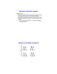
Now we need to pick an ξ that minimizes this. I usually plot it in matlab,<br />
mathematica, maple, or scilab. We can see from the espression that the function is<br />
basically linear in ξ so we suspect that the answer will be either 1/6 or 1/8. For the<br />
ρ = |ψ〉 〈ψ|, η = 1/6, so I would guess the minimum would occur for η = 1/8. This<br />
is true as shown below<br />
The min T r[|ψ〉 〈ψ| ρ] = 0.204<br />
B2.<br />
10
0.25<br />
B1<br />
0.245<br />
0.24<br />
0.235<br />
min Tr[|ψ>
B2 measurements are not consistent with ρ 2 = |ψ〉 〈ψ|.<br />
We write that<br />
maxminT r[|ψ〉 〈ψ| ρ] = 1 √<br />
2 (3ξ)+1 4 (1−3ξ±2 (7/12 − 2ξ)(5/12 − ξ))+ 1 √<br />
2 √ 2 (±2 (3ξ)(5/12 − ξ))<br />
(94)<br />
Notice that this expression is the same as for B1 without a term 1<br />
2 √ √1<br />
2 2<br />
= 1 4<br />
Therefore the max is B1max-1/4=3/4.<br />
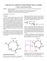
The minimum is negative (≤ −0.46). This is why this measurement of overlap is<br />
not good. The minimum should be zero (for orthogonal states).<br />
We again simply plot with ξ between the bounds of zero and 7/24.<br />
The min trace value is -0.0888<br />
0.25<br />
B2<br />
0.2<br />
0.15<br />
min Tr[|ψ>
maxminT r[|ψ〉 〈ψ| ρ] = 1 2 (2ξ) + 1 1<br />
(3/8 − ξ) +<br />
4 2 √ (2η) (95)<br />
2<br />
Notice how all the terms vanish since |ψ〉 〈ψ| has no overlap with |2〉. Recall that<br />
0 ≤ η ≤ 1/( √ 8) and 3/8 ≥ ξ ≥ 0 We could simply bound the min and max with<br />
these bounds but we have more information.<br />
Using Eq. √88, we need the quadratic problem to have real solutions. After some<br />
algebra this 9/16 − 8η must be real. This means η ≤ 9/(8 · 16) can solve for ξ and<br />
√<br />
find ξ pm = 3/4± 9/16−8η<br />
4<br />
Maximum We choose the maximum ξ for each η and plot the trace. We see that<br />
η = 0 and ξ = 3/8 is the best leading to a trace of 3/8 = 0.375<br />
Minimum We √ set a minimum η=0. Then we need to refer to the other inequality<br />
Eq. 89, 1/4 ≤ 5/4ξ − 2ξ 2 . The smallest value of ξ allowed is ξ = 1/16(5 − √ 17).<br />
We then calculate the minimum Tr is 0.138<br />
3. Bob buys a new detector. It can measure 〈a † a † + aa〉. The values obtained are<br />
B1= √ 3 (ACTUAL HOMEWORK 6/ √ 2 WAS WRITTEN in ERROR THIS VALUE<br />
MEANS THE MEASUREMENT WAS BAD), B2=0, and B3=0. What does this<br />
measure in terms of position and momentum<br />
Update the density matrices.<br />
Calculate the min and max of T r[ρρ] for each case. (One way to measure the<br />
purity. A pure state yields 1 and the most mixed state, 1/3 I, yields 1/3).<br />
Calculate the min and max of T r[|ψ〉 〈ψ| ρ B1 ].<br />
2.3 Solution<br />
Another measurement givesus more insight into the density matrix<br />
We further note<br />
a † a † + aa = ( ˆX 2 /x 0 − ˆP 2 x /P x0 )/2 (96)<br />
and<br />
a † a † + aa = √ 2(|2〉 〈0| + |0〉 〈2|) √ 6(|3〉 〈1| + |1〉 〈3|) (97)<br />
T r[(a † a † + aa)ρ] = 2 √ 2Re(ρ 02 ) + 2 √ 6(|3〉 〈1| + |1〉 〈3|) (98)<br />
13
B1. For B1 this measurement of √ 3 almost tells us the whole density matrix. It<br />
sets ρ 1 13 and as a consequence there is only one value of ξ, ξ = 1/6, that satsifies the<br />
Eq. 37<br />
where<br />
ρ 1 00 = 1/4 (99)<br />
ρ 1 11 = 1/2 (100)<br />
ρ 1 33 = 1/4<br />
√<br />
(101)<br />
ρ 1 01 = ρ 1 10 = 1/8 (102)<br />
ρ 1 03 = ρ 1∗<br />
30 = |ρ 1 13|e −iφ 13<br />
(103)<br />
√<br />
ρ 1 13 = ρ 1 31 = 1/8 (104)<br />
(105)<br />
|ρ 1 03| ≤ 1/4 (106)<br />
ρ 1 could still be a pure state so the max T r[ρ 1 ρ 1 ]=1 and max T r[|ψ〉 〈ψ| |ψ〉 〈ψ|]=1.<br />
For the minimum purity, we set ρ 1 13=0 and find T r[ρ 1 ρ 1 ] = 1−2(1/16) = 7/8. For the<br />
minimum overlap, we set ρ 1 13=-1/4 and find T r[|psi〉 〈psi| ρ 1 ] = 1 − 4(1/16) = 0.75.<br />
B2.<br />
For B2 we have<br />
ρ 2 00 = 7/12 − 2ξ (107)<br />
ρ 2 11 = 3ξ (108)<br />
ρ 2 33 = 5/12 − ξ (109)<br />
ρ 2 01 = ρ 2 10 = 0 (110)<br />
ρ 2 03 = ρ 2∗<br />
30 = |ρ 1 03|e −iφ 03<br />
(111)<br />
ρ 2 13 = −ρ 2∗<br />
31 = ±i|ρ 1 13| (112)<br />
(113)<br />
where<br />
|ρ 2 03| ≤<br />
|ρ 2 13| ≤<br />
√<br />
7/12 − 2ξ<br />
√<br />
3ξ<br />
√<br />
5/12 − ξ (114)<br />
√<br />
5/12 − ξ (115)<br />
7/24 ≥ ξ ≥ 0 (116)<br />
14
We now know the offdiagonal element ρ 2 13 is pure imaginary.<br />
Minimum purity occurs when the offdiagonal elements have minimum value.<br />
Then<br />
T r[ρ 2 ρ 2 ] = (7/12 − 2ξ) 2 + (3ξ) 2 + (5/12 − ξ) 2 (117)<br />
= 74/144 − 3/2ξ + 14ξ 2 (118)<br />
First, we check where the minimum of the quadratic function is. We find that<br />
ξ min = 3/56. This is within the allowed bounds.<br />
minT r[ρ 2 ρ 2 ] = 0.4737 (119)<br />
For the maximum, we use a pure state that agrees with ξ = 0, |Ψ〉 = √ 7<br />
√ |0〉 + 12<br />
5<br />
|3〉. The T r[|Ψ〉 〈Ψ| |Ψ〉 〈Ψ|] = 1.<br />
12<br />
(We said that 1’s were measured out of B2 so this answer is technically wrong.<br />
However, since we didn’t mention the frequency of 1 we can assume that it was<br />
measured only once out of our millions of measurements. The correct answer is<br />
ρ 2 = (1 − ɛ) |Ψ〉 〈Ψ| + ɛ |1〉 〈1|. The max Tr measureing purity is then 1 − ɛ + ɛ 2 ).<br />
B3.<br />
We can then write that<br />
ρ 3 00 = 3/8 − ξ ρ 3 11 = 2ξ (120)<br />
ρ 3 22 = 5/8 − ξ (121)<br />
ρ 3 01 = ρ 3 10 = η (122)<br />
√<br />
ρ 3 12 = ρ 3 12 = ( 1/8 − η)/ √ 2 (123)<br />
ρ 3 20 = −ρ 3 20 = ±i|ρ 3 20| (124)<br />
√<br />
where 1/8 ≥ η ≥ 0.<br />
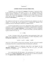
The maximum purity we find numerically to be 0.74. The minimal purity we find<br />
numerically to be 0.45.<br />
Here’s a plot of the max purity. The boundaries defined by the inequalities are<br />
denoted by the sudden jump in color.<br />
15
B3 purity<br />
0.05<br />
0.7<br />
0.1<br />
0.65<br />
ξ<br />
0.15<br />
0.2<br />
0.6<br />
0.25<br />
0.55<br />
0.3<br />
0.5<br />
0.35<br />
0.05 0.1 0.15 0.2 0.25 0.3 0.35<br />
η<br />
0.45<br />
3 Single Molecule NMR<br />
In Problem 1, we assumed a single proton spin NMR Device. Here we look at whether<br />
or not that is possible. We assume in this problem that the H-NMR resonance is at<br />
500 MHz.<br />
1. A magnetic dipole produces a magnetic field B ⃗ = µ 0 ⃗µ<br />
. In QM, we replace<br />
4π r 3<br />
⃗µ with 〈ˆ⃗µ〉. In NMR, 〈ˆµ(t)〉 oscillates in time creating a sinusoidal signal. As a toy<br />
model, assume that the pickup coil transforms the magnetic field into a current by<br />
the following equation I(t) = 2π(1mm)<br />
µ 0<br />
B(t). This current passes through a 1 Ohm<br />
resistor and the voltage drop over the resistor is measured. We will say that NMR is<br />
possible in this toy model when the voltage drop is larger than the thermal voltage<br />
due to Johnson noise.<br />
a. Assume that the spin is at T=0 K. (The resistor is still at 300 K). What<br />
distance r does the pickup coil need to be for NMR to be possible<br />
b. Assume that the spin is at T=300 K. How close does the pickup coil need to<br />
be now<br />
16
3.1 Solution<br />
First calculate the Johsnon Noise, V therm = 4Rk b T ∆f. For our case ∆f = 500MHz,<br />
yielding V therm = 2.9µV.<br />
Now we calculate the V = IR.<br />
V = IR (125)<br />
= 1Ohm 〈µ〉(1mm)<br />
2r 3 (126)<br />
= 1Ohm γ H(1mm)<br />
〈σ<br />
4r 3 Z 〉 (127)<br />
= 1Ohm γ H(1mm)<br />
T r[σ<br />
4r 3 z ρ(T )] (128)<br />
where ρ(T ) is the thermal density matrix at temperature T and γ H = 5.6 Nuclear<br />
Bohr Magnetons = 5.6 × 5.5 × 10 −26 J/T . We need to find r such that V = V therm<br />
We now examine ρ(T ) at two temperatures. At 0 K, the thermal density matrix<br />
is always the ground state. (Proton spin points along the magnetic field).<br />
Consequently,T r[σ z ρ(T )] = 1. We can then calculate the distance to be r = 29<br />
nm. This is already difficult.<br />
For part b we look at the spin at temperatute T =300K. As we discussed in class<br />
this results in a very small magnetic moment. T r[σ z ρ(T )] = 4x10 −5 . This leads to a<br />
distance of r = 1.1nm.<br />
Single spin measurements of electrons involving nm leads and devices at 4K has<br />
been shown. A single spin measurement of a nuclei has been performed in atoms<br />
using the hyperfine interaction to couple the nuclear magnetic dipole to the electron<br />
magnetic dipole and then using the fine structure to couple the electron magnetic<br />
dipole to the electric dipole of the atom.<br />
2. Single molecule fluorescence experiments at room temperature are possible.<br />
Why is this the case (qualitative and/or quantitative argument). Hint: These<br />
experiments involve visible light and an electron dipole.<br />
3.2 Solution<br />
Single molecule NMR is hard at room temperature because the magnetic dipole of<br />
proton is small and the residual or effective magnetic dipole at room temperature is<br />
tiny.<br />
Electric dipole of a molecule is much larger than the magnetic dipole of a nucleus<br />
and, therefore, generates a larger electro-magnetic field when oscillating. See the<br />
17
notes about EM waves. Equally valid are arguments about photon detectors at<br />
visible wavelength but not at 500 MHz.<br />
Since the transition is visible the energy spacing between the levels is large (h<br />
time a few 100 THz). At room temperature most of the population is still in the<br />
electronic ground state. Unlike the case of a nuclear spin, the expectation value for<br />
the dipole element is approximately the same as what it would be at 0 K.<br />
18